Oscillations and Random Perturbations of a FitzHugh-Nagumo System

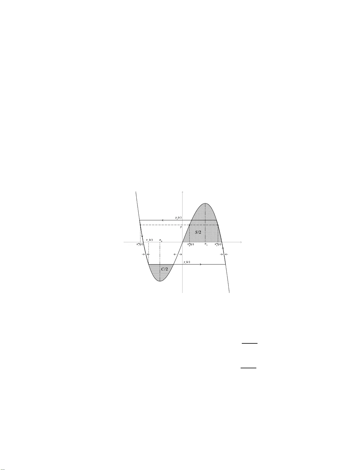
Oscillations and Random P erturbations of a FitzHugh-Nagumo System Cather ine Doss ∗ Mic h` ele Thieull en † No vem b er 2 , 2018 Abstract W e consider a sto chastic p erturb ation of a FitzHugh-Nag u mo system. W e sho w that it is p ossible to generate oscillations for v alues of pa- rameters whic h do not allo w oscillatio n s for the deterministic system. W e also study the ap p earance of a new equilibrium p oint and new bifurcation p arameters du e to the noisy comp onent. Keyw ords: FitzHugh-Nagumo system, fast-slo w system, excitabilit y , equi- librium p oints , bifurcation par a meter, limit cycle , bistable system, random p erturbation, large deviations, metastabilit y , sto c hastic resonance ∗ Lab oratoir e Jacques-L o uis Lions, Bo ˆ ıte 189, Universit ´ e Pierre e t Mar ie Cur ie - Paris 6, 4, Place Jussieu, 75 252 Paris cedex 05, F rance; doss@a nn.jussie u.fr † Lab oratoir e de Probabilit´ es et Mo d` eles Al´ eatoires, Bo ˆ ıte 188, Universit ´ e Pier re et Marie Curie-Paris 6, 4, Plac e Jussieu, , 752 52 P a ris cedex 0 5 , F rance; mich e le.thieullen@upmc.fr 1 1 In tro duction. Let us consider the fo llowing family of deterministic syste ms indexed b y the parameters a ∈ R and δ > 0. δ ˙ x t = − y t + f ( x t ) , X 0 = x (1.1) ˙ y t = x t − a, Y 0 = y (1.2) and their sto c hastic p erturbation by a one dimensional Wiener pro cess ( W t ) as fo llo ws δ dX t = ( − Y t + f ( X t )) dt + √ ǫdW t , X 0 = x (1.3) d Y t = ( X t − a ) dt, Y 0 = y (1.4) The f unction f is a cubic p olynomial: f ( x ) = − x ( x − α )( x − β ) with α < 0 < β . The parameter δ is small. The deterministic system (1.1)-(1.2) is an example of a slo w-fast system: the tw o v ariables x, y ha ve differen t time scales, x t ev olv es ra pidly while y t ev olv es slowly . This system is one v ersion of the so called FitzHugh-Nagumo system and pla ys an imp ortant role in neuronal mo delling. In this con t ext x t denotes the voltage or a c- tion p oten tial of the mem brane o f a single neuron. It w as first pro p osed by FitzHugh and Nag umo (cf. [3], [13 ]). One in terest o f this mo del is that it repro duces p erio dic oscillations observ ed exp erimen tally . Indeed FitzHugh- Nagumo system finds its o r ig in in the nonlinear oscillator mo del pro p osed b y v an der P ol. It is also a simplification of the Ho dgkin-Huxley mo del whic h describes the coupled ev olution of the mem brane p oten tial and the differen t ionic curren ts: existence of differen t time scales enable to pass from a four dimensional mo del to a t wo dimensional o ne. Oscillations can tak e place b e- cause the deterministic system (1.1 )-(1.2) exhibits bifurcations; mor e details will b e giv en in section 3 . Let us men tion that oscillations in this system (1.1)-(1.2) can only o ccur when a ∈ ] a 0 , a 1 [ where a 0 < a 1 are tw o particular v alues of para meter a namely the bifur catio n pa r ameters. Our main in terest in the presen t pap er is to generate oscillations ev en for a < a 0 (symmetrically a > a 1 ) )b y adding a sto c hastic p erturbat io n to the deterministic system. What may b e interpreted as some resonance ty p e effect (cf. [9], [8]). W e will therefore inv estigate p ossible oscillations for system (1.3)-(1.4). The presence of parameter ǫ in tro duces a third scale in the system and the r elativ e strength of δ and ǫ measured b y the ratio ǫ | log δ | δ will determine its ev olution. Our study w as inspired by reference [6] where 2 M. F reidlin considers a random p erturbation of the second o rder equation δ d 2 y t dt 2 = g ( dy t dt , y t ) and p erforms the study of its solution using the theory of large deviations (cf. [5]). See a lso [7] for the study of a more general situa- tion. In our case g ( ˙ y, y ) = y − f ( ˙ y + a ). Although our argumen t is close to M. F re idlin’s, the presence of parameter a leads to a ric her b eha viour. W e prov e the existence of equilibrium p oin t and limit cycle s different fro m t he deterministic ones; as in [6], as w ell as a new bifurcation p o in t whic h did not exist for the deterministic system. Our study relies o n transitions b et w een basins of attra ctio n of stable equilibrium p oin ts due t o noise. Relying on some estimation of a family of exit times(propositions 3 .3 and 3.4) w e study conditions o n the parameters under whic h a con v enient sto c hastic dynamic system approach its main state(prop osition 3.5 ),(whic h corresp onds to the equilibrium p oin t exhibited in main theorem 2.2), or approac h a metastable state (whic h corresp o nds to the limit cycle and t o the new bifurcation pa- rameters exhibited in main theorem 2.1). A g eneral study of slo w-fa st systems p erturbed by noise can b e found in [1]. Bursting oscillations in whic h a sys tem alternates p erio dically b et we en phases of quiescence and phases of rep etitiv e spiking has b een studied for sto c hastically p erturb ed systems in [10] and may b e studied lat er in our sto c hastic setting. W e recall that in the deterministic one a bursting-type b eha viour has b een generated in [2]. The pap er is organized as follo ws. In section 2 we recall basic facts a b out (1.1)-(1.2) and w e state the t wo main theorems (2 .1) and (2.2). Section 3 is dev oted to the application of la rge deviation theory to (1.3)-(1 .4) a nd section 4 to the pro o f of the main theorems. 2 Some Basic Results . 2.1 Deterministic FitzHugh-Nagumo System. In (1.1)-(1.2) let us consider α < 0 < β and f ( x ) = − x ( x − α )( x − β ). In order to in v estigate t he a symptotic b eha viour of ( x t , y t ) one first lo oks for equilibrium p oin ts of the syste m and their stabilit y . The equilibrium p oin ts are define d as t he p oints ( x, y ) where the righ t-hand sides of b ot h equations of the system v anish. F or any v alue of a there is therefore a unique equilibrium p oin t for (1.1)-(1 .2) whic h is ( a, f ( a )). Moreov er let a 0 , a 1 , a 0 < a 1 b e the t w o p oints where f ′ v anishes . The stabilit y of the equilibrium p oint ( a, f ( a )) 3 c hanges when a passes thro ugh the v alue a 0 (resp. a 1 ); a 0 and a 1 are called the bifurcation pa r ameters of the system . Let us fo cus on a 0 ; an analogous argumen t holds for a 1 . By linearizing system (1.1) at ( a 0 + η , f ( a 0 + η )) for η small, w e obtain system ˙ Z = AZ with A = f ′ ( a 0 + η ) δ − 1 δ 1 0 ! A a dmits the t wo eigenv alues λ ± = 1 2 δ ( f ′ ( a 0 + η ) ± i q 4 δ − f ′ 2 ( a 0 + η )). The sign of f ′ ( a 0 + η ) is the same as that of η since f ′ is increasing in the neigh b ourho o d of a 0 . The p o in t ( a 0 + η , f ( a 0 + η )) is therefore an attracting (resp. repulsiv e) f o cus when η < 0 (resp. η > 0). In particular, ( a, f ( a )) is stable when a < a 0 , unstable when a > a 0 . F or a ∈ ] a 0 , a 1 [ the system admits a limit cycle. The bifurcatio n is of Hopf t yp e [4 ] It can b e v erified n umerically that if δ < 0 . 01 the limit cycle is v ery close to the lo op made up with the t wo attracting branc hes o f the curve y = f ( x ) where x 7→ f ( x ) is decreasing and y ∈ [ f ( a 0 ) , f ( a 1 )], and the p ort io ns of the t w o horizon tal segmen ts y = f ( a 0 ), y = f ( a 1 ) connec ting them. When δ → 0 the p erio d of this limit cycle is 0(1); b y example f o r f ( x ) = x (4 − x 2 ) it is equal to 2 ( cf. [14]). 2.2 Main Theorems Consider ( X t , Y t ) the solution of (1.3)-(1 .4 ) and S > 0 giv en in definition 3.3. Let us assume that ǫ > 0 and δ > 0 go to zero in suc h a w ay that for some constan t c > 0. ǫ | log δ | δ → c (2.1) Let us denote by lim ∗ an y limit on ǫ and δ g o ing to 0 under condition (2.1). Theorem 2.1 L et c ∈ ]0 , S [ ; then: 1.If a ∈ ] x − ( c ) , x + ( c )[ wher e x − ( c ) and x + ( c ) ar e intr o duc e d in definition 3 .4; then ther e exist two p erio dic function s Φ a c and Ψ a c given in defin ition 4.2, s.t for al l A , h > 0 , y ∈ ] f ( a 0 ) , f ( a 1 )[ , lim ∗ P ( x,y ) ( Z A 0 | X t − Φ a c ( t ) | 2 dt > h ) = 0 (2.2) lim ∗ P ( x,y ) (sup [0 ,A ] | Y t − Ψ a c ( t ) | > h ) = 0 (2.3) 4 2. If a < x − ( c ) or a > x + ( c ) then for al l y ∈ ] f ( a 0 ) , f ( a 1 )[ , for a l l h > 0 ther e exists ˆ t ( y , h ) such that for al l A > ˆ t ( y , h ) , lim ∗ P ( x,y ) ( sup [ ˆ t ( y ) ,A ] | X t − a | + | Y t − f ( a ) | > h ) = 0 (2.4) Figure 1: Limit cycle when f ( x ) = x (4 − x 2 ) and ǫ | log δ | δ → c Remark In the first case the solution stabilizes when δ → 0 a nd ǫ | log δ | δ → c around a limit cycle defined by c and differen t f rom the one o bt a ined in the deter- ministic case when δ → 0 a nd ǫ = 0 (see figure 1). Moreov er x − ( c ) and b y symmetry x + ( c ) pla y the role o f bifurcation pa rameters for the sto c hastic 5 FitzHugh-Nagumo system (1.3)-(1.4). Indeed for a in the neighborho o d of x − ( c ) but smaller the limit of ( X t , Y t ) is a unique equilibrium p oint, whereas for a in the neigh b orho o d of x − ( c ) but greater it is the graph of a p eriodic function. These bifurcation pa rameters are diff erent from those of the de- terministic syste m (1.1). This theorem is a new resu lt w.r.t. [6]. It is made p ossible b y t he freedom on parameter a . The new limit cycle (Φ a c ( t ) , Ψ a c ( t )) is defined in the same w ay as in [6] Theorem 1 P art 3., provide d w e tak e into accoun t the presence of a in our sys tem. Other regimes are considered in the work of Berglund and Gentz (cf. [1] and references therein). Theorem 2.2 L et c > S . Consi d er x ∗ − ( y ∗ ) and x ∗ + ( y ∗ ) define d in pr op osi- tion 3.2 and definition 3.3; then for al l y ∈ ] f ( a 0 ) , f ( a 1 )[ and for al l h > 0 ther e exists ˆ t ( y , h ) such that for al l A > ˆ t ( y , h ) , 1. If a ∈ ] x ∗ − ( y ∗ ) , x ∗ + ( y ∗ )[ lim ∗ P ( x,y ) ( sup [ ˆ t ( y ) ,A ] | Y t − y ∗ | > h ) = 0 (2.5) 2. If a < x ∗ − ( y ∗ ) or a > x ∗ + ( y ∗ ) , lim ∗ P ( x,y ) ( sup [ ˆ t ( y ) ,A ] ( | X t − a | + | Y t − f ( a ) | ) > h ) = 0 (2.6) Remark : Case 1 ma y b e considered as a degenerate ve r sion of the limit cycle of case 1 theorem 2.1 . In f act y ∗ is a fixed p oint but X t oscillates b et we en x ∗ − ( y ∗ ) and x ∗ + ( y ∗ ). 3 Exit Time, Main State and Metastable State 3.1 Basic results on Large Deviations T h eory Because o f the slo w-fast prop ert y o f FitzHugh-Nagumo systems, the slow v ariable Y t of system (1.3)-(1 .4) may b e in a first appro ximation frozen at the v alue y whic h leads us to the study o f the family of o ne dimensional 6 dynamical systems indexed b y parameter y ,whic h play s a basic role in the study o f FitzHugh-Nag umo systems (1.1)-(1.2) and (1.3)-(1.4): dx y t = ( − y + f ( x y t )) dt, x y 0 = x (3.1) So w e are led to conside r the real v alued deterministic system dx t = b ( x t ) dt, x 0 = x (3.2) and its perturba tion b y a bro wnian motion d ˜ x t = b ( ˜ x t ) dt + √ ˜ ǫdW t , ˜ x 0 = x (3.3) Let us briefly recall some results from [5]. The pro ces s ( ˜ x t ) describ es the mo v ement of a particle on the real line submitted to the force field b ( x ) and to a stationnary Gaussian noise of amplitude √ ˜ ǫ . When ˜ ǫ → 0, ( ˜ x t ) con v erges to the solution ( x t ) of (3.2): ∀ η > 0 ∀ T > 0 lim ˜ ǫ → 0 P (sup [0 ,T ] | ˜ x t − x t | > η ) = 0 (3.4) Ho w eve r b ecause of diffusion due to the presence of noise, some tra jectories of the pro cess ( ˜ x t ) may presen t large deviations from those of the deterministic system ( x t ). Such deviations are measured by means of t he a ctio n functional S T 2 T 1 ( ϕ ) independan t of ˜ ǫ a nd defined b y S T 2 T 1 ( ϕ ) = 1 2 Z T 2 T 1 | ˙ ϕ u − b ( ϕ u ) | 2 du (3 .5 ) when ϕ is absolutely con tin uo us, b y S T 2 T 1 ( ϕ ) = + ∞ otherwise Theorem 3.1 ( [5], L emma 2.1, Chap. 4) L et η > 0 . Then P x (sup [0 ,T ] | ˜ x t − x t | ≥ η ) ≤ exp( − 1 ˜ ǫ [inf ∆ S T 0 ( ϕ ) + o ( 1)]) (3.6) when ˜ ǫ → 0 and wher e ∆ := { ϕ ; ϕ 0 = x, sup [0 ,T ] | ϕ t − x t | ≥ η } . Large deviations theory also provides estimates on the first exit time of ( ˜ x t ) from a domain (cf. [5], Theorem 4.2, Chap. 4). D omains of interes t are basins of attraction of stable equilibrium p oin ts of (3.2). The k ey to ols ar e quasip oten tials. 7 Definition 3.1 Th e quasi p otential of the deterministic system (3.2) w. r. t. a p oint x (also c al l e d tr ansition r ate) is define d as the function u 7→ V ( u ) := inf { S T 2 T 1 ( ϕ ); 0 ≤ T 1 < T 2 , ϕ ( T 1 ) = x, ϕ ( T 2 ) = u } (3.7) Prop osition 3.1 The quasi p otential o f (3.2) w.r.t. x c oincide s with the function u 7→ V ( u ) = − 2 Z u x b ( r ) dr (3.8) Remark : The ab o v e statemen t holds since (3.2) is one dimensional. It also holds in the multidime nsional case when the drift b of (3.2) is a gradien t. Theorem 3.2 L et x ∗ b e a stable e quilibrium p oint of (3.2) such that b ( r ) < 0 for al l r > x ∗ , and b ( r ) > 0 for al l r < x ∗ . L et D b e the b asin of attr action of x ∗ and ˜ τ den ote the fi rs t exit time of ˜ x fr om D . L e t us assume that D =] α 1 , α 2 [ with V ( α 1 ) < V ( α 2 ) . Then for al l x ∈ D and h > 0 , lim ˜ ǫ → 0 P x ( ˜ x ˜ τ = α 1 ) = 1 (3.9) lim ˜ ǫ → 0 P x (e V ( α 1 ) − h ˜ ǫ < ˜ τ < e V ( α 1 )+ h ˜ ǫ ) = 1 (3.10) Remark : With the not ations of Theorem 3.2, with great probability when ˜ ǫ → 0 , the b eha viour o f the pro cess ( ˜ x t ) on a n in terv al [0 , T (˜ ǫ )], in particular whether the pro cess has jump ed out of the basin of attraction D or not, dep ends on the v alue of ˜ ǫ log T ( ˜ ǫ ) compared to V ( α 1 ). 3.2 Tw o F ami lies of Qu asip oten tials. Let us now apply t hese results to the fo llo wing family of one dimensional dynamical systems indexed b y pa r ameter y intro duced in the preceeding subsection. dx y t = ( − y + f ( x y t )) dt, x y 0 = x (3.11) Prop osition 3.2 L et y ∈ ] f ( a 0 ) , f ( a 1 )[ with a 0 and a 1 the two p oints wher e f ′ vanishes. (i) The set { x ∈ R ; f ( x ) = y } c onsists of thr e e p oints x ∗ − ( y ) < x ∗ 0 ( y ) < x ∗ + ( y ) (the e quilibrium p oints of (3.11)) e ach b eing a c ontinuous function of y with b ounde d fi rst and se c ond derivatives. (ii) The two p oints x ∗ ± ( y ) ar e stable. x ∗ 0 ( y ) is unstable . 8 Pro of of Prop osition 3.2 : Left to the reader; w e refer to figure 1-section 2 Definition 3.2 L et us define the two functions V ± on ] f ( a 0 ) , f ( a 1 )[ as fol- lows: V ± ( y ) = − 2 Z x ∗ 0 ( y ) x ∗ ± ( y ) ( − y + f ( u )) du . (3.12) F rom Prop osition 3.1 w e see that V ± ( y ) is the v alue at x ∗ 0 ( y ) of the quasip o- ten tial of (3.2) w.r.t. x ∗ ± ( y ). Both functions V ± ( y ) are strictly monoto ne: V − is strictly increasing, V + is strictly decreasing. Therefore their gr a phs restricted t o ] f ( a 0 ) , f ( a 1 )[ in tersect at a unique p oin t. Definition 3.3 We d enote by ( y ∗ , S ) the interse ction p oin t of the gr aphs of V − and V + . L et E 1 := { y > y ∗ } and E 2 := { y < y ∗ } . Definition 3.4 F or c ∈ ]0 , S [ we denote by y ± ( c ) the p oints of ] f ( a 0 ) , f ( a 1 )[ which satisfy y − ( c ) < y ∗ < y + ( c ) and V − ( y − ( c )) = c = V + ( y + ( c )) . L et us also define x − ( c ) := x ∗ − ( y − ( c )) and x + ( c ) := x ∗ + ( y + ( c )) (cf. figur e 1). Remark : By definition V − ( y ∗ ) = V + ( y ∗ ) = S . F or f ( x ) = 4 x − x 3 , y ∗ = 0 and S = 4. F or an y function U satisfying y − f ( u ) ≡ − ∂ x U / 2 the follo wing iden tities hold: V − ( y ) = U ( x ∗ 0 ( y )) − U ( x ∗ − ( y )) , V + ( y ) = U ( x ∗ 0 ( y )) − U ( x ∗ + ( y )) (3.13) In o ur case suc h a function U is a p olynomial of degree 4 whic h admits x ∗ 0 ( y ) as relativ e maximu m and x ∗ ± ( y ) as relativ e minima. The graph of t he function U ha s tw o w ells with resp ectiv e b ottoms at x ∗ ± ( y ) and one top at x ∗ 0 ( y ). Iden tities (3.1 3 ) express that V ± ( y ) are the respectiv e depths of these w ells. Therefore, on E 1 the we ll with b ottom x ∗ − ( y ) is the deep est one while it is the con tra ry on E 2 . Second, the p ortion of the curv e z = f ( x ) connecting ( x ∗ − ( y ) , y ) to ( x ∗ 0 ( y ) , y ) is situated b elow the horizon t a l line L y := { ( x, z ); z = y } ; th us the p ositiv e quan tity 1 2 V − ( y ) measures the surface of the area limited b y the curv e z = f ( x ) a nd the segmen t of L y on whic h x ∈ [ x ∗ − ( y ) , x ∗ 0 ( y )]. In the same w ay 1 2 V + ( y ) measu r es the surface of the area limited b y t he curv e z = f ( x ) and 9 the segmen t of L y on whic h x ∈ [ x ∗ 0 ( y ) , x ∗ + ( y )] but in this case the p ortion of the curve is abov e the line segmen t. Moreo v er as w e will see in the follow ing section V ± is connected to exit times of diffusions d ˜ Z y t = ( − y + f ( ˜ Z y t )) dt + √ ˜ ǫdW t , ˜ Z y 0 = x (3.14) from the basins of attraction of x ∗ ± ( y ) (cf.Theorem 3.2). 3.3 Exit Times, Main state and Metastable States W e refer the reader to [7] f or the presen t section. Let us recall the fundamen- tal difference b et w een the t w o parameters ǫ and δ . Parameter δ is a lready presen t in the deterministic system (1.1)-(1 .2) where it measures the differ- ence b etw een the time scale of the slow v ariable y t and t he time scale of the fast v ariable x t . In particular a fter the time change s := δ t , the tra jectory ( ˜ x s , ˜ y s ) := ( x δt , y δt ) satisfies ˙ ˜ x s = − ˜ y s + f ( ˜ x s ) (3.15) ˙ ˜ y s = δ ( ˜ x s − a ) (3.16) Since δ is small the comp onen t ˜ y s ma y b e considered as constan t equal to ˜ y 0 . Let us define Z y t to be the family of solutions of δ d Z y t = ( − y + f ( Z y t )) dt + √ ǫdW t , Z y 0 = x. (3.17) W e will also consider the t ime c hange ( ˜ Z y t ) of ( Z y t ) under s := δ t d ˜ Z y s = ( − y + f ( ˜ Z y s )) ds + √ ˜ ǫd ˜ W s , ˜ Z y 0 = x (3.18) with ˜ ǫ = ǫ δ . ( ˜ Z y t ) is the sto c ha stic p erturba t ion of (3.11). In t he tw o following prop ositions w e give crucial estimates on exit time of the resp ectiv e solutio ns of (3.17 ) and (3.18). Prop osition 3.3 L et ˜ τ y 1 (r esp. ˜ τ y 2 ) denote the exit time of ˜ Z y fr om D y 1 (r esp. D y 2 ) which is the b as i n of attr action of x ∗ − ( y ) (r esp. x ∗ + ( y ) ). L e t us r e c al l that D y 1 =] − ∞ , x ∗ 0 ( y )[ (r esp. D y 2 =] x ∗ 0 ( y ) , + ∞ [ ). F r om The or em 3. 2 identity (3.10), for x ∈ D y 1 and h > 0 we obtain ∀ x ∈ ] − ∞ , x ∗ 0 ( y )[ , ∀ h > 0 lim ˜ ǫ → 0 P x (exp( V − ( y ) − h ˜ ǫ ) < ˜ τ y 1 < exp( V − ( y )) + h ˜ ǫ )) = 1 (3.19) 10 A n analo gous r esult holds for x ∈ D y 2 by r eplacing ˜ τ y 1 by ˜ τ y 2 and V − ( y ) by V + ( y ) : ∀ x ∈ ] x ∗ 0 ( y ) , + ∞ [ , ∀ h > 0 : lim ˜ ǫ → 0 P x (exp( V + ( y ) − h ˜ ǫ ) < ˜ τ y 2 < exp( V + ( y )) + h ˜ ǫ )) = 1 (3.20) Prop osition 3.4 L et τ y 1 (r esp. τ y 2 ) denote the first exit time of Z y fr om D y 1 (r esp. D y 2 ). The law of τ y i is the same as the law of δ ˜ τ y i for i = 1 , 2 . L et us assume that ǫ and δ go to 0 in such a way that ǫ δ | log δ | → c ∈ ]0 , + ∞ [ . (3.21) In this c a se we obtain: ∀ x ∈ ] − ∞ , x ∗ 0 ( y )[ , ∀ h > 0 lim P x ( δ c − 1 ( c − V − ( y )+ h ) < τ y 1 < δ c − 1 ( c − V − ( y ) − h ) ) = 1 (3.22) A n analo gous r esult holds for x ∈ D y 2 by r eplacing τ y 1 by τ y 2 and V − ( y ) by V + ( y ) : ∀ x ∈ ] x ∗ 0 ( y ) , + ∞ [ , ∀ h > 0 lim P x ( δ c − 1 ( c − V + ( y )+ h ) < τ y 2 < δ c − 1 ( c − V + ( y ) − h ) ) = 1 (3.23) These tw o prop erties enable us to introduce some remarks ab out t he main theorems stated in the previous section. These remarks are linke d to the notio ns of mainstate and metastable state in tro duced in [5 ]. In a g eneral framew ork ( cf. [7]) the main state is the p o in t to w ar ds which the cost of moving, or the transition rate, is minim um. It is not alwa ys unique: for instance in our bistable case there are tw o main states when y = y ∗ . Before reachin g the main state, the pro ces s ma y reac h metastable ones accessible for shorter time lenghts. Main states ma y b e considered as stable states, whereas metastable states are only stable in some time scale. T o study transitions of (3.18) b et ween the t w o basins of attraction dur- ing [0 , T ( ˜ ǫ )], the relev a n t quan tity to consider is ˜ ǫ log T (˜ ǫ ) whic h w e m ust compare to the transition rates V ± ( y ) given b y (3.12). F or the time scale T ( ˜ ǫ ) = e c ˜ ǫ ; ˜ ǫ log T (˜ ǫ ) = c . So w e m ust compare c to t he transition rates V ± ( y ). Actually this amoun ts to compare first c to S defined in definition 3.3. W e refer again to figure 1. More precisely w e can state using definition 3.3 and 3.4: 11 Prop osition 3.5 ; 1. When c > S the main state of ˜ Z y is e qual to x ∗ + ( y ) (r esp. x ∗ − ( y ) ) if y < y ∗ (r esp. y > y ∗ ). When y = y ∗ the two p oints x ∗ ± ( y ∗ ) ar e b oth main state. 2. When c < S for y ∈ ] y − ( c ) , y + ( c )[ and x ∈ D y 1 (r esp. x ∈ D y 2 ) the metastable state of ˜ Z y is e q ual to x ∗ − ( y ) (r esp. x ∗ + ( y ) ). Pro of of Prop osition 3.5 : Direct consequence of the estimation of the time of exit giv en in prop o sition 3.4. Remark : 1. When c > S the time in terv al [0 , T ( ˜ ǫ )] is long enough so that the pro cess Z y reac hes with great probabilit y a small neigh b orho o d of its main states. And as w e can find an op en in terv al I con taining y ∗ suc h that: ∀ y ∈ I c > max( V − ( y ) , V + ( y )) . (3.24) follo wing pro p osition b oth exit time τ y 1 and τ y 2 tends to 0 in probabilit y so w e can only exp ect results on the slo w comp onen t and the result dep ends on whether the b oundar y b etw een the t w o main states is attra cting o r notas is sho wn in theorem(2.2). 2. On the coun t r a ry when c < S the time in terv a l [0 , T ( ˜ ǫ )] is to o short and the pro cess only reac hes with great probabilit y a neigh b orho o d of a metastable state. In this case we hav e y − ( c ) < y + ( c ) and if w e consider the in terv al ] y − ( c ) , y + ( c )[ when c < V − ( y ) < V + ( y ) and x ∈ D y 1 (resp. c < V − ( y ) < V + − ( y ) and x ∈ D y 2 ), for all y ∈ ] y − ( c ) , y + ( c )[ exit time τ y 1 (resp. τ y 2 )tends to infinit y . So the pr o cess Z y remain in a neighbor ho o d of one metastable state and switc h to the other one as so on as Y t gets o ut of ] y − ( c ) , y + ( c )[; this giv e rise to a limit cyc le as is sho wn in theorem (2.1). 4 Pro of of t he Main Theore ms Definition 4.1 F or a ∈ ] x − ( c ) , x + ( c )[ an d y ∈ ] y − ( c ) , y + ( c )[ as we c an che ck on figur e 1 we have: x ∗ − ( z ) < x − ( c ) < a < x + ( c ) < x ∗ + ( z ) (4.1 ) Then for c ∈ ]0 , S [ , a ∈ ] x − ( c ) , x + ( c )[ and y ∈ ] y − ( c ) , y + ( c )[ , the fo l lowi n g definitions of time dur a tion makes sense T a 1 ( c ) = Z y + ( c ) y − ( c ) dy x ∗ + ( y ) − a and T a 2 ( c ) = Z y + ( c ) y − ( c ) dy | x ∗ − ( y ) − a | (4.2) 12 wher e y ± ( c ) an d x ± ( c ) have b e en in tr o duc e d in Pr op osition 3.2 and Definition 3.4. On the in terv al [0 , T a 1 + T a 2 ]w e can in tro duce the solution of the following ordinary differen tial equations used to define the limit cycle in Theorem Definition 4.2 F or c ∈ ]0 , S [ , a ∈ ] x − ( c ) , x + ( c )[ and y ∈ ] y − ( c ) , y + ( c )[ we define Ψ a c as the c ontinuous p e rio dic function w i th p erio d T a ( c ) = T a 1 ( c ) + T a 2 ( c ) satisfying Ψ a c (0) = y − ( c ) and the o de ˙ Ψ a c ( t ) = x ∗ + (Ψ a c ( t )) − a, t ∈ [0 , T a 1 ( c )[ (4.3) ˙ Ψ a c ( t ) = x ∗ − (Ψ a c ( t )) − a, t ∈ [ T a 1 ( c ) , T a 1 ( c ) + T a 2 ( c )[ (4.4) F or t / ∈ { k T a ( c ) , k T a ( c ) + T a 1 ( c ) , k ∈ Z } , we denote by Φ a c ( t ) the derivative of Ψ a c at t . Existence and regularity of solutions to o des ( 4 .3)-(4.4) follo w from the C 2 regularit y of the functions x ± . . Under the assumptions w e recall that we ha v e (see figure 1) x ∗ − ( z ) < x − ( c ) < a < x + ( c ) < x ∗ + ( z ) (4.5 ) so Ψ a c ( t ) increases from y − ( c ) to y + ( c ) in a durat ion of time equal to T a 1 ( c ) and decreases f rom y + ( c ) to y − ( c ) in a dura tion of time equal to T a 2 ( c ). The p erio dic function Ψ a c is o btained b y contin uously stick ing together at y ± ( c ) the solutions y a ± of the follo wing o des ˙ y a ± ( t ) = x ∗ ± ( y a ± ( t )) − a, y a ± (0) = y (4.6 ) Remark : The function Ψ a c is con tinuous on R differen tiable with con tinuous deriv atives except at p oin ts in the set { k T a ( c ) , k T a ( c ) + T a 1 ( c ) , k ∈ Z } . F or t ∈ [0 , T a 1 ( c )[ the p oint ( x ∗ + (Ψ a c ( t )) , Ψ a c ( t )) b elongs to the right stable branc h; f o r t ∈ [ T a 1 ( c ) , T a 1 ( c ) + T a 2 ( c )[ the p oint ( x ∗ − (Ψ a c ( t )) , Ψ a c ( t )) b elongs to the left stable branch. Pro of of Theorem 4. 1. Case a ∈ ] x − ( c ) , x + ( c )[: a) Let y < y − ( c ) and x ∈ D y 1 . Then lim ∗ P x ( τ y 1 = 0) = 1 since V − ( y ) < V − ( y − ( c )) = c (remem b er that V − is strictly increasing). Therefore the 13 pro cess ( X t ) lea ve s D y 1 instan taneously and is a t t r acted to a neighborho o d of x ∗ + ( y ) > x + ( c ). The p o in t ( X t , Y t ) remains in a neighbourho o d of the branc h v = f ( u ) containing ( x ∗ + ( y ) , y ) and Y t increases as lo ng as X t > x + ( c ) since d Y t = ( X t − a ) dt . Ho we ver iden tit y (3.23) implies that lim ∗ P x ( τ z 2 = + ∞ ) = 1 for z < y + ( c ) (resp. lim ∗ P x ( τ z 2 = 0) = 1 for z > y + ( c ) ). Therefore the p oin t ( X t , Y t ) is instan taneously attracted to a neigh b orho o d of ( x ∗ − ( y + ( c )) , y + ( c )) a fter Y t has crossed y + ( c ) since the sp eed o f Y t is strictly p ositiv e in a neighbourho o d of ( x + ( c ) , y + ( c )). The argumen t is then the same as b efor e. W e detail it for completene ss. Since x ∗ − ( y + ( c )) < x − ( c ) < a , the second co ordinate Y t decreases as long as X t − a < 0. How eve r iden tity (3 .22) implies that lim ∗ P x ( τ z 1 = + ∞ ) = 1 for z > y − ( c ) (r esp. lim ∗ P x ( τ z 1 = 0) = 1 for z < y − ( c )). Therefore the p oint ( X t , Y t ) is instantaneous ly captured b y ( x ∗ + ( y − ( c )) , y − ( c )) after Y t has crossed y − ( c ). Henc e ( X , Y ) con v erges in probabilit y to a limit cycle of p erio d T a ( c ) = T a 1 ( c ) + T a 2 ( c ). b) Let y > y − ( c ) and x ∈ D y 1 . By iden tity 3.22 lim ∗ P x ( τ y 1 = + ∞ ) = 1, the fast pro ces s ( X t ) is attracted to x ∗ − ( y ). After this first phase, o ne can apply the same argumen t as in a). 2.Case a < x − ( c ). As already men tioned in section 3, when c < S , the relev an t states are the metastable ones. The assumption a < x − ( c ) implies f ( a ) > y − ( c ). Let V b e a small neigh b orho o d V of ( a, f ( a )). Let us first assume that V is so small that all ( u , v ) ∈ V satisfies v > y − ( c ) and a c- cordingly u < x − ( c ). Let ( X t , Y t ) start from ( u , v ). In particular u ∈ D v 1 and τ v 1 = + ∞ since V − ( v ) > c . Then ( Y t ) will ev olv e lik e the solution of ˙ v t = x ∗ − ( v t ) − a , v 0 = v for whic h f ( a ) is a stable equilibrium p oin t. Let us no w assume that there are p oin ts ( u , v ) ∈ V such that v < y − ( c ). Then ( X t ) instan taneously jumps to the right stable branc h; ( Y t ) b ecomes close to the solution o f ˙ v t = x ∗ + ( v t ) − a and therefore increases un til it reac hes y + ( c ). A t that time it jumps t o the left stable bra nc h and w e are bac k to the previous argumen t since then ( Y t ) becomes close to the solution of ˙ v t = x ∗ − ( v t ) − a . Let us notice that for the slow v ariable Y t w e get a result using the uniform norm by large deviation estimates but for the quic k v ariable X t the result is form ulated in L 1 norm thanks t o equation (1.4). Pro of of Theorem 2.2. When c > S , as pointed out in subsection (3) Z y has time to r each it s main state so the ev olution o f Y t is close to the solution of ˙ v t = x ∗ + ( v t ) − a pro vided v t < y ∗ 14 ˙ v t = x ∗ − ( v t ) − a pro vided v t > y ∗ and it dep ends on whether the b oundary { y ∗ } b et wee n E 1 := { y > y ∗ } and E 2 := { y < y ∗ } is attractive for this system or not(cf. [7]). If a ∈ ] x ∗ − ( y ∗ ) , x ∗ + ( y ∗ )[ the b oundary is attractiv e. This is not the case when a < x ∗ + ( y ∗ nor whe n a > x ∗ + ( y ∗ ). 1. Let x ∗ − ( y ) < a < x ∗ + ( y ∗ ). The p oint y ∗ is an attracting b oundary since x ∗ − ( y ∗ ) − a < 0 < x ∗ + ( y ∗ ) − a . Assume for example that Y 0 = y < y ∗ that is y ∈ E 2 . The ev olution of ( Y t ) is close to the solution of ˙ Y t = x ∗ + ( Y t ) − a . Therefore since x ∗ + ( y ) > a , pro cess ( Y t ) starts increasing un til it reac hes y ∗ . After it has reac hed y ∗ , the ev olution of ( Y t ) is close to the solution of Y 0 = y ∗ , ˙ Y t = B ( Y t ) where B is a v ector field ta ngen t to b oundary (cf. [7] Theorem 1) whic h is the 0-dimensional manifold { y ∗ } ; therefore B is zero and Y t ≡ y ∗ . The time ˆ t ( y , h ) is the time necessary t o reac h a small ball B ( y ∗ , h ). If y ∈ E 1 the ev olution of ( Y t ) is close to the solution of ˙ Y t = x ∗ − ( Y t ) − a . In this case pro cess ( Y t ) starts decreasing since x ∗ − ( y ) < a until it reac hes y ∗ . The argument and the conclusion are then iden tical to the preceeding case. 2. Let a > x ∗ + ( y ). The p oin t y ∗ is no t an attracting b oundary since x ∗ − ( y ∗ ) − a = < 0 and x ∗ + ( y ∗ ) − a < 0. Let us assume for example that Y 0 = y ∈ E 2 . The ev olution of ( Y t ) is close to the solution of ˙ Y t = x ∗ + ( Y t ) − a . The v a lue f ( a ) is a stable equilibrium for ( Y t ). If x ∗ + ( y ) > a , pr o cess ( Y t ) starts increasing un t il it reache s f ( a ) to whic h it is at t racted. If now x ∗ + ( y ) < a the arg umen t and the conclusion are the same except that ( Y t ) starts decreasing. If y ∈ E 1 the evolution of ( Y t ) is close to the solution o f ˙ Y t = x ∗ − ( Y t ) − a . Since x ∗ − ( y ∗ ) − a < 0 pro ces s( Y t ) starts decreasing un til it crosses y ∗ (whic h is not attractive ) to wards E 2 . Then w e are bac k to the previous case . 3. The case a < x ∗ − ( y ) is treated analogously . Ac knowledgm ent. W e thank Prof. Mark F reidlin for sending us a copy of his pap er [7] which w as not a v ailable to us. 15 References [1] Berglund, N., G en tz, B., Noise-Ind uc e d Phe nomena in S l o w-F ast Dy- namic al Systems: A Sample Paths Appr o a ch. Springer (2006) [2] Do ss, C., F ran¸ coise, J.-P ., Piquet, C., it Bursting oscillations in tw o coupled Fitzh ug h-Nagumo sys t em. ComplexUs, v ol.2, p 1-1 1 (2003) [3] FitzHugh, R., Impulses and physiolo gic al states in the or etic al mo dels of nerve membr ane. Biophys . J., 445-466 (1961 ) [4] F ra n¸ coise, J.- P . Oscil lations en biolo g i e . Analyse qualitative et mo d` eles. Collection Math´ ematiques et Applications V ol. 46, SMAI Springer 20 0 5 [5] F reidlin, M.,I., W en tzell, A., D., R andom p erturb a tion of dynamic al sys- tems. Springer NY (198 4) [6] F reidlin, M., I., On stable oscil lations and Equilibrium Induc e d by Smal l Noise. , J. of Stat. Ph ys., V ol. 103, Nos. 1/2, 283-3 00 (20 01) [7] F reidlin, M., I., On s to chastic p erturb ation of dynamic al systems with fast and slow c om p onen ts. , Sto c hastics and Dynamics, V ol. 1, N. 2 , 261- 281 (2001) [8] Gammaito ni, L., Ha nggi, P ., Jung, P ., Marches oni, F., Sto chastic R eso- nanc e . Rev. of Modern Ph ysics 70 (1 ) 223- 287 (1998) [9] Herrmann, S., Imk eller, P ., The exit pr oblem for diffusion with time p erio dic drif t and sto c hastic r esonanc e. , Annals of Applied Probability 15 (1A) 39-68 ( 2 001) [10] Hitczenk o, P ., Medv edev , G.S. Bursting O scil lations induc e d by smal l noise. Preprint arXiv:071 2 .4074v1 [nlin.A O] 25 Dec 200 7 [11] Keener, Sneyd, Mathematic al Physiolo gy. Mathematical Biology . Inter- disciplinary Applied Mathematics, Springer (1 998) [12] Murray , J., D., Mathematical Biology . V o l. 1 a nd 2 , 2nd edition. Springer (2002) [13] Nagumo, J., S., Arimoto, S., Y oshizaw a, S., An active pulse tr ansm ission line simulating nerve axon. Pro c. IRE, 50, 20 6 1-2071 (1962 ) 16 [14] Piquet, C., P ersonnal comm unication. 17