Applied Categories and Functors for Undergraduates

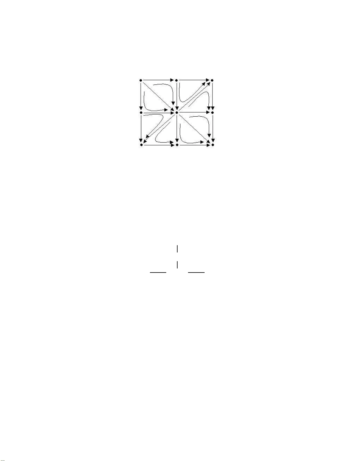
Applied Categories and F unctors for Undergraduates Vladimir G. Iv ancevic ∗ Tijana T. Iv ancevic † Abstract These are lecture notes for a 1–s emester undergraduate course (in computer science, mathematics, ph ysics, engineer ing, chemistry or biology) in applied categorical meta- language. The only necessa ry background for comprehensive r e ading o f these notes are first-year calculus and linea r alge br a. Con ten ts 1 In tro duction 2 2 Sets and Maps 2 2.1 Notes from Set Theory . . . . . . . . . . . . . . . . . . . . . . . . . . . . . . 2 2.2 Notes F rom Calculus . . . . . . . . . . . . . . . . . . . . . . . . . . . . . . . 3 2.2.1 Maps . . . . . . . . . . . . . . . . . . . . . . . . . . . . . . . . . . . 3 2.2.2 Algebra of Ma ps . . . . . . . . . . . . . . . . . . . . . . . . . . . . . 4 2.2.3 Comp ositions of Maps . . . . . . . . . . . . . . . . . . . . . . . . . . 4 2.2.4 The Chain Rule . . . . . . . . . . . . . . . . . . . . . . . . . . . . . 4 2.2.5 In tegratio n and Change of V ariables . . . . . . . . . . . . . . . . . . 5 2.3 Notes from General T op ology . . . . . . . . . . . . . . . . . . . . . . . . . . 5 2.3.1 T op ological Space . . . . . . . . . . . . . . . . . . . . . . . . . . . . 6 2.3.2 Homotop y . . . . . . . . . . . . . . . . . . . . . . . . . . . . . . . . . 7 2.4 Comm utativ e Diagrams . . . . . . . . . . . . . . . . . . . . . . . . . . . . . 9 3 Categories 10 4 F unctors 14 ∗ Vladimir.Iv ancevic@dsto.defence.gov.au † Tijana.Iv ancevic@alumni.adelaide.edu.au 1 5 Natural T ransformations 17 5.1 Comp ositions of Natural T ransformations . . . . . . . . . . . . . . . . . . . 18 5.2 Dinatural T ransformations . . . . . . . . . . . . . . . . . . . . . . . . . . . . 19 6 Limits and Colimits 20 7 Adjunction 21 7.1 Application: Ph ysiologic al S en sory–Motor Adjunction . . . . . . . . . . . . 22 8 App endix: Groups and Related Algebraic Structures 23 1 In tro duction In mo dern mathematical sciences whenever one defines a new class of mathematical ob- jects, one pr o ceeds almost in the next br eath to sa y what kind s of maps b etw een ob jects will b e considered [1, 2, 3, 4, 5 ]. A general f r amew ork for dealing with situations wh ere w e hav e some obje cts and maps b etwe en obje cts , lik e sets and fu nctions, v ector spaces and linear op erators, p oints i n a space and paths b et w een p oin ts, etc. – giv es the mo dern met- alanguage of ca tegories and functors. Cat egories are mathematical univ erses and fu nctors are ‘pro jectors’ from one univ erse o n to another. 2 Sets and Maps 2.1 Notes from Set Theory Giv en a map (o r, a f u nction) f : A → B , the set A is ca lled t he domain of f , and denoted Dom f . The set B is called the c o domain of f , and denoted Co d f . Th e co domain is not to b e confused with the r ange o f f ( A ), whic h is in general only a subset o f B . A map f : X → Y is called inje ctive , or 1–1, or an inje ction , iff f or ev er y y in the co domain Y there is at most o ne x in the domain X with f ( x ) = y . Put another w a y , giv en x and x ′ in X , if f ( x ) = f ( x ′ ), then it follo ws that x = x ′ . A map f : X → Y is called surje c tive , or onto , or a surje ction , iff for ev ery y in the codomain Cod f ther e is at le ast one x in the domain X with f ( x ) = y . Put another wa y , the r ange f ( X ) is equ al to the co d omain Y . A map is bije ctive iff it is b oth injectiv e and s u rjectiv e. Injectiv e functions are cal led monomor phisms , and surjectiv e fu nctions are c alled epimorph isms in the c ate gory of sets (see b elo w). Bijectiv e fu nctions are c alled isomorphism s . 2 A r elation is any su bset of a Cartesian pr o duct (see b elo w). By defin ition, an e q uiv- alenc e r elation α on a set X is a relat ion whic h is r eflexiv e , symmetric al a nd tr ansitive , i.e., relation that satisfies the follo wing thr ee co nditions: 1. R eflexivity : eac h elemen t x ∈ X is equiv alen t to itself, i.e. , xαx ; 2. Symmetry : for any t w o elemen ts a, b ∈ X , aαb imp lies bαa ; and 3. T r ansitivity : aαb and bαc implies aαc . Similarly , a relation ≤ defines a p artial or der on a set S if it has the follo wing prop erties: 1. R eflexivity : a ≤ a for all a ∈ S ; 2. A ntisymmetry : a ≤ b and b ≤ a implies a = b ; and 3. T r ansitivity : a ≤ b and b ≤ c implies a ≤ c . A p artial ly or der e d set (or p oset ) is a set tak en together with a p artial ord er on it. F orm ally , a partially ordered set is defi n ed as an ord ered pair P = ( X , ≤ ), wh ere X is called the gr ound se t of P and ≤ is the partial order of P . 2.2 Notes F r om Calculus 2.2.1 Maps Recall that a map (or, function ) f is a rule that assigns to eac h elemen t x in a set A exactly one elemen t, c alled f ( x ), in a set B . A map could b e th ough t of as a machine [[ f ]] with x − inp ut (the domain of f is the set of all p ossible inputs) and f ( x ) − outpu t (the r ange of f is the set of al l p ossible outputs) [6] x → [[ f ]] → f ( x ) . There are f ou r p ossible wa ys to represen t a fun ction (or map): (i) ve rbally (by a descrip tion in words); (ii ) numerically (b y a table of v alues); (iii) visually (by a graph); and (iv) algebraical ly (by an explicit form ula). T he most common metho d for visu alizing a fun ction is its gr aph . If f is a fu nction with domain A , then its graph is the set of ord ered input– output pairs { ( x, f ( x )) : x ∈ A } . A generalizati on of the graph concept is a concept of a cr oss–se ction of a fibr e bund le , whic h is one of the co re geometrica l ob j ects for dynamics of complex systems (see [4]). 3 2.2.2 Algebra of Maps Let f and g b e maps w ith domains A and B . Then th e m ap s f + g , f − g , f g , and f /g are defined as follo ws [6] ( f + g )( x ) = f ( x ) + g ( x ) domain = A ∩ B , ( f − g )( x ) = f ( x ) − g ( x ) domain = A ∩ B , ( f g )( x ) = f ( x ) g ( x ) d omain = A ∩ B ,  f g  ( x ) = f ( x ) g ( x ) domain = { x ∈ A ∩ B : g ( x ) 6 = 0 } . 2.2.3 Comp ositions of Maps Giv en tw o maps f and g , the comp osite map f ◦ g , called the c omp osition of f and g , is defined b y ( f ◦ g )( x ) = f ( g ( x )) . The ( f ◦ g ) − machine is composed of the g − mac hine (fir s t) and then t he f − mac hin e [6], x → [[ g ]] → g ( x ) → [[ f ]] → f ( g ( x )) . F or example, sup p ose that y = f ( u ) = √ u and u = g ( x ) = x 2 + 1. Since y is a fun ction of u and u is a fun ction of x , it follo ws that y is ultimate ly a f u nction of x . W e calculate this by sub stitution y = f ( u ) = f ◦ g = f ( g ( x )) = f ( x 2 + 1) = p x 2 + 1 . 2.2.4 The Chain Rule If f and g are b oth differen tiable (or smo oth, i.e., C ∞ ) maps and h = f ◦ g is th e comp osite map defined b y h ( x ) = f ( g ( x )), then h is differen tiable and h ′ is giv en by th e pro du ct [6] h ′ ( x ) = f ′ ( g ( x )) g ′ ( x ) . In Leibniz notatio n, if y = f ( u ) and u = g ( x ) are b oth differen tiable maps, then dy dx = dy du du dx . The reason for the name chain rule b ecomes clear if w e add another link to the c hain. Supp ose that w e ha v e one more differentia ble map x = h ( t ). Then, to calculate the deriv ativ e of y with resp ect to t , we use th e c hain ru le t wice, dy dt = dy du du dx dx dt . 4 2.2.5 Integration and Change of V ariables Giv en a 1–1 con tinuous (i.e ., C 0 ) map F with a nonzero Jac obian    ∂ ( x,. .. ) ∂ ( u,. .. )    that maps a region S on to a region R (see [6]), w e ha ve the foll o win g sub s titution form ulas: 1. F or a single in tegral, Z R f ( x ) dx = Z S f ( x ( u )) ∂ x ∂ u du ; 2. F or a double int egral, Z Z R f ( x, y ) dA = Z Z S f ( x ( u, v ) , y ( u, v ))     ∂ ( x, y ) ∂ ( u, v )     dudv ; 3. F or a triple inte gral, Z Z Z R f ( x, y , z ) dV = Z Z Z S f ( x ( u, v, w ) , y ( u, v , w ) , z ( u, v , w ))     ∂ ( x, y , z ) ∂ ( u, v, w )     dudv dw ; 4. Generalization to n − tuple in tegrals is obvio us. 2.3 Notes from General T op ology T op olo gy is a kind of abstr action of Euclidean geometry , an d also a natural framew ork for the study of c ontinuity . 1 Euclidean geometry is abstr acted by regarding triangles, circles, and squares as b eing the same basic ob ject. Contin uity en ters b ecause in saying this one h as in mind a c ontinuous deformat ion of a triangle in to a square or a circle, or an y arbitrary shap e. O n the other hand, a disk with a hole in the cen ter is top ologically differen t from a circle or a squ are b ecause one cannot create or destro y holes b y con tinuous deformations. T hus using topological metho ds one do es not exp ect to b e able to iden tify a geometrical figure as b eing a triangle or a square. Ho w ev er, on e d o es exp ect to b e able to detect the presence of gross features suc h as holes or the fact that the figure is made up of t w o d isjoin t pieces etc. In this wa y top ology p ro duces theorems that are usu ally qualitativ e in nature – they ma y assert, for example, the existence or non–existence of an ob ject. They will not, in g eneral, giv e the means for its construction [7]. 1 Intuitiv ely speakin g, a function f : R − → R is continuous near a p oint x in its domain if its v alue does not jump th ere. That is, if we just tak e δ x to b e small enough, the tw o function v alues f ( x ) and f ( x + δx ) should approac h eac h other arbitrarily closely . I n more rigorous terms, this leads to the follo wing definition: A function f : R − → R is continuous at x ∈ R if for all ǫ > 0, there exists a δ > 0 such that for all y ∈ R with | y − x | < δ , we hav e th at | f ( y ) − f ( x ) | < ǫ . The whole funct ion is called con tin uous if it is conti nuous at every p oint x . 5 2.3.1 T op ological Space Study of top ology starts with the fundamental notion of top olo gic al sp ac e . Let X b e an y set and Y = { X α } denote a collectio n, finite or infi n ite of su bsets of X . Then X and Y form a top ologica l sp ace pro vid ed the X α and Y satisfy: 1. An y finite or infinite sub colle ction { Z α } ⊂ X α has the prop erty that ∪ Z α ∈ Y ; 2. An y finite sub c ol le ction { Z α 1 , ..., Z α n } ⊂ X α has the prop erty that ∩ Z α i ∈ Y ; and 3. Both X and the empt y set b elong to Y . The set X is then called a top ological sp ace and the X α are called op en sets . The c h oice of Y satisfying (2) is said to giv e a top ology to X. Giv en t w o top ological spaces X and Y , a map f : X → Y is c ontinuous if the inv erse image of an op en set in Y is a n op en set in X . The main general idea in topology is to study sp aces which can b e con tinuously d e- formed into one another, namely the idea of home omorphism . If w e ha v e t wo top ological spaces X and Y , then a map f : X → Y is called a homeomorphism iff 1. f is con tinuous ( C 0 ), and 2. There exists an inv erse of f , denoted f − 1 , whic h is also co n tin u ous. Definition (2) implies that if f is a homeomorph ism then so is f − 1 . Homeomorphism is the main top ologica l example of r eflexive , symmetric al and tr ansitive r elation , i.e. , e quiv alenc e r elation . Homeo morphism divides all top ological spaces u p into e quivalenc e classes . In other words, a pair of top ological spaces, X and Y , b elong to the same equ iv alence class if they are homeomorphic. The second example of top ological equiv alence relation is homotopy . While homeo- morphism generat es equiv alence classes wh ose mem b ers are top ologica l spaces, homoto p y generates equiv alence classes whose m emb ers are con tin u ous ( C 0 ) maps. Consider t w o con tinuous maps f , g : X → Y b et wee n top ological spaces X and Y . Then the map f is said to b e homotopic to the map g if f can be con tin u ously d eformed in to g (see b elo w for the precise definition of homotop y). Homotop y is an equiv alence relation w hic h divides the space of con tin uous maps b etw een t w o top ological spaces in to equiv alence classes [7]. Another imp ortan t notions in top ology are c overing , c omp actness and c onne cte dness . Giv en a family of sets { X α } = X sa y , then X is a c overing of another set Y if ∪ X α con tains Y . If all the X α happ en to b e op en sets th e co v ering is called an op en c overing . No w consider the set Y and all its p ossible op en cov erings. The set Y is c omp act if for every op en co v ering { X α } with ∪ X α ⊃ Y there alw a ys exists a finite su b cov ering { X 1 , ..., X n } of Y with X 1 ∪ ... ∪ X n ⊃ Y . Again, w e define a set Z to b e c onne cte d if it cannot b e 6 written as Z = Z 1 ∪ Z 2 , where Z 1 and Z 2 are b oth op en n on–empt y sets and Z 1 ∩ Z 2 is an empt y set. Let A 1 , A 2 , ..., A n b e closed subspaces of a topological space X su c h that X = ∪ n i =1 A i . Supp ose f i : A i → Y is a fun ction, 1 ≤ i ≤ n , suc h that f i | A i ∩ A j = f j | A i ∩ A j , (1 ≤ i, j ≤ n ) . (1) In this case f is con tin uou s iff eac h f i is. Using this pro cedure we can define a C 0 − function f : X → Y b y cutting up the sp ace X into closed sub s ets A i and definin g f on eac h A i separately in suc h a wa y that f | A i is ob viously cont in uous; we then hav e only to c h ec k that the differen t definitions agree on the overlaps A i ∩ A j . The unive rsal pr op erty of the Cartesian pr o duct : let p X : X × Y → X , and p Y : X × Y → Y b e the pr oje ctions on to the fir st and second factors, resp ectiv ely . Giv en an y pair of fun ctions f : Z → X and g : Z → Y there is a unique fun ction h : Z → X × Y suc h that p X ◦ h = f , and p Y ◦ h = g . F u nction h is con tinuous iff b oth f and g are. This prop erty c haracterizes X × Y up to isomorph ism. In particular, to c hec k that a giv en fun ction h : Z → X is cont in uous it will suffi ce to c hec k that p X ◦ h and p Y ◦ h are con tinuous. The universal pr op erty of the quotient : let α b e an equiv alence relation on a top ological space X , let X/α d enote the sp ac e of e quivalenc e classes and p α : X → X/α the natur al pr oje c tion . Giv en a fun ction f : X → Y , there is a fu nction f ′ : X/α → Y with f ′ ◦ p α = f iff xαx ′ implies f ( x ) = f ( x ′ ), for all x ∈ X . In this case f ′ is con tinuous iff f is. This prop erty c haracterizes X/α up to homeomorphism. 2.3.2 Homotop y No w we return to t he fund amen tal n otion of homotop y . Let I b e a compact u n it i n terv al I = [0 , 1]. A homotopy from X to Y is a contin uous function F : X × I → Y . F or eac h t ∈ I one has F t : X → Y d efined by F t ( x ) = F ( x, t ) f or all x ∈ X . The fu nctions F t are called the ‘sta ges’ of t he homotop y . If f , g : X → Y are tw o con tin u ous maps, w e sa y f is homotopic to g , and wr ite f ≃ g , if there is a homotop y F : X × I → Y suc h that F 0 = f and F 1 = g . In other words, f can b e con tinuously deformed into g thr ou gh the stage s F t . If A ⊂ X is a subspace, then F is a h omotop y relativ e to A if F ( a, t ) = F ( a, 0), for all a ∈ A, t ∈ I . The homotop y relation ≃ is an equiv alence relation. T o pro ve that we ha v e f ≃ f is ob vious; tak e F ( x, t = f ( x ), for all x ∈ X , t ∈ I . If f ≃ g and F is a homotopy from f to g , then G : X × I → Y d efi ned by G ( x, t ) = F ( x, 1 − t ), is a homoto p y from g to f , i.e., g ≃ f . If f ≃ g with h omotop y F and g ≃ f with homotop y G , then f ≃ h with homotop y H d efined b y H ( x, t ) =  F ( x, t ) , 0 ≤ t ≤ 1 / 2 G ( x, 2 t − 1) , 1 / 2 ≤ t ≤ 1 . 7 T o sho w that H is con tinuous w e use the relati on (1). In this wa y , the set of all C 0 − functions f : X → Y b etw een t w o top ological spaces X and Y , called the function sp ac e and denoted b y Y X , is partitioned in to equiv alence classes under th e r elation ≃ . Th e equiv alence classes are called homotopy classes , the homotop y class of f is d enoted b y [ f ], and the set of all h omotop y classes is denoted by [ X ; Y ]. If α is an equiv alence relation on a top olog ical sp ace X and F : X × I → Y is a homotop y such t hat eac h stage F t factors through X/α , i.e. , xαx ′ implies F t ( x ) = F t ( x ′ ), then F in duces a homoto p y F ′ : ( X/α ) × I → Y suc h that F ′ ◦ ( p α × 1) = F . Homotop y theory h as a r an ge of applications of its own, outside top ology and geom- etry , as for example in p ro ving Cauc h y theorem in complex v ariable theory , or in solving nonlinear equations of artificial neural net works. A p ointe d set ( S, s 0 ) is a se t S together with a distinguished p oin t s 0 ∈ S . Similarly , a p ointe d top olo g ic al sp ac e ( X , x 0 ) is a space X together with a d istinguished point x 0 ∈ X . When we are concerned with p ointe d spaces ( X, x 0 ) , ( Y , y 0 ), etc, we alw ays require that all functions f : X → Y shell preserve base p oint s, i.e., f ( x 0 ) = y 0 , and that all homotopies F : X × I → Y b e relativ e to the b ase p oint , i.e., F ( x 0 , t ) = y 0 , for all t ∈ I . W e denote the homotop y classes of base p oint–preserving functions b y [ X, x 0 ; Y , y 0 ] (where homotopies are r elativ e to x 0 ) . [ X , x 0 ; Y , y 0 ] is a p ointe d set with base p oin t f 0 , the c onstan t function: f 0 ( x ) = y 0 , for all x ∈ X . A p ath γ ( t ) from x 0 to x 1 in a top ological s p ace X is a con tinuous map γ : I → X with γ (0) = x 0 and γ (1) = x 1 . Thus X I is the space of all paths in X with the co mpact– op en top ology . W e in tro duce a relation ∼ on X by sa ying x 0 ∼ x 1 iff there is a path γ : I → X from x 0 to x 1 . Clearly , ∼ is an equiv alence r elation; the set of equiv alence classes is d enoted b y π 0 ( X ). Th e elemen ts of π 0 ( X ) are called the p ath c omp onents , or 0 − c omp onents of X . If π 0 ( X ) con tains just one elemen t, then X is cal led p ath c onne cte d , or 0 − c onne cte d . A close d p ath , or lo op in X at the p oint x 0 is a p ath γ ( t ) for wh ic h γ (0) = γ (1) = x 0 . The inverse lo op γ − 1 ( t ) b ased at x 0 ∈ X is defined by γ − 1 ( t ) = γ (1 − t ), for 0 ≤ t ≤ 1 . Th e homotopy of lo ops is the p articular case of the ab ov e defined h omotop y of con tinuous maps. If ( X , x 0 ) is a p oin ted s p ace, then we m a y regard π 0 ( X ) as a p oin ted set with the 0 − comp onent of x 0 as a base p oint. W e use the n otation π 0 ( X, x 0 ) to denote p 0 ( X, x 0 ) though t of as a p ointed set. If f : X → Y is a map then f sends 0 − comp onen ts of X in to 0 − comp onents of Y and h ence d efines a fu nction π 0 ( f ) : π 0 ( X ) → π 0 ( Y ). S imi- larly , a base p oin t–preserving map f : ( X, x 0 ) → ( Y , y 0 ) ind uces a map of p oin ted sets π 0 ( f ) : π 0 ( X, x 0 ) → π 0 ( Y , y 0 ). In this w a y defined π 0 represent s a ‘fu nctor’ f rom the ‘categ ory’ of top ological (p oint ) spaces to the underlying c ategory of (point) sets (see the next subsection). The fundamental g r oup (introdu ced b y Po incar ´ e), denoted π 1 ( X ), of a p oin ted space ( X, x 0 ) is the group (see App end ix) formed b y the equiv alence classes of the set of all 8 lo ops , i.e., closed h omotopies with initial and final p oin ts at a giv en base p oin t x 0 . The iden tit y elemen t of this group is the set of all p aths h omotopic to the degenerate path consisting of the p oint x 0 . 2 The fundamental group π 1 ( X ) o nly dep ends on the homotop y t yp e of the space X , that is, f u ndamenta l groups of homeo morphic spaces are isomorphic. Com binations of top ology and calculus give differen tial top ology and differenti al ge- ometry . 2.4 Comm utative Diagrams The c ate gory the ory (see b elo w) w as b orn with an observ ation that many prop erties of mathematical systems can b e un ified and simplified by a presen tatio n with c ommutative diagr ams of arr ows [1, 2]. Eac h arrow f : X → Y r epresen ts a fu nction (i.e., a map, transformation, op erator); th at is, a source (domain) set X , a targe t (codomain) set Y , and a r ule x 7→ f ( x ) whic h assigns to e ac h elemen t x ∈ X an element f ( x ) ∈ Y . A typical diagram of sets and functions is X Y ✲ f h ❅ ❅ ❅ ❅ ❘ Z ❄ g or X f ( X ) ✲ f h ❅ ❅ ❅ ❅ ❘ g ( f ( X )) ❄ g This diagram is c ommutative iff h = g ◦ f , where g ◦ f is the usu al comp osite function g ◦ f : X → Z , defined b y x 7→ g ( f ( x )). Similar comm utativ e diagrams apply in other mathematical, p h ysical and computing con texts; e.g., in the ‘category’ of al l topological spaces, the letters X , Y , and Z repr esen t top ological spaces while f , g , and h stand for cont in uous maps. Again, in the category of all groups, X, Y , and Z stand for groups, f , g , and h for homomorphisms. Less formally , comp osing maps is lik e follo w ing directed paths f rom one ob ject to an- other ( e.g., from set to set). In g eneral, a diagram is comm utativ e iff an y t w o paths along arro ws that start at the same p oin t and finish at the same p oint yield the same ‘homomor- phism’ via comp ositions along su ccessiv e arrows. Commutativit y of the wh ole diagram follo ws from co mm utativit y of its triangular c omp onents (depicting a ‘comm u tative fl o w ’, see Figure 1). Stu dy of comm utativ e d iagrams is p opularly called ‘diagram c hasing’, and pro vides a p o werful tool f or mathematical thought. Man y prop erties of mathematical constructions ma y b e represente d by universal pr op- erties of diagrams [2]. C on s ider the Cartesian pr o duct X × Y of t w o sets, consisting 2 The group pro duct f ∗ g of loop f and loop g is giv en by th e path of f follo wed by the path of g . The identit y element is rep resented by the c onstant path, and th e inverse f − 1 of f is given by tra vers ing f in the opposite directi on. The fundamen tal group π 1 ( X ) i s in d ep endent of the c hoice of b ase p oint x 0 b ecause any loop through x 0 is homotopic to a loop through any other p oint x 1 . 9 Figure 1: A commuta tiv e fl o w (denoted by cur ved arrows) on a triangulated digraph. Comm utativit y of the whole diagram foll o ws from comm u tativit y of its triangular comp o- nen ts. as usual of all o rdered pairs h x, y i of elemen ts x ∈ X and y ∈ Y . Th e pr o jections h x, y i 7→ x , h x, y i 7→ y of th e p ro duct on its ‘axes’ X and Y are functions p : X × Y → X, q : X × Y → Y . An y fun ction h : W → X × Y from a third set W is uniqu ely determined b y its comp osites p ◦ h and q ◦ h . Conv ersely , giv en W an d t wo f u nctions f and g as in the diagram b elow, there is a uniqu e f unction h which m ak es the follo win g diagram comm u te: X X × Y ✛ p Y ✲ q W f     ✠ ❄ h g ❅ ❅ ❅ ❅ ❘ This prop er ty describ es the Cartesian pro du ct X × Y uniquely; the same diagram, read in the category of top ological spaces or of groups , describ es uniquely the Cartesian pro duct of spaces or of the direct prod u ct of grou p s. The construction ‘Cartesian pro d uct’ is tec hnically called a ‘fu n ctor’ b ecause it app lies suitably b oth to the sets and to th e functions b et ween them; t wo fu n ctions k : X → X ′ and l : Y → Y ′ ha v e a fun ction k × l as their Cartesian pro duct: k × l : X × Y → X ′ × Y ′ , h x, y i 7→ h k x, l y i . 3 Categories A category is a generic mathematical structure consisting of a collection of obje cts (sets with p ossibly additional structure), with a corresp ondin g collection of arr ows , o r mor- phisms , b et ween ob jects (agreeing with th is add itional stru cture). A category K is de- 10 fined as a pair ( Ob ( K ) , Mor ( K )) of generic ob jects A, B , . . . in Ob ( K ) and generic arrows f : A → B , g : B → C, . . . in Mor ( K ) b etw een ob jects, with asso ciative c omp osition : A f ✲ B g ✲ C = A g ◦ f ✲ C, and identity ( lo op ) arr ow. (Note that in top ological literature, Hom ( K ) or hom ( K ) is used instead of Mor ( K ); see [3]). A catego ry K is usually depicted as a c ommutative diagr am (i.e., a diagram with a common initial obje c t A an d final obje ct D ): C D ✲ k A B ✲ f ❄ h ❄ g ✬ ✫ ✩ ✪ K T o mak e this more precise, w e sa y that a c ate g ory K is defined if w e ha ve: 1. A cla ss of obje cts { A, B , C, ... } of K , denoted b y Ob ( K ); 2. A set of morphisms , or arr ows Mor K ( A, B ) , with elemen ts f : A → B , defined for an y or der e d p air ( A, B ) ∈ K , su c h that for t w o differen t pairs ( A, B ) 6 = ( C, D ) in K , w e ha v e Mor K ( A, B ) ∩ Mor K ( C, D ) = ∅ ; 3. F or a n y triplet ( A, B , C ) ∈ K with f : A → B and g : B → C , there is a c omp osition of morphisms Mor K ( B , C ) × Mor K ( A, B ) ∋ ( g , f ) → g ◦ f ∈ Mor K ( A, C ) , written sc hematically as f : A → B , g : B → C g ◦ f : A → C . Recall from ab o ve that if w e ha v e a morph ism f ∈ M or K ( A, B ), (otherwise written f : A → B , or A f ✲ B ), then A = dom( f ) is a domain of f , and B = co d( f ) is a c o domain of f (of whic h r ange of f is a subset, B = ran( f )). T o mak e K a catego ry , it must also fulfill the f ollo wing t wo prop erties: 11 1. Asso ciativity of mor phisms : for all f ∈ Mor K ( A, B ), g ∈ M or K ( B , C ), and h ∈ Mor K ( C, D ), we ha ve h ◦ ( g ◦ f ) = ( h ◦ g ) ◦ f ; in other w ord s, the follo wing diagram is comm utativ e B C ✲ g A D ✲ h ◦ ( g ◦ f ) = ( h ◦ g ) ◦ f ❄ f ✻ h 2. Existenc e of identity morph ism : for every ob ject A ∈ Ob ( K ) exists a unique ident it y morphism 1 A ∈ Mor K ( A, A ); for any t w o morphisms f ∈ Mor K ( A, B ), and g ∈ Mor K ( B , C ), comp ositions with id entit y morp hism 1 B ∈ Mor K ( B , B ) giv e 1 B ◦ f = f and g ◦ 1 B = g , i.e., th e follo wing diagram is comm utativ e: B f ❅ ❅ ❅ ❅ ❘ A B ✲ f C ✲ g ❄ 1 B g     ✒ The set of all morphisms of the category K is denoted Mor ( K ) = [ A,B ∈ O b ( K ) Mor K ( A, B ) . If f or tw o morp hisms f ∈ Mor K ( A, B ) and g ∈ Mor K ( B , A ) the equalit y g ◦ f = 1 A is v alid, then the morphism g is s aid to b e left inverse (or r etr action ), of f , and f right inverse (or se ction ) of g . A m orphism which is b oth right and left inv erse of f is said to b e two–side d inverse of f . A morphism m : A → B is called mono morphism in K (i.e., 1–1 , or inje ction map), if for any t w o parallel morph isms f 1 , f 2 : C → A in K the equalit y m ◦ f 1 = m ◦ f 2 implies f 1 = f 2 ; in other words, m is monomorph ism if it is left c anc el lable . An y morphism with a left in verse is monomorphism. A morph ism e : A → B is called epimorphism in K (i.e., onto , or surje ction map), if for an y t w o morphisms g 1 , g 2 : B → C in K the equality g 1 ◦ e = g 2 ◦ e implies g 1 = g 2 ; in other words, e is epimorphism if it is right c anc el lable . Any morphism with a right in verse is epimorphism. A m orp hism f : A → B is called isomo rphism in K (d enoted as f : A ∼ = B ) if th er e exists a morphism f − 1 : B → A which is a t wo –sided inv erse of f in K . The relation of isomorphism is reflexiv e, symmetric, and transitiv e, that is, an equiv alence relation. 12 F or example, an isomorphism in th e category of sets is called a set–iso morphism, or a bije ction , in the catego ry of top ological spaces is called a top ological isomorph ism, or a home omorphism , in the catego ry of differentiable manifolds is called a differenti able isomorphism, or a diffe omorphism . A morphism f ∈ Mor K ( A, B ) is r e gular if there exists a morph ism g : B → A in K s uc h that f ◦ g ◦ f = f . An y morphism with either a left or a r ight in verse is r egular. An ob ject T is a t erminal obje ct in K if to eac h ob ject A ∈ Ob ( K ) there is exactly one arro w A → T . An ob ject S is an initial obje ct in K if to eac h ob ject A ∈ Ob ( K ) there is exactly one arro w S → A . A nul l obje ct Z ∈ Ob ( K ) is an ob ject whic h is b oth initial and terminal; it is un ique up to isomorphism. F or any t wo ob jects A, B ∈ Ob ( K ) there is a unique morphism A → Z → B (the comp osite through Z ), called t he zer o morphism fr om A to B . A n otion of su b category is analogo us to the notion of sub s et. A sub catego ry L of a category K is said to b e a c omplete sub c ate gory iff for any ob jects A, B ∈ L , e v ery morphism A → B of L is in K . A gr oup oid is a category in whic h ev ery morph ism is inv ertible. A t ypical group oid is the funda mental gr oup oid Π 1 ( X ) of a top ological space X . An ob j ect of Π 1 ( X ) is a p oint x ∈ X , and a morphism x → x ′ of Π 1 ( X ) is a homotop y class of paths f from x to x ′ . The c omp osition of paths g : x ′ → x ′′ and f : x → x ′ is the p ath h whic h is ‘ f follo w ed b y g ’. Comp osition applies also to homotop y classes, and mak es Π 1 ( X ) a category and a group oid (the in v er s e of an y path is the same path traced in the opp osite direction). A gr oup is a grou p oid with one ob ject, i.e., a c ate gory with one obje ct in w hic h al l mor - phisms ar e i somorph isms (see App en d ix). Th erefore, if we tr y to generalize the co ncept of a group, k eeping associativit y as an essentia l prop erty , w e get the n otion of a category . A category is discr e te if eve ry morphism is an identit y . A monoid is a catego ry with one ob ject, whic h is a group without inv erses. A group is a category with one ob ject in whic h ev ery morphism has a t w o–sided in v erse under comp osition. Homolo gic al algebr a w as the progenitor of category theory (see e.g., [8]). Generalizing L. Euler’s form ula: f + v = e + 2, for the faces f , v ertices v and ed ges e of a con v ex p olyhe- dron, E. Betti d efined numeric al invariants of sp ac es b y formal addition and subtraction of faces of v arious dimensions. H. Po incar ´ e formalized th ese and in tro duced the concept of homolo gy . E. No ether stressed the fact that th ese ca lculations g o on in Ab elian group s, and that the op eration ∂ n taking a face of d imension n to the alternating sum of faces of dimension n − 1 whic h form its b ound ary is a homomorphism, an d it also satisfies the b oundary of a b oundary is zer o rule: ∂ n ◦ ∂ n +1 = 0. There are many wa ys of appro ximating a giv en space b y p olyhedra, but the quotien t H n = Ker ∂ n / Im ∂ n +1 is an inv arian t, the homolo gy gr oup . As a p h ysical example f rom [12, 13], consider so me p hysic al system of t yp e A ( e.g., an electron) and p erform some physic al op er ation f on it (e.g., p erf orm a measuremen t on it), wh ic h results in a p ossibly differen t s ystem B (e.g., a p ertu rb ed elect ron), th u s having 13 a map f : A − → B . In a same wa y , we can p erform a consecutiv e op eration g : B − → C (e.g., p erform the second measurement, this time on B ), p ossibly resulting in a different system C (e.g., a secondly p ertu rb ed electron). Th u s , w e hav e a comp osition: k = g ◦ f , represent ing t he consecutiv e applicat ion of these t w o physical op erations, or the foll o win g diagram comm u tes: A B ✲ f k ❅ ❅ ❅ ❅ ❘ C ❄ g In a similar wa y , we can p erform another consecutiv e op eration h : C − → D (e.g., p erform the th ird measuremen t, this time on C ), p ossibly r esulting in a different system D (e.g., a thirdly p erturb ed electron). Clearly we ha v e an associativ e comp osition ( h ◦ g ) ◦ f = h ◦ ( g ◦ f ), or the follo win g diagram comm utes: B C ✲ g A D ✲ h ◦ ( g ◦ f ) = ( h ◦ g ) ◦ f ❄ f ✻ h Finally , if we introduce a trivial op eration 1 A ∈ Mor K ( A, A ), meaning ‘doing nothing on a system of t yp e A ’, w e h a ve 1 B ◦ f = f ◦ 1 A = f . In this w a y , we hav e constructed a generic physica l catego ry (for more details, see [12, 13]). F or the same op er ational reasons, ca tegories could b e exp ected to pla y an imp ortan t role in other fields where o p erations/pro cesses pla y a cen tral role: e.g., Computer Science (computer pr ograms as morphisms) and Logic & Pro of Theory (pro ofs as m orphisms). In the th eoretical counte rparts to these fields category theory has b ecome qu ite common practice (see [14]). 4 F unctors In algebraic top ology , one a ttempts to assign to ev ery topological space X some algebraic ob ject F ( X ) in suc h a wa y that to ev ery C 0 − function f : X → Y there is assigned a homomorphism F ( f ) : F ( X ) − → F ( Y ) (see [3, 4]). One adv antag e of this p r o cedure is, e.g., that if one is try in g to prov e th e non–existence of a C 0 − function f : X → Y with certain prop erties, one ma y fin d it r elativ ely easy to pr o ve the non–existence of the corresp ondin g alg ebraic function F ( f ) and hence deduce that f could n ot exist. In other 14 w ords, F is to b e a ‘homomorphism’ from one categ ory (e .g., T ) to another (e.g., G or A ). F orm alizatio n of this notion is a functor . A functor is a generic pictur e pro jecting (all ob j ects and morphisms of ) a source catego ry in to a target category . Let K = ( Ob ( K ) , M or ( K )) b e a sour c e (or domain) c ate gory and L = ( Ob ( L ) , Mor ( L )) b e a tar get (or co domain) catego ry . A functor F = ( F O , F M ) is defined as a pair of maps, F O : Ob ( K ) → O b ( L ) and F M : Mor ( K ) → Mor ( L ), preserving catego rical symmetry (i.e., comm u tativit y of all diagrams) of K in L . More precisely , a c ovariant functor , or simply a functor , F ∗ : K → L is a pictur e in the target categ ory L of (a ll ob jects and morphisms of ) th e source cat egory K : C D ✲ k A B ✲ f ❄ h ❄ g ✬ ✫ ✩ ✪ K F ( C ) F ( D ) ✲ F ( k ) F ( A ) F ( B ) ✲ F ( f ) ❄ F ( h ) ❄ F ( g ) ✬ ✫ ✩ ✪ L F ∗ ✲ Similarly , a c ontr avariant functor , or a c ofunctor , F ∗ : K → L is a dual pictur e with rev ersed arro w s: C D ✲ k A B ✲ f ❄ h ❄ g ✬ ✫ ✩ ✪ K F ( C ) F ( D ) ✛ F ( k ) F ( A ) F ( B ) ✛ F ( f ) ✻ F ( h ) ✻ F ( g ) ✬ ✫ ✩ ✪ L F ∗ ✲ In other w ords , a functor F : K → L from a sour c e categ ory K to a tar get category L , is a pair F = ( F O , F M ) of maps F O : Ob ( K ) → O b ( L ), F M : M or ( K ) → Mor ( L ), such th at 1. If f ∈ Mor K ( A, B ) then F M ( f ) ∈ Mor L ( F O ( A ) , F O ( B )) in case of th e c ovariant functor F ∗ , and F M ( f ) ∈ Mor L ( F O ( B ) , F O ( A )) in case of the c ontr avariant functor F ∗ ; 2. F or all A ∈ Ob ( K ) : F M (1 A ) = 1 F O ( A ) ; 3. F or all f , g ∈ Mor ( K ): if co d( f ) = dom( g ), then F M ( g ◦ f ) = F M ( g ) ◦ F M ( f ) in case of the c ovariant functor F ∗ , and F M ( g ◦ f ) = F M ( f ) ◦ F M ( g ) in case of the c ontr avariant fun ctor F ∗ . Category theory originated in algebraic top ology , which tried to assign algebraic in- v arian ts to top ological str uctures. The golden rule of such invariants is th at they sh ould 15 b e functors . F or example, the fundamental gr oup π 1 is a fun ctor. Algebraic topology co n- structs a group called the fundamental gr oup π 1 ( X ) from an y top olog ical space X , whic h k eeps trac k of how many holes the space X has. But also, any map b et ween top ologic al spaces determines a homomorph ism φ : π 1 ( X ) → π 1 ( Y ) of the fundamenta l groups. So the fun d amen tal group is r eally a functor π 1 : T → G . This allo ws us to completely transp ose any situation inv olving sp ac es and c ontinuous maps b et ween them to a paral- lel situation inv olving gr oups and hom omorph isms b et wee n them, and thus r educe some top ology problems to algebra problems. Also, sin gular homology in a give n dimension n assigns to eac h top ologi cal sp ace X an Ab elian group H n ( X ), its n th ho molo gy gr oup of X , and also to eac h conti n uous map f : X → Y of spaces a corresp onding homomorphism H n ( f ) : H n ( X ) → H n ( Y ) of groups, and this in suc h a wa y that H n ( X ) b ecomes a functor H n : T → A . The lea ding idea in the use of functors in top olo gy is that H n or π n giv es an alg ebraic picture or image not ju st of the top ological spaces X , Y b ut also of all the con tin uous maps f : X → Y b et w een them. Similarly , there is a f u nctor Π 1 : T → G , called the ‘fun damen tal group oid f unctor’, whic h p lays a v ery basic role in algebraic top ology . Here’s h ow w e get from an y space X its ‘fund amen tal group oid’ Π 1 ( X ). T o sa y what th e group oid Π 1 ( X ) is, we need to sa y what its ob jects and morphisms are. The ob jects in Π 1 ( X ) are just the p oints of X and the morph isms are just certain equiv alence classes of p aths in X . More precisely , a morphism f : x → y in Π 1 ( X ) is ju st an equiv alence class of contin uous p aths from x to y , where tw o paths from x to y are decreed equiv alen t if one can b e con tinuously deformed to the other while not mo vin g the endp oints. (If this equ iv alence relation holds, w e say the t w o paths are ‘homotopic’, an d w e call the equiv alence classes ‘homotop y classes of paths’; see [2, 3]). Another examples are co v arian t for getful fu n ctors: • F rom the category of to p ological spaces to the category of sets; it ‘forgets’ the top ology–structure. • F rom the category of metric spaces to the category of top ological spaces with the top ology induced b y the metrics; it ‘fo rgets’ the metric. F or eac h category K , the identity f u nctor I K tak es ev ery K− ob ject and ev ery K− morphism to itself. Giv en a category K and its sub category L , we ha ve an inclusion functor I n : L − → K . Giv en a catego ry K , a diagonal functor ∆ : K − → K × K tak es eac h ob ject A ∈ K to the ob ject ( A, A ) in the pro duct c ategory K × K . Giv en a category K an d a category of sets S , eac h ob j ect A ∈ K determines a c ovariant Hom–functor K [ A, ] : K → S , a c ontr avariant Hom–functor K [ , A ] : K − → S , and a H om– bifunctor K [ , ] : K op × K → S . 16 A fu nctor F : K → L is a faithful functor if for all A, B ∈ O b ( K ) and for all f , g ∈ Mor K ( A, B ), F ( f ) = F ( g ) im p lies f = g ; it is a ful l fu nctor if for ev ery h ∈ Mor L ( F ( A ) , F ( B )), there is g ∈ Mor K ( A, B ) s u c h that h = F ( g ); it is a ful l emb e dding if it is b oth full and faithful. A r epr esentation of a gr oup is a fun ctor F : G → V . T h us, a categ ory is a generaliza tion of a group and g roup representa tions are a sp ecial case of ca tegory represent ations. 5 Natural T ransformations A natur al tr ansformatio n (i.e., a functor morphism ) τ : F · → G is a map b etwe en two functors of the same varianc e , ( F , G ) : K ⇒ L , preserving catego rical symmetry: A B ✲ f ✬ ✫ ✩ ✪ K F ✲ τ ⇓ G ✲ G ( A ) G ( B ) ✲ G ( f ) F ( A ) F ( B ) ✲ F ( f ) ❄ τ A ❄ τ B ✬ ✫ ✩ ✪ L More precisely , all f unctors of the s ame v ariance from a source category K to a target catego ry L form themselv es ob jects of the functor c ate gory L K . Morp hisms of L K , call ed natur al tr ansformations , are defined as follo ws. Let F : K → L and G : K → L b e tw o fu nctors of the same v ariance from a category K to a cat egory L . Natural transformation F τ − → G is a family of morp hisms such that for all f ∈ Mor K ( A, B ) in th e source category K , w e ha ve G ( f ) ◦ τ A = τ B ◦ F ( f ) in the target categ ory L . Th en w e sa y that the c omp onent τ A : F ( A ) → G ( A ) is natur al in A . If w e think of a fun ctor F as giving a pictur e in the target category L of (all th e ob jects and morphisms of ) the source category K , then a n atural transformation τ represen ts a set of morphisms m apping the p icture F to another picture G , pr eserving the commutat ivit y of all diagrams. An in ve rtible natural transformation, su c h that all comp onen ts τ A are isomorp hisms) is called a natur al e quivalenc e (or, natur al isomorp hism ). In this case, the inv erses ( τ A ) − 1 in L are the c omp onents of a natural isomorphism ( τ ) − 1 : G ∗ − → F . Natural equiv alences are among the most imp ortant metamathematic al c onstructions in algebraic top ology (see [3]). As a mathematical example, let B b e the category of Banac h spaces o v er R and b ounded linear maps. Define D : B → B by taking D ( X ) = X ∗ = Banac h space of b ounded linear functionals on a space X and D ( f ) = f ∗ for f : X → Y a b oun ded linear map. Then D is a cofunctor. D 2 = D ◦ D is also a functor. W e also ha ve the identit y functor 1 : B → B . Define T : 1 → D ◦ D as f ollo ws: f or ev ery X ∈ B let T ( X ) : X → D 2 X = X ∗∗ b e th e 17 natur al inc lu si on – that is, for x ∈ X we ha v e [ T ( X )( x )]( f ) = f ( x ) for ev ery f ∈ X ∗ . T is a n atural tr ansformation. On t he sub category of n D Banac h s p aces T is ev en a natural equiv alence. T he large st sub categ ory of B on whic h T is a natural equiv alence is called the catego ry of refl exive Ba nac h spaces [3]. As a physical example, when we w an t to b e able to conceiv e t w o physical systems A and B as one whole (see [12, 13]), we can denote this using a (symmetric) monoidal tensor pro du ct A ⊗ B , and hence also need to consider the co mp oun d operations A ⊗ B f ⊗ g ✲ C ⊗ D , inherited from the op erations on the individu al systems. No w, a (symmetric) monoidal c ate gory is a category K defined as a pair ( Ob ( K ) , Mor ( K )) of generic ob jects A, B , . . . in Ob ( K ) and generic arr ows f : A → B , g : B → C, . . . in Mor ( K ) b et we en ob jects, defi n ed using the symmetric monoidal tensor pro duct: Ob ( K ) : { A, B } 7→ A ⊗ B , Mor ( K ) : { A f ✲ B , C g ✲ D } 7→ A ⊗ C f ⊗ g ✲ B ⊗ D , with the additional notion of bifunctoriality : if we apply an op eration f to one system and an op eration g to another system, then the ord er in whic h w e apply them do es n ot matter; that is, the follo wing d iagram commutes: A 1 ⊗ B 2 B 1 ⊗ B 2 ✲ f ⊗ 1 B 2 A 1 ⊗ A 2 B 1 ⊗ A 2 ✲ f ⊗ 1 A 2 ❄ 1 A 1 ⊗ g ✻ 1 B 1 ⊗ g whic h sho ws that b oth paths yield the sa me result (see [12, 13] for te c hn ical details). As ‘categorical fathers’, S. Eilenberg and S. MacLane, first observed, ‘categ ory’ h as b een defin ed in order to define ‘functor’ and ‘fu nctor’ has b een defin ed in order to define ‘natural transformations’ [1, 2]). 5.1 Comp ositions of Natural T ransformations Natural transformations can b e c omp ose d in t w o differen t wa ys. First, we hav e an ‘ordi- nary’ comp osition: if F , G and H are three f u nctors from the source catego ry A to the target cat egory B , and then α : F · → G , β : G · → H are t w o natural transformations, then the form ula ( β ◦ α ) A = β A ◦ α A , (for all A ∈ A ) , (2) 18 defines a new n atural transformation β ◦ α : F · → H . This comp osition la w is clearly asso ciativ e and p ossesses a unit 1 F at eac h fun ctor F , whose A –co mp onent is 1 F A . Second, w e h a ve the Go dement pr o duct of natural transformations, u sually denoted b y ∗ . Let A , B and C b e th r ee categories, F , G , H and K b e four functors su c h that ( F , G ) : A ⇒ B and ( H , K ) : B ⇒ C , and α : F · → G , β : H · → K b e tw o n atural transformations. No w, instead of (2), the Godement co mp osition is giv en b y ( β ∗ α ) A = β GA ◦ H ( α A ) = K ( α A ) ◦ β F A , (for all A ∈ A ) , (3) whic h defines a new natural transformatio n β ∗ α : H ◦ F · → K ◦ G . Finally , the t w o comp ositions (2) a nd (3) of natural transformations c an b e com bined as ( δ ∗ γ ) ◦ ( β ∗ α ) = ( δ ◦ β ) ∗ ( γ ◦ α ) , where A , B a nd C are three categ ories, F , G , H , K , L , M are six fun ctors, and α : F · → H , β : G · → K , γ : H · → L , δ : K · → M are four natural transformations. 5.2 Dinatural T ransformations Double n atural t ransformations are called dinatur al tr ansformations . An end of a functor S : C op × C → X is a universal d inatural transformation from a constan t e to S . In other w ords, an end of S is a pair h e, ω i , where e is an ob j ect of X and ω : e .. → S is a we dge (dinatur al) tr ansformatio n with the pr op ert y that to ev ery w edge β : x .. → S there is a unique arro w h : x → e of B with β c = ω c h for all a ∈ C . W e call ω the ending we dge with c omp onents ω c , while the ob ject e itself, b y a buse of language, is called the end of S and written with in tegral notatio n as R c S ( c, c ); thus S ( c, c ) ω c → Z c S ( c, c ) = e. Note th at the ‘v ariable of in tegration’ c app ears twice und er the in tegral sign (once con- tra v ariant, once c o v ariant) and is ‘b ound’ b y the in tegral sign, in that th e result n o longer dep end s on c and so is unchanged if ‘ c ’ is replaced by an y other letter stand ing for an ob ject of the category C . T h ese p rop erties are lik e those of the letter x u nder the usual in tegral sym b ol R f ( x ) dx of calculus. Ev ery end is manifestly a limit (see b elo w) – sp ecifically , a limit of a su itable diagram in X made up of pieces lik e S ( b, b ) → S ( b, c ) → S ( c, c ). F or eac h functor T : C → X there is an isomorphism Z c S ( c, c ) = Z c T c ∼ = Lim T , 19 v alid when either the en d of the limit exists, carryin g the ending we dge to the limiting cone; the indicated notation thus allo ws us to write any limit as an in tegral (an end) without explicitly ment ioning the dumm y v ariable (the firs t v ariable c of S ). A functor H : X → Y is said to pr eserve the end of a fu nctor S : C op × C → X wh en ω : e .. → S an end of S in X implies that H ω : H e .. → H S is an and for H S ; in symb ols H Z c S ( c, c ) = Z c H S ( c, c ) . Similarly , H cr e ates the end of S when to eac h end v : y .. → H S in Y there is a uniqu e w edge ω : e .. → S with H ω = v , and this wedge ω is an end o f S. The d efi nition of the co end of a fu n ctor S : C op × C → X is du al to that of an en d . A c o end of S is a pair h d, ζ i , consisting of an ob ject d ∈ X and a w edge ζ : S .. → d . The ob ject d (when it exists, uniqu e u p to isomorphism ) will u sually b e written with an in tegral sign and with the boun d v ariable c as sup erscript; th us S ( c, c ) ζ c → c Z S ( c, c ) = d. The form al prop erties of co ends are dual to those of ends. Both are muc h lik e those for in tegrals in calc ulus (see [2], for tec hn ical details). 6 Limits and Colimits In abstract algebra constructions are often defin ed by an abstract prop ert y wh ic h requ ir es the existence of u n ique morphism s un der certain conditions. Th ese p r op erties are called universal pr op e rties . T he limit of a functor generalizes the notions of inv erse limit and pro du ct u sed in v arious p arts of mathematics. The dual n otion, c olimit , generaliz es direct limits and d irect sum s. Limits and colimits are defin ed via universal pr op erties and provide man y examples of ad joint functors . A limit of a cov arian t functor F : J → C is an ob ject L o f C , together w ith morphisms φ X : L → F ( X ) for ev ery ob j ect X of J , suc h that for ev ery morp hism f : X → Y in J , w e ha v e F ( f ) φ X = φ Y , and s uc h that the follo wing u ni v ersal p r op erty is satisfied: for any ob ject N of C and any set of morp hisms ψ X : N → F ( X ) suc h th at for ev ery morph ism f : X → Y in J , w e ha ve F ( f ) ψ X = ψ Y , there exists precisely one morph ism u : N → L suc h that φ X u = ψ X for all X . If F has a limit (whic h it n eed not), then the limit is defined up to a unique iso morphism, and is denoted b y lim F . Analogously , a c olimit o f the functor F : J → C is an ob j ect L of C , together with morphisms φ X : F ( X ) → L for eve ry ob ject X of J , suc h that for ev ery morphism f : X → Y in J , w e hav e φ Y F ( X ) = φ X , and such th at the follo win g u niv ersal prop erty 20 is satisfied: for an y ob ject N of C and any set of morp hisms ψ X : F ( X ) → N such that for ev ery morp hism f : X → Y in J , w e hav e ψ Y F ( X ) = ψ X , th ere exists p r ecisely one morphism u : L → N suc h that uφ X = ψ X for all X . The colimit of F , unique up to unique isomorphism if it exists, is denoted b y colim F . Limits an d coli mits are related as follo ws: A functor F : J → C has a colimit iff for ev ery ob ject N of C , th e f u nctor X 7− → M or C ( F ( X ) , N ) (wh ic h is a co v ariant functor on the d ual categ ory J op ) has a limit. If that is the case, then M or C (colim F , N ) = lim M or C ( F ( − ) , N ) for ev ery ob ject N of C . 7 Adjunction The most imp ortant functorial op eration is adj unction; as S. MacLane once said, “Adjoin t functors arise ev eryw here” [2]. The adjunction ϕ : F ⊣ G b et wee n tw o fun ctors ( F , G ) : K ⇆ L of opp osite varianc e [9], represents a we ak functorial inverse: f : F ( A ) → B ϕ ( f ) : A → G ( B ) , forming a natur al e qu ivalenc e ϕ : Mor K ( F ( A ) , B ) ϕ − → Mor L ( A, G ( B )) . T he adj unction isomorphism is gi v en by a bij e ctive c orr esp ondenc e (a 1–1 and onto map on ob jects) ϕ : Mor ( K ) ∋ f → ϕ ( f ) ∈ Mor ( L ) of isomorp hisms in the tw o categories, K (with a represent ativ e ob ject A ), a nd L (with a representat iv e ob ject B ). It can b e depicted as a non–c ommutative diagr am B G ( B ) ✲ G F ( A ) A ✛ F ❄ f ❄ ϕ ( f ) ✬ ✫ ✩ ✪ K ✬ ✫ ✩ ✪ L In this case F is called left adjoint , while G is called right adjoint . In other words, an adjunction F ⊣ G b e twe en two functors ( F , G ) of opp osite v ariance, from a source catego ry K to a target category L , is denoted by ( F , G , η , ε ) : K ⇆ L . Here, F : L → K is th e left (upp er) adjoint functor , G : K ← L is the right (lower) adjoint functor , η : 1 L → G ◦ F is the unit natur al tr ansformation (or, fr ont adjunction ), and ε : F ◦ G → 1 K is the c ounit natur al tr ansformation (or, b ack adjunction ). F or example, K = S is the cate gory of sets and L = G is the category of groups. Then F tur n s an y set int o the fr e e gr oup on that s et, while the ‘forgetful’ functor F ∗ turns an y group in to the underlying set of that group. Similarly , all sorts of other ‘fr ee’ and ‘underlying’ constructions are also left and righ t adjoints, resp ectiv ely . 21 Righ t adjoin ts preserv e limit s , and left adjoin ts preserve c olimit s . The categ ory C is called a c o c omplete c ate gory if ev ery fu nctor F : J → C has a colimit. The follo wing catego ries are cocomplete: S , G , A , T , and P T . The imp ortance of adjoin t functors lies in the fact that ev ery functor whic h has a left adjoin t (and ther efore is a righ t adjoint) is cont in uous. In the catego ry A of Ab elian groups, this sho ws e.g. that the k er n el of a pro du ct of homomorphism s is n atur ally identified with the pro duct of the k ernels. Also , limit fun ctors th emselv es are con tin uous. A co v ariant functor F : J → C is c o-c ontinuous if it transforms colimits into colimits. Ev ery functor whic h has a righ t adjoint (and therefore is a left adjoint) is co-con tinuous. 7.1 Application: Ph ysiological Sensory–Motor Adjunction Recall that sensations from the skin, m uscles, and in ternal organs of the b o dy , are trans- mitted to the cen tral nerv ous system via axons that enter via spin al n erv es. They are called sensory p athways . On the other han d , the motor system executes c on trol o v er the s k eleta l m uscles of the b o dy via sev eral ma jor tracts (including pyramidal and extrap yramid al). They are called motor p athwa ys . Sensory–motor (or, sensorimotor) control/ coord ination concerns relationships b etw een sensation and mov emen t or, more broadly , b et wee n p er- ception and action. The interpla y of sensory and motor pro cesses p ro vides the basis of observ able h u man b eha vior. Anatomically , its top–lev el, asso ciation link can b e visu alized as a talk b et wee n sensory and motor Penfield’s hom un culi. This sensory–motor con trol system can b e mo delled as an adj unction b et ween th e afferent sen s ory functor S : B O D Y − → B RA I N and the efferen t motor functor M : B RAI N − → B O D Y . Thus, w e h a ve S MC : S ⊣ M , with ( S , M ) : B RAI N ⇆ B O D Y and depicted as B M ( B ) ✲ M S ( A ) A ✛ S ❄ f ❄ S MC ( f ) ✬ ✫ ✩ ✪ BRAIN ✬ ✫ ✩ ✪ BOD Y This adjunction offers a mathematical answer to the fundamenta l qu estion: How would Natur e solv e a general b io dynamics control/ co ordination problem? By using a we ak func- torial inverse of sensor y neur al p athways and moto r neur al p athways, Natur e c ontr ols human b ehavior in gener al, and human motion in p articular . More generally , normal functioning of human b o dy is ac hiev ed through in terpla y of a n um b er of physio logica l systems – Ob jects of the catego ry BOD Y: m usculosk eleta l sy s tem, circulatory system, ga stroin testinal system, integumen tary system, urinary system, repro- ductiv e system, immune sys tem and endo crine system. These systems are all int errelated, 22 so one can sa y that the Morphisms b et ween them mak e the prop er functioning of the BOD Y as a whole. On the other h and, BRAIN con tains the images of all ab o ve fun ctional systems (Brain ob jects) and their interrela tions (Brain morp hisms), for the purp ose of b o d y con tr ol. This b o dy–con trol p erformed by the b rain is partly unconscious, thr ough neuro–endo crine complex, and p artly conscious, through neuro–muscular complex. A gen- eralized sensory functor S S sends the in formation a b out the sta te of a ll Body ob jects (a t an y time instant ) to their images in the Brain. A generalize d motor functor MM resp onds to these u p w ard sensory signals b y sen ding down ward correctiv e action–co mmands from the Brain’s ob jects and morphisms to t he Bo dy’s ob jects and morphisms. F or physio logica l details, see [10]. F or other b io–ph ysical applications of categorical meta-language , see [11, 4, 5]. 8 App endix: Groups and Re lated Algebraic Structures As already stated, the basic functional un it of lo wer biomec h anics is the sp ecial Euclidean group S E (3) of rigid b o dy motions. In general, a gr oup is a p oin ted s et ( G, e ) w ith a multiplic ation µ : G × G → G and a n inverse ν : G → G suc h that the follo wing diagrams comm u te [3]: 1. G 1 ❅ ❅ ❅ ❅ ❘ G G × G ✲ ( e, 1) G ✲ (1 , e ) ❄ µ 1     ✒ ( e is a t w o–sided iden tit y) 2. G × G G ✲ µ G × G × G G × G ✲ µ × 1 ❄ 1 × µ ❄ µ (asso ciativit y) 23 3. G e ❅ ❅ ❅ ❅ ❘ G G × G ✲ ( ν , 1) G ✲ (1 , ν ) ❄ µ e     ✒ (in v erse). Here e : G → G is the constan t map e ( g ) = e for all g ∈ G . ( e, 1) means the map suc h that ( e, 1)( g ) = ( e, g ), etc. A group G is calle d c ommutative or Ab elian gr oup if in addition the follo win g d iagram comm utes G × G G × G ✲ T G µ ❅ ❅ ❅ ❅ ❘ µ     ✠ where T : G × G → G × G is the switc h m ap T ( g 1 , g 2 ) = ( g 2 , g 1 ) , for all ( g 1 , g 2 ) ∈ G × G. A g roup G acts (on the left) on a set A if there is a function α : G × A → A suc h that the follo wing diagrams comm ute [3]: 1. A G × A ✲ ( e, 1) 1 ❅ ❅ ❅ ❅ ❘ A ❄ α 2. G × A A ✲ α G × G × A G × A ✲ 1 × α ❄ µ × 1 ❄ α where ( e, 1)( x ) = ( e, x ) for all x ∈ A . The orbit s of the action are th e sets Gx = { g x : g ∈ G } for all x ∈ A . Giv en t wo groups ( G, ∗ ) and ( H , · ), a gr oup homomorp hism f r om ( G, ∗ ) to ( H , · ) is a function h : G → H su c h that for all x and y in G it holds that h ( x ∗ y ) = h ( x ) · h ( y ) . 24 F r om this prop ert y , one can deduce that h maps the ident it y elemen t e G of G to the iden tit y elemen t e H of H , and it also maps in v erses to inv erses in the sense that h ( x − 1 ) = h ( x ) − 1 . Hence one can sa y that h is c omp atible with the gr oup structur e . The kernel Ker h of a group h omomorphism h : G → H consists of all those element s of G whic h are sen t b y h to the iden tit y elemen t e H of H , i.e., Ker h = { x ∈ G : h ( x ) = e H } . The image Im h of a group homomorphism h : G → H consists of all elemen ts of G whic h are sen t by h to H , i.e., Im h = { h ( x ) : x ∈ G } . The kernel is a norm al sub gr oup of G an d the image is a sub gr oup of H . The homo- morphism h is inje c tive (and cal led a gr oup monomorp hism ) iff Ker h = e G , i.e., iff the k ernel of h c onsists of the iden tit y element of G only . Similarly , a ring (the term introd u ced by David Hilb ert ) is a set S toget her with t wo binary op erators + and ∗ (commonly in terpreted as addition and m ultiplicatio n, resp ectiv ely) satisfying the follo wing conditions: 1. Additiv e asso ciativit y: F or all a, b, c ∈ S , ( a + b ) + c = a + ( b + c ) , 2. Additiv e commuta tivit y: F or all a, b ∈ S , a + b = b + a, 3. Additiv e iden tit y: There exists an element 0 ∈ S suc h that for all a ∈ S , 0 + a = a + 0 = a, 4. Additiv e inv erse: F or ev ery a ∈ S th er e exists − a ∈ S such that a + ( − a ) = ( − a ) + a = 0 , 5. Multiplicat iv e asso ciativit y: F or all a, b, c ∈ S , ( a ∗ b ) ∗ c = a ∗ ( b ∗ c ) , 6. Left and right distributivit y: F or all a, b, c ∈ S , a ∗ ( b + c ) = ( a ∗ b ) + ( a ∗ c ) and ( b + c ) ∗ a = ( b ∗ a ) + ( c ∗ a ) . A ring is therefore an Ab elian group un der addition and a semigroup under multipli- cation. A ring that is commutat iv e under m ultiplicatio n, has a un it elemen t, an d has n o divisors of zero is called an inte gr al domain . A r ing whic h is also a comm utativ e multipli- cation group is call ed a field . The simplest rin gs are the integers Z , polynomials R [ x ] and R [ x, y ] in one and t w o v ariables, and square n × n real matrices. An ide al is a subset I of elemen ts in a ring R which form s an additiv e group and has the p rop erty that, whenever x b elongs to R and y b elongs to I , then xy and y x b elong 25 to I . F or example, the set of eve n integ ers is an id eal in the ring of integ ers Z . Giv en an ideal I , it is p ossible to define a factor r ing R/ I . A r ing is called left (respectiv ely , right ) No e therian if it do es not con tain an infin ite ascending c hain of left (resp ectiv ely , righ t) id eals. In th is case, the rin g in question is said to satisfy the ascending c hain condition on left (resp ectiv ely , right) ideals. A ring is said to b e N o etherian if it is b oth left and right No etherian. If a ring R is No etherian, then the follo wing are equiv alen t: 1. R satisfies the a scending c hain condition on ideals. 2. Ev ery ideal of R is finitely generated. 3. Ev ery set of ideals con tains a maximal elemen t. A mo dule is a mathematical ob ject in wh ic h things can b e added together commuta- tiv ely b y m ultiplying co efficien ts and in wh ic h most of the rules of manipulating vecto rs hold. A mod ule is abs tr actly v ery similar to a v ector sp ace, although in mo dules, co ef- ficien ts are take n in r in gs which are muc h more general algebraic ob j ects than the fields used in v ector spaces. A mod ule taking its co efficients in a ring R is called a modu le o v er R or R − mo du le. Mo dules are the basic tool of homolog ical algebra. Examples of mo dules include the set of in tegers Z , th e cubic lattice in d dimen sions Z d , and the group ring of a group. Z is a mo dule o v er itself. It is closed un der addition and subtraction. Number s of the f orm nα f or n ∈ Z and α a fixed inte ger form a su bmo du le since, for ( n, m ) ∈ Z , nα ± mα = ( n ± m ) α and ( n ± m ) is still in Z . Also, giv en t w o in tegers a an d b , the smallest mo du le con taining a and b is the m o dule for their greatest common divisor, α = GC D ( a, b ). A mo d ule M is a No etherian mo dule if it ob eys the ascendin g chai n condition with resp ect to inclusion, i.e ., if ev ery set of increasing sequences of su bmo du les ev en tually b ecomes constan t. I f a mod ule M is Noetherian, th en the follo wing are equiv alent: 1. M satisfies the ascending c hain condition on subm o dules. 2. Ev ery subm o dule of M is finitely generated. 3. Ev ery set of submo dules of M con tains a maximal elemen t. Let I b e a p artially ordered set. A dir e ct system of R − mo dules o ver I is an ordered pair { M i , ϕ i j } consisting of an indexed family of mo du les { M i : i ∈ I } together with a family of homomorph isms { ϕ i j : M i → M j } for i ≤ j , su c h that ϕ i i = 1 M i for all i and such that the follo wing diagram comm u tes whenev er i ≤ j ≤ k 26 M i M k ✲ ϕ i k M j ϕ j k ❅ ❅ ❅ ❅ ❘ ϕ i j     ✒ Similarly , an inverse system of R − mo dules o ver I is an ord ered pair { M i , ψ j i } consisting of an in dexed family of m o dules { M i : i ∈ I } together with a family of h omomorphisms { ψ j i : M j → M i } for i ≤ j , suc h that ψ i i = 1 M i for all i and s u c h that the follo win g diagram comm u tes whenever i ≤ j ≤ k M k M i ✲ ψ k i M j ψ k j ❅ ❅ ❅ ❅ ❘ ψ j i     ✒ References [1] Eilen b erg, S ., Mac Lane, S.: General theory of natural equiv alences. T r ansactions of the American Mathemat ical So ciet y , 58 , 231294, (1945) [2] Mac Lane, S.: Categories for the W orking Mat hematician. Springer, New Y ork, (1971) [3] Switzer, R.K.: Algebraic T op olog y – Homology and Homotop y . (in Classics in Math- ematics), Springer, New Y ork, (1975) [4] Iv ancevic, V., Iv ancevic, T.: Ge ometrical Dynamics of Complex Systems. S pringer, Dordrec ht, (2006) . [5] Iv ancevic, V., Iv ancevic, T.: Applied Diffe rfen tial Geome try: A Modern Introduction. W orld Scien tific, Singap ore, (2007) [6] Stuart, J.: Calculus (4th ed.). Bro oks/Cole Publ. P acific Grov e, CA, (1999) [7] Nash, C., Sen, S .: T op ology and Geometry for Physic ists. Academic Press, London, (1983 ) [8] Dieudonne, J.A.: A History of Algebraic and D ifferen tial T op ology 1900 –1960 . Birkh´ auser, Basel, (1988) 27 [9] Kan, D. M.: Adjoin t F u nctors. T rans. Am. Mat h. S o c. 8 9 , 294–3 29, (1958) [10] Iv ancevic, V., Iv ancevic, T.: Natural Biod y n amics. W orld Scien tific, (2006) [11] Iv ancevic, V., Iv ancevic, T.: Human–Lik e Biomec hanics. Springer, (200 6) [12] Coec k e, B.: In tro ducing ca tegories to the p racticing ph ysicist. arXiv:physics.quan t- ph.0808.103 2, (2008) [13] Coec k e, B., Oliver, E.: Categories for the practising physicist. arXiv:physics.quan t- ph. arXiv:09 05.30 10, (2009) [14] Abramsky , S . (200 2 − → ...) Categories, Pro ofs and Pro cesses. Course at Oxford Univ ersit y Computing Lab oratory . Do cumen tation and lecture notes are a v ailable at w eb.comlab.o x.ac.uk/oucl/co urses/topics05-06/cpp/ 28