Relativistic invariance of Lyapunov exponents in bounded and unbounded systems

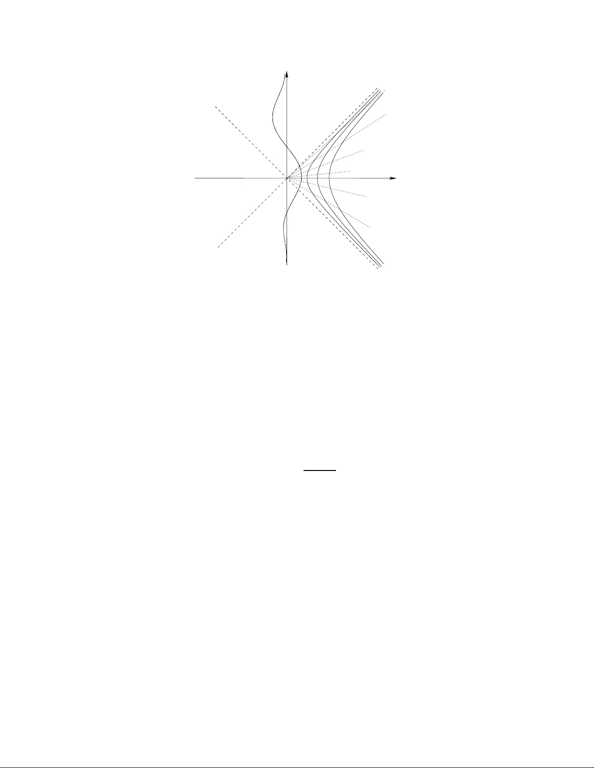
Relativistic i n variance of L yapuno v exponents in bounded and unbound ed systems Adilson E. Motter 1 and Alberto Saa 2 1 Department of Physics and Astr onomy , Northwestern University , Evanston, IL 60208, USA 2 Department of Applied Mathematics, UNICAMP , C.P . 6065, 13083-859 Campin as, SP , Brazil (Dated: Nov ember 13, 2018 ) Abstract The s tudy of chaos in relati vistic systems has been hampered by the observ er depend ence of L yapu nov exp onents (LEs) and of condition s, such as orbit boundedn ess, in v oked in the interp retatio n of LEs as indica tors of chaos. Here we establish a general framewo rk that ov ercomes both dif ficulties and apply the resulti ng appro ach to address three fundamenta l questio ns: how LEs trans form under Lorentz and R indler transfo rmations and under transformat ions to uniformly rotating frames. The answers to the first and third questi ons show that inertial and uniformly rotating observ ers agree on a charact erizati on of chaos based on LEs. The second ques tion, on the other hand, is an ill-po sed problem due to the eve nt horizo ns inheren t to unifor mly accelerated obser ver s. P A CS numbers: 05.45.- a, 95.10 .Fh, 98.80.Jk 1 The quest for an observer -independent characterization o f chaos in relativistic systems [1] has been an i ntense area of research and promi ses to provide signi ficant new insights into the properties of chaoti c dynamics [2]. An import ant recent resul t [3] concerns t he t ransformation of L yapunov exponents (LEs) under s pacetime diffe omorphism s. W e recall that the d ynamics of a bounded solution X ( t ) of a dynamical system d X dt = F ( X ) (1) is chaotic if it presents sensit iv e dependence on initi al condi tions [4]. The associated L Es [5] are given by λ i = lim s up t →∞ 1 t log || ϕ i ( t ) || , where ϕ i ( t ) are solutions o f the linearized equation d dt ϕ i = [ D X F ( X ( t ))] ϕ i . Positive LEs are related to exponential diver gence of i nitially close trajectories and, consequently , to chaotic dynamics. For sp ace d iff eomorphisms X = Ψ ( Y ) , the in variance of the LEs is well established under rather general condit ions (see, e.g., [6, 7]). In contrast, for well-behaved spacetime diffeomorphisms in volving tim e changes of the form dτ = Λ( X ) dt , it has been shown [3] th at the LEs transform according to λ τ i = λ t i / h Λ i t , (2) where 0 < h Λ i t < ∞ is the time a ve rage of Λ alo ng the corresponding trajectory . Therefore, although the values of the LEs are themselves no n-in variant, t heir signs are p reserved and assure an in v ariant criterion for chaos un der spacetime transform ations. This result was obtained und er conditions for which LEs are known to be valid quantifiers of chaos, of which the most limiti ng ones are the assumptions that the system has a natural in var iant probability measure and the orbits are bounded both before and after the transformation. In this Letter , we e xtend t his result to an important class of transform ations that do not preserve the boundedness of the orbits, and a ddress fundamental questions on relativistic chaotic dynamics that require explicit in-depth in vestigat ion due to thei r outstandi ng physical properties and the violation of cond itions in v oked in the deriva tion of Eq. (2). The first question is how the LEs transform un der Lorent z transformation s. This qu estion d etermines whether all inertial observers agree on a LE-based characterization of chaos. W e show that t he answer is af firmati ve despite the fact that t he dynamics becomes unbounded with respect to at least one of the reference frames. W e use thi s e xample to establi sh an extended boundedness condition for the definition of the LEs as indi cators of chaos, which is form ulated relati ve to t he t rajectories th emselves rather than a fixe d point of the phase space. The second qu estion is h ow th e LEs behave under Rindler transformations, a question equiv alent to ask whether uniformly accelerated observers agree on an 2 inertial characterization o f chaos based on LEs. W e show t hat t his question is ill-pos ed because uniformly acc elerated observer s do not ha ve access to the late-time dynami cs. The latter relates to the fact that chaos and LEs are asymp totic concepts [8] wh ose definition s in v olve a limit t → ∞ . W e also consider transformations to uniformly rotating frames, and show that the positivity of the LEs remains in v ariant under such t ransformations. Our princi pal result stems from this analys is and can be stated for an y system and any spacetime diffeomorphic transformation , as follows. For the sys tem writt en in aut onomous form, the LEs transform according to Eq. (2) and remain in var iant indicators of chaos if, as sho w n belo w , ( i ) our extended boundedness condition is satisfied, ( ii ) the Jacobian of the transformati on is bounded, and ( iii ) Λ is positive for all t and 0 < h Λ i t < ∞ . These conditions depend not only on the transformation pro perties of the dynami cal variables X and the change of reference frames but also on the choice of spacetim e coordinates. They are autom atically satisfied for global nonsin gular transformations of boun ded orbits for which inf Λ ± 1 > 0 whether the system is conservativ e, dissipative, mechanical, chem ical, thermodyn amical, electromagnetic, or fluid dynamical. Th ese conditions clarify previous results [9] that seem t o challenge the in var iance of chaos for relativistic observers, and sho w that LEs lead to i n variant conclusions about chaos. W e fi rst note that under a space dif feomorphism X = Ψ ( Y ) , system (1) is mapped into d dt Y = [ D Y Ψ ( Y )] − 1 F ( Ψ ( Y )) , rendering the solutions of the new linearized dynam ics to be related to those of (1) as ϕ i ( t ) = [ D Y Ψ ( Y ( t ))] ˜ ϕ i ( t ) [7]. Hence, the corresponding LEs satisfy lim inf t →∞ 1 t log || [ D Y Ψ ( Y ( t ))] ˜ ϕ i ( t ) || || ˜ ϕ i ( t ) || ≤ λ i − ˜ λ i ≤ lim sup t →∞ 1 t log || [ D Y Ψ ( Y ( t ))] ˜ ϕ i ( t ) || || ˜ ϕ i ( t ) || . (3) Suppose the solutions X ( t ) ar e limited to a compact subset of the space. Since the diffemorphism maps bounded solutions X ( t ) into bounded solutions Y ( t ) , the matrix D Y Ψ ( Y ( t )) is nonsingular and, besides, there are time-independent finite nonzero constants L ± = sup || [ D Y Ψ ( Y ( t ))] ± 1 || leading to lim t →∞ 1 t log 1 L − ≤ λ i − ˜ λ i ≤ lim t →∞ 1 t log L + , (4) which imply ˜ λ i = λ i [7]. Thi s ar gum ent e xplores the boundedness of X ( t ) and Y ( t ) to ensure the existence of the constants L ± . Belo w we extend ( 4) and establish Eq. (2) for an important class of unbounded orbits. W e now consider transformations o f reference frame in wh ich (1) describes a bo unded au- tonomous system with respect to th e initial (inertial ) observers. More general transformations can be obtai ned by a compositio n of s uch t ransformations. W e start with single-particle sy stems. 3 While general relativity allows arbitrary spacetime coordinates, and cond itions ( i - iii ) can be ap- plied to any of them, we will assu me that the dynami cs is described in terms of physical t imes (i.e., t he time m easured by observers at rest in the reference frame at the correspon ding space coordinates). Lor entz transformations. W e first focus on t he case in which function F depends o nly on the configuration-space coordinates, su ch as in the e volution of a fluid element determin ed by a stream function, a nd consider a Lorentz boost w ith velocity v along the x -direction, ( ct, x, y , z ) → ( ct ′ , x ′ , y ′ , z ′ ) = Ψ − 1 ( ct, x, y , z ) , where Ψ − 1 ( ct, x, y , z ) = ( γ ( ct − v x/c ) , γ ( x − v t ) , y , z ) (5) for γ = 1 / p 1 − ( v /c ) 2 . W e focus on the space spanned by the coordinates ( ct, x, y , z ) ≡ ( ct, x ) , where we ha ve enlarged the configuration space in order t o incorporate ct as a ne w coordinate. The extended v ersion of (1) then reads d dt   w x   =   c F ( x )   , (6) where dw /dt ≡ d ( ct ) /dt . The main adv antage o f this formulation is that the transformed system remains autonomous and the spacetime transform ation can be reduced t o an ordinary space di ff eomorphism; it can be split as T ◦ S ( ct, x ) , wh ere S is a transformation ( w ′ , x ′ ) = Ψ − 1 ( w , x ) that preserv es the independent var iable and T is a tim e redefinition dt ′ = Λ( w , x ) dt . (Another adva ntage is that the analysis extends im mediately to F with explicit tim e-periodic d ependence.) The sol utions of (6) are u nbounded alon g th e w -direction, b ut t his is not a probl em since the n onzero LEs of system (6) are identical to those of (1). There is a ca veat, howe ver: the spatial boundedness of the solut ions is no t p reserved under Lorentz transformations. A trajectory confined to a bounded space-like re gion ( sup || x ( t ) || < ∞ ) of the first reference frame is seen as spatially unbounded from the other inertial reference frame. Similar probl em is obs erved e ven for Galilean transformation s, but in classi cal dynami cs one can adopt a reference frame where th e solution s are bounded. In relati vistic dynamics such a choi ce would raise questions about the in variance of the LEs, which is precisely th e object of this Letter . T o proceed we first m ake the crucial observation that the study of chaos can be extended t o this class of spatially unbo unded orbits , ev en though the same does not hold true for unb ounded 4 systems in general. Indeed, sensiti ve dependence on initial con ditions and LEs depend e xclusively on t he relati ve time ev olution between nearby trajectories; their dependence on the reference frame is limited to the definition of the spacetime coordinates used to measure the distances between the neighboring trajectories as they ev olve over i dentical t ime int erv als. Therefore, chaos can be properly defined and LEs can be used as indi cators of chaos on an unb ounded trajectory y ( t ) insofar as || y ( t ) − ˆ y ( t ) || r emains unifor mly upper bounded for all t and all trajectories ˆ y ( t ) with initial conditions in a neighbo rhood of y (0) . That is, our condition is that the e v olution of a small ball of poin ts wil l remain bounded wi th respect to the local observers at positio n y ( t ) , regar dless of whether it remains bounded with respect to a fix ed point of the reference frame. W e refer to t his as the extended boundedness conditio n. N ote that thi s condition is sati sfied for y ( t ) interpreted as the e xtended c oordinates ( w ′ ( t ) , x ′ ( t ) ) after the tra nsformation S whenev er the origin al system (1) is spatially bounded. Ha ving shown that LEs remain valid indicators of chaos despit e t he spatial u nboundedness o f the transformed orbits , we now turn to the eff ect of the L orentz transformations on t he LEs. F or the transformation T , from Eq. (5) we hav e dt ′ = γ  1 − v c 2 F x ( x ( t ))  dt ≡ Λ ( x ( t )) dt, (7) where F x ( x ) stands for th e x -component of F ( x ) . For | F x ( x ( t )) | ≤ c , im plying inf Λ( x ( t )) > 0 in the present case, we hav e 0 < h Λ i t = lim t →∞ t ′ ( t ) t = lim t →∞ 1 t R t 0 Λ( x ( p )) dp < ∞ [10]. This allows us to factor the LEs transformed by T ◦ S as ˜ λ t ′ i = ˜ λ t i / h Λ i t , (8) where h Λ i t is t he contribution due to T and ˜ λ t i corresponds to λ t i transformed by S . The problem is thus r educed to the transformation of the LEs under the spatial transformati on S . The nonsingular nature of (5) assu res th e existence of the cons tants L ± necessary to establ ish the bound s i n (4) because, irrespecti ve of the spati al unbound edness, the Jacobian matrix o f the transform ation is bounded. Employing the Euclidean n orm to the mat rix D y Ψ ( y ) o f (5), we obtain L + = L − = p ( c + | v | ) / ( c − | v | ) , leading to ˜ λ t i = λ t i . In particular , all po sitive LEs remain posit iv e under this transformation. Combined with Eq. (8), this results in ˜ λ t ′ i = λ t i / h Λ i t , which is precisely the transformation (2) pre viously establish ed for the case of bounded orbits [3]. Our result does no t agree with the result presented in [9] for ave rages ov er l ocal LEs [11], b ut that is bec ause that study was restricted 5 to time dilatations and length contractions, which correspond to the transformation of dynamical var iables su ch as v olume (or the reciprocal of a density) for the t ime m easured at a fixed po int of the reference frame, whereas our analysis describes single-particle dynamics for the tim e measured at the position of the particle. If syst em (1) in volve s the ev olution of velocities, as expected for a particle in a 3D po tential, the Lorentz transformation (5) must be extended to incl ude the transform ation of u ≡ d x /dt into u ′ ≡ d x ′ /dt ′ , which is given by u ′ x = η ( u x − v ) , u ′ y = η γ − 1 u y , and u ′ z = η γ − 1 u z , where η = 1 / (1 − u x v /c 2 ) . The resul ting transformati on ( w , x , u ) → ( w ′ , x ′ , u ′ ) sati sfies the extended boundedness conditi on and has constants 0 < L ± < ∞ , as long as | v | < c and | u x ( t ) | ≤ c . This ensu res th at the LEs o f sy stems obtained by order reduction of second-order di ff erential equations, which are t he most common in particle dynam ics, will be transformed as in (2) under Lorentz transformations. Rindler transformations. W i th respect to an inertial reference frame, an observer with con- stant proper acceleration a along the x direction has a hyperbolic w orldline giv en by ct ( τ ) = c 2 a sinh aτ c , x ( τ ) = c 2 a cosh aτ c , (9) where τ stands for the observer’ s proper tim e. The corresponding Rindl er transformation [12] is defined by ( ct, x, y , z ) → ( cτ ( t, x ) , ξ ( t, x ) , y , z ) , with ct ( τ , ξ ) = c r 2 ξ a sinh aτ c , x ( τ , ξ ) = c r 2 ξ a cosh aτ c , (10) and positive ξ (see Fig. 1). Th e observer on hyperbole (9) is in th e Rindler reference frame at rest at ξ = c 2 / 2 a . In cont rast wi th the Lorentz case, the Rindler transformations are non-li near in x and ct . Focusing on t he space defined by t he extended configuration-space coordinates, the m atrix D y Ψ ( y ) and i ts in verse for the Rindler transform ation of (6) hav e u nit determinants but t heir lar gest eigen values diver ge as c/ √ 2 aξ cosh aτ /c for ξ → 0 . Therefore , on e cannot ident ify fi- nite const ants L ± that could b e used t o compare ˜ λ t i and λ t i . This behavior can be interpreted in terms of our extended boun dedness condition, which is not satisfied in this case because ( cτ ( t, x ( t )) , ξ ( t, x ( t )) , y ( t ) , z ( t )) diver ges at the light cone and is und efined beyond it. Moreover , from the in verse of Eqs. (10 ), we ha ve dτ = c 2 a  x ( t ) − tF x ( x ( t )) x ( t ) 2 − ( ct ) 2  dt ≡ Λ( ct, x ( t )) dt, (11) 6 ct II III I IV Event horizon Γ ο ο (ξ=0, τ= ) ο ο − (ξ=0, τ= ) x FIG. 1: Accessibility to the dynamics is observer dependent. The lines of fixed ξ in R indler coordin ates corres pond to hyperbolic trajectorie s in the coo rdinat es ( ct, x ) of inertial observ ers. T he straigh t dotted l ines are the lines of consta nt time τ . The uniformly accelera ted observe rs are unaware of all e ven ts occur ring in regions II and III of the original Minko wski spacetime. T hey only access the dynamics of a trajectory Γ during the time the traject ory crosses regi on I [13]. If the trajector y is spatially bound ed with respect to the origin al observ ers , as assumed for system (1), this correspo nds to an infinite time interv al ∆ τ bu t only to a finite time interv al ∆ t . where Λ( ct, x ( t )) diver ges when t he orig inal s olution ( ct, x ( t )) crosses the li ght cone x 2 = c 2 t 2 . The same holds true for the physical time dt ′ = p 2 aξ /c 2 dτ . The a verage h Λ i t is not well defined and, as a result , the Rindler transformed s ystem does not hav e a natural probability measure against which the LEs could be calculated [3]. Therefore, the question of how the LEs transform under Rindler transformations is ill-posed. The real origin of the problem is th e horizon structu re (and its counterpart structure fo r t → − t ) inherent to un iformly accelerated observers [12 ]. Th e Rindl er transformation (10) is not a gl obal spacetime dif feomorphism since it m aps onl y one quarter of th e M inkowski spacetime, as shown in Fig. 1. Any e vent located abov e the component of the light cone corresponding to t he bisectrix in the first and third quadrants of Minkowski sp acetime will ne ver r each the accelerated observers. While s ingularities can b e an artifact of the coordin ates, event horizons are an attribute of th e reference frame. The existence o f an e vent horizon prevents the observers from having access to the asymptotic dynamics of the original system . Therefore, without ha ving acce ss to the complete 7 dynamics, t he Rindler observers cannot formulate a criterion for chaotic behavior —based on the observation of individual trajectories—that is v alid for t he origi nal s ystem [13]. It is interesting to notice that such a problem , related to the global structure of the spacetime, manifests itself as a violation of our conditions for the transformation of LEs. If one insist s on computing the LEs from a uniformly accelerated referential frame [9], o ne must note that th e late-time dy namics of the extremely dilated tim e τ → ∞ does no t correspond t o the real late-time dynamics of the original system since the i nterval −∞ < τ < ∞ is the mappi ng of a finite tim e interval ∆ t . T herefore even if one could compu te ˜ λ τ i as seen from th e accelerated frame, this would be, in fact, a p roblem different from the originally proposed one. This situation is analogous t o the li mits imposed by t he cosmolog ical si ngularity to t he determination of chaos in FR W cosmo logies [8] and is also predicted for Rindler transformations of any other dynamical system and for any choice of coordinates. Rotating frames. The crucial rol e played by the e vent horizon in the R indler case can be better appreciated if o ne considers a ph ysical situation in v olving a non-linear transform ation that does not introduce event horizons. This is precisely the case of uniformly rotating reference frames [14]: r ′ = r , θ ′ = θ + Ω t , z ′ = z , and cdt ′ = [ g ( r ) + Ω 2 r 2 /g ( r )] dt + [Ω r 2 /g ( r )] dθ , where g ( r ) = √ c 2 − Ω 2 r 2 , Ω is a constant, and t ′ is the physical time in the rotating frame [15]. Thi s leads to dt ′ =  g ( r ( t )) c + Ω r 2 ( t )[Ω + F θ ( x ( t ))] cg ( r ( t ))  dt, (12) where F θ ( x ) = dθ /d t . The transform ation of the L Es of (6) is in this case well defined since the extended bou ndedness condit ion is satisfied for orbit s in closed sets of the physical region | Ω | r < c for wh ich − Ω r 2 F θ ( x ) < c 2 , where both the function Λ( x ) and the constants L ± are upper and lowe r b ounded aw ay from zero. The latter follows from the fact t hat t he entries of the Jacobian matrix D y Ψ ( y ) and its in verse for the transformation ( ct, r , θ , z ) → ( ct ′ , r ′ , θ ′ , z ′ ) are all con tinuous for Ω r < c . A s ubtlety in this calculation is that i n rotati ng frames the differ ential dt ′ of the physical t ime is not exact and cannot be integrated globally , m eaning that the Jacobian elements in v olving deriv ati ves of ct ′ must be determined from cdt ′ in the immediate neighborhood of a given r . Th e transformation t → t ′ is defined locally but it can always be e xtended along any trajectory with initial condition i n that n eighborhood. Therefore, the LEs transform as predicted by (2) also for the case of rotating frames. Generalization and discussion. Ou r deriv ation of Eq. (8) also demonstrates that condi tions ( i - iii ) are sufficient (and usually necessary) for the validity of (2) in general. Indeed, whi le we 8 considered specific transformations and specific class es of dynamical systems in our explicit ex- amples, these three conditions are precisely the checkpoints we hav e to verify for any sy stem and any transformatio n. The extended boundedness condition— satisfied both before and af ter the transformation in the extended space , which includes ct as an addit ional coordinate—guarantees that the s ystem can b e kept aut onomous and t hat LEs remai n v alid in dicators of chaos. The con- dition that the Jacobian is bounded—in t he sense of having pos itive finite constants L ± for the transformation in t he ex tended space —ens ures the validity of the ident ity ˜ λ t i = λ t i . Finally , Λ and h Λ i t positive and finite—again, in th e e xtended space —guarantees that the ti me transformation is well defined and the signs of the LEs ar e c onserved; it also guarantees that the time transformation is in vertible, a condition we saw violated for the Rindler transformation. These condition s are readily applicable to any system and any change of reference frame and coordinates. The latt er includes the choice of the time parameter or of the observers in the reference frame with respect to which the time is measured. In the examples above, the dynamical system describes t he dynamics of a single particle, the dynami cal v ariables repre- sents the coordinates and possibly velocities of the particle, and the time was assumed to be recorded locally —each ti me by the observer in the reference frame t hat is at the point where the particle is. Howe ver , oth er choices are equall y v alid. F or a m any-particle system under Lorentz transformation , for example, the time coul d be measured, e.g., with respect to the po- sition of one of the particles, d t ′ = γ  1 − v c 2 F x i ( x ( t ))  dt , with respect to the center of mass, dt ′ = γ  1 − v c 2 P i m i P j m j F x i ( x ( t ))  dt , or with respect to a fix ed point, dt ′ = γ dt . Moreover , the dynamical system can describ e phys ical, chemical or biological activity whose dynam ical vari- ables do not necessarily correspond t o coordinates and velociti es in t he physical space. In this general case the s ystem can be writ ten as d dt X i = F i ( X 1 , . . . X n ) , i = 1 , . . . n , and the transforma- tion is locally defined as ( cd t, d X 1 , . . . d X n ) → ( cd t ′ , d X ′ 1 , . . . d X ′ n ) . The latter is determined by the change of reference frame and s pacetime coordinates, ( cdt, d x ) → ( cdt ′ , d x ′ ) , and depends on t he nature of the dynam ical variables, i.e., whether t hey transform as s calars, vectors, t ensors, or in a differ ent way . Th e choice of observers in the new reference frame is always accounted for through the c hoice of d dt x in the transformation formula dt ′ =  ∂ ∂ t t ′ ( ct, x ) + ∇ x t ′ ( ct, x ) · d dt x  dt , where this term vanishes only if the tim e is measured (remotely) by a fix ed observer . The results presented in this Letter a ddress all these cases and show that, if conditio ns ( i-i ii ) are verified, the signs of the LE s remain valid in variant indicators of chaos. Since we have extended the use of the LEs as a v alid measure of chaos to include unbounded orbits, this conclusion is general: 9 it appl ies to bo th inertial and non-inertial reference frames and does no t in volv e the ident ification of privileged observers. These results account for properties inherent to relativistic observers, such as e vent h orizon and spatial unboundedness , significantly e xtending our understanding of the relativistic in v ariance of LEs and chaos. The authors thank E. Gu ´ eron, G. M atsas and R. V enegeroles for insi ghtful di scussions. Thi s work was supported by F APESP and CNPq. [1] G . Francisc o and G. E. A. Matsas, Gen. Relati v . Gra vit. 20 , 1047 (1988). For an early revie w , see D. Hobill, A. Burd, and A . Cole y (Eds.), Deterministic C haos in Genera l R elativi ty (Plenum P ress, New Y ork, 1994). [2] P . Cipriani an d M. D i Bari, Phy s. Rev . L ett. 81 , 55 32 (1998); L. Horwitz et al . , ibid 98 , 234301 (2007). [3] A . E. Motter , P hys. Re v . Lett. 91 , 231101 (2003). [4] E . Ott, Chaos in Dynamica l Systems (Cambridg e U ni v . P ress, Cambridg e, 1994). [5] V . I. Oseledec, Tr ans. Mosco w Math. Soc. 19 , 197 (1968 ). [6] R . Jaros lawsk i et al. , Z. Phys. B 82 , 437 (1991 ). [7] R . Eichhor n, S . J. Linz, and P . H ¨ anggi, Chaos, Solitons & Fractals 12 , 1377 (20 01). [8] A . E. Motter and P . S. Letelier , P hys. Re v . D 65 , 068502 (2002). [9] Z . Zheng, B. Misra, and H. Atmanspach er , Int. J. Theor . Phys. 42 , 869 (2003). [10] Similarly , 0 < h Λ i − 1 t = h Λ − 1 i t ′ = lim t ′ →∞ t ( t ′ ) t ′ < ∞ . [11] B. Eckhard t and D. Y ao, Physica D 65 , 100 (1993); S. V . Ershov and A . B. Potapov , ibid 118 , 167 (1998 ); P . Gaspard, Chaos, Scatte ring and Statistica l Physics (Cambridg e Univ . Press, Cambridge , 1998) . [12] C. de A lmeida and A. Saa, Am. J. Phys. 74 , 15 4 (2006). [13] In pri nciple, th ey can remot ely o bserv e t he dynamics fo r t < 0 and determine the backward LE s based on that informati on. [14] J. R. Letaw and J. D. Pfautsch , Phys. Rev . D 22 , 1345 (1980); J. Math. Phys. 23 , 425 (1982). [15] R. J. Cook, A m. J. Phys. 72 , 21 4 (2004). 10