Rate and power allocation under the pairwise distributed source coding constraint

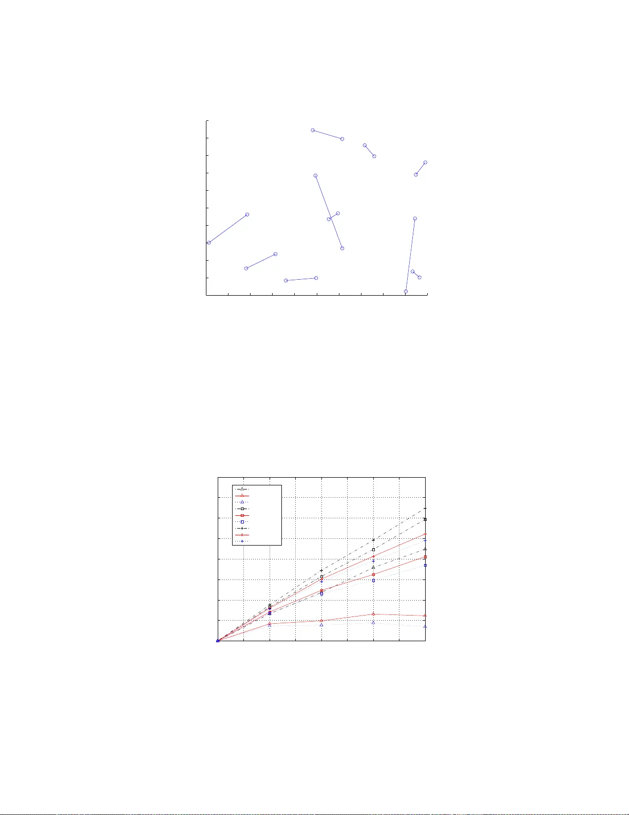
1 Rate and po wer alloca tion und er the pairwise distrib uted source coding constraint Shizheng Li and Adi tya Ramamoorthy Department of Electrical and C omputer Engineering Io wa State Univ ersity Ames, Iow a 50011 Email: { sz li, adityar } @iastate.edu Abstract W e consider the problem of rate an d power allocation fo r a sensor network und er the pair wise distributed so urce coding constraint. For noiseless source- terminal chan nels, we show that the m inimum sum rate assignment can be found by finding a minimum weight arborescen ce in an appropr iately defined directed graph . For orthogo nal noisy sou rce-termina l channels, the minimum sum power alloca tion can be found by finding a minimum weight matching forest in a mixed graph. Numerical results are presented for both cases showing that our solu tions alw ays outperfo rm previously propo sed solutio ns. The gains are considerable when source co rrelations are high. Index T erms distributed source co ding, Slepian-W o lf theo rem, matchin g forest, dire cted span ning tree, resource allocation The material in this wo rk was presented in part at the IE EE Intl. Symp. on Info. Th. 2008. This r esearch was supported in part by NSF grant CNS-0721453. Nov ember 9, 2018 DRAFT I . I N T R O D U C T I O N The av ailability of low- cost sensors h as enabled th e emer g ence of lar ge-scale sensor networks in recent years. Sensor networks typically consist of sensors that hav e li mited power and are moreover energy constrained since they are us ually battery-operated. The data t hat is sensed by senso r networks and com municated to a terminal 1 is usually correlated. Thus, for sensor networks it is im portant to allocate resources such as rates and power by taking the correlation into account. The famous Slepian-W olf theorem [1] s hows that the di stributed compression (or distributed sou rce coding) o f correlated sources can in fact be as effic ient as joint compressio n. Coding techni ques that approach the Slepian-W olf bound s hav e been in vestigated [2] and their usage proposed in sensor networks [3]. T ypicall y on e wants to m inimize metrics such as the total rate or tot al power expended by t he sensors in such situations . A number of authors ha ve considered problems of this fla vor [4], [5], [6]. These papers assume th e existence of Slepian- W olf codes that work for a lar ge number of sensors. In practice, the design of low-complexity Slepian-W olf codes is well understood on ly for the case of two sources (denoted X and Y ) and th ere have been constructions that are able to operate on the boun dary of th e Slepian-W olf region. In particular , the desi gn of codes (eg.[7],[8],[9]) is easiest for the corner point s (asymmetric Slepian-W olf codin g) where the rate pair is either ( H ( X ) , H ( Y | X )) or ( H ( X | Y ) , H ( Y )) . Severa l sym metric code designs are proposed in [10],[11],[12] i n which the authors main ly focus on two correlated sources. In [7], the correlation between two bi nary sources are assumed to be sym metric and the LDPC code is designed for a virtual BSC correlation channel, while the codes designed in [9], [10] and [11] are su itable for arbit rary correlation between the two bin ary sources. The authors of [13] p roposed code designs for mult iple sources. For two uni formly di stributed bi nary s ources whose correlation can b e model ed as a BSC channel, their design sup ports both symmetri c and asymmetric codin g and approaches Slepian-W olf bound. Howe ver , when it comes to more than 1 W e shall use terminal and sink interchangably through out this paper . 2 two sources, in order t o achiev e opt imum rate (joint entropy), they hav e a strong assumptio n on correlation model, i.e., the correlation between all the sources is solely d escribed by their modulo-2 sum. Thus, giv en the current state of the art in code design it is of interest to consider coding strategies for sensor networks where pairs of nodes can be decoded at a time instead of all at once. This observation was made in the work of Roumy and Gesbert i n [14]. In th at work th ey formul ated the pairwise distri buted source coding problem and p resented algorithms for rate and p owe r allocation under different scenarios. In particular , th ey cons idered t he case when there exist di rect channels between each source nod e and th e termi nal. Furthermore, the terminal can only decode t he so urces pairwise. W e briefly revie w their work below . The work of [14] considers two cases. i) Case 1 - Noiseless node-terminal channels. Under t his scenario, they considered the prob lem of deciding which particular nodes should be decoded to gether at the terminal and their corresponding rate allocations s o t hat t he to tal sum rate is m inimized. ii) Case 2 - Ort hogonal noisy node-terminal channels. In t his case the channels were assumed to be noisy and orthogonal and the objective was to d ecide which nod es would be paired so that overall power consumption is m inimized. In [14], the problem was m apped ont o the problem of choosing the mi nimum weight matching [15] of an appropriately defined weighted undirected graph. Each node participate in joi nt decoding only once. In t his paper we consider a class of p airwise distri buted source coding solutions t hat is larger than the ones considered in [14 ]. The basi c idea i s t hat previously decoded data can be used as side informat ion for ot her sources. A simple example demonstrates that it is not necessary to only consider m atchings Consider four correlated sources X 1 , X 2 , X 3 and X 4 . The s olution of [14] constructs a complete graph on the four nodes X 1 , . . . , X 4 and assigns th e edge weights as the joi nt entrop ies i.e. the edge ( X i , X j ) is assigned weigh t H ( X i , X j ) . A mi nimum wei ght matching algorithm is then run on this graph to find the mini mum sum rate and the rate allocation. 3 Suppose that this yields the m atching ( X 1 , X 3 ) and ( X 2 , X 4 ) so that the s um rate becomes 4 X i =1 R i = H ( X 1 , X 3 ) + H ( X 2 , X 4 ) . Since conditioning reduces entropy , it i s si mple to obs erve that H ( X 1 , X 3 ) + H ( X 2 , X 4 ) ≥ H ( X 1 ) + H ( X 3 | X 1 ) + H ( X 2 | X 3 ) + H ( X 4 | X 2 ) . W e no w show that a n alternativ e rate allocation: R 1 = H ( X 1 ) , R 2 = H ( X 2 | X 3 ) , R 3 = H ( X 3 | X 1 ) and R 4 = H ( X 4 | X 2 ) can still allow pairwise decoding of th e sources at the termi nal. Note th at at the decoder we hav e, a) X 1 is k nown since R 1 = H ( X 1 ) . b) X 3 can be recovered by jointly decoding for X 3 and X 1 since X 1 is kno wn and the decoder has access to H ( X 3 | X 1 ) amount of data. c) X 2 can be recove red since X 3 is known (from above) and the decoder h as access to H ( X 2 | X 3 ) amou nt o f data. d) Similarly , X 4 can be recov ered. As we see above, the sources can be decoded at the terminal in a pipelined manner . Note that we can lever age the coding solut ions proposed for two sources at the corner point s in th is case since the encoder for X 3 can be desi gned ass uming t hat X 1 is known perfectly , the encoder for X 2 can be designed assuming that X 3 is known perfectly etc. The method of source-splitti ng [16], [17] is closely related to th is approach. Given M sources and an arbitrary rate point in their Slepian-W olf region, i t con verts the problem into a rate allo cation at a Slepian-W olf corner point for appropriat ely defined 2 M − 1 so urces. Howe ver as pointed out b efore, code designs e ven for corner poi nts are not that well understood for mo re than two sou rces. Thus, while using source-splitting can result in sum -rate opt imality i.e. the sum rate is the joi nt entropy , i t may not be very practical giv en the current state of the art. Moreover , for M sou rces it requires the design of approximately twice as many encoders and more decoding sub-modules that also comes at t he cost o f complexity . 4 In this paper , m otiv ated by complexity is sues, we present an alt ernate formulation of the pairwise distri buted source cod ing problem that is more general than [14]. W e demonst rate that for nois eless channels the minimu m sum rate all ocation problem becomes one o f finding a minimum weight arborescence of an appropriately defined directed graph. Next, we show that in the case of noisy channels, the m inimum sum power all ocation problem can be mapped onto finding the m inimum weight matchi ng forest of an appropriately defined mixed graph 2 . Simulation results show that our solutio ns are sign ificantly better than t hose in [14] i n the cases when correlations are hi gh. This paper is organized as follows. W e form ulate t he problem and briefly revie w previous solutions based on matchi ng in Section II. In Section III and IV we present our solut ion for noiseless channels and no isy channels respectiv ely . Numerical result s for the both cases are giv en in Section V and Section VI conclu des this paper . I I . P RO B L E M F O R M U L A T I O N A N D OV E RV I E W O F R E L A T E D W O R K Consider a set of correlated sources X 1 , X 2 , . . . , X n transmittin g data t o one sink in a wireless sensor network. W e ass ume t hat ev ery source can transmit d ata directly to the t erminal. The source X i compresses its data at rate R i and sends it t o the sink. W e assume that the sources encode only their own dat a. Furthermore, we consider the class of s olutions where the sink can recov er a given source with the help o f at most one ot her source. The problem has two cases. i) Case 1 - Noiseless node-terminal channels. Assume that there is no no ise i n t he channel. In order t o reduce the storage requirement at the sens ors, we want to minim ize the sum rate, i.e., min P n i =1 R i . ii) Case 2 - Ort hogonal noisy node-terminal channels. Assume that channels bet ween sou rces and sink are corrupted by additive white Gaussian noise and there is no internode int erference. In this case, sou rce channel separation holds [18]. The capacity of th e channel bet ween node i and the s ink with transmissio n power P i 2 A mixed graph has both directed and undirected edges 5 and channel g ain γ i is C i ( P i ) , log(1 + γ i P i ) , w here noise power is normalized to one and channel gains are constants known to the terminal. Rate R i should satisfy R i ≤ C i ( P i ) . Let [ n ] denote the ind ex set { 1 , . . . , n } . The transm ission p ower is constrained by peak power constraint: ∀ i ∈ [ n ] , P i ≤ P max . In this context, our objectiv e is to mini mize the sum power , i .e., min P n i =1 P i . Note t hat i n the impl ementation from t he practical poin t of vi e w , we can us e joint distributed source codin g and channel coding [19 ], [20], on ce the pairing of nodes i n volved in join tly d ecoding are known from the resource allocation solut ion. W e now overvie w the work of [14]. For noiseless case, i n order for the terminal t o recov er data perfectly , the rates for a pair of nodes i and j shoul d be in the Slepian and W olf region S W ij , { ( R i , R j ) : R i ≥ H ( X i | X j ) , R j ≥ H ( X j | X i ) , R i + R j ≥ H ( X i , X j ) } . Note that H ( X i , X j ) i s the minim um sum rate whil e i and j are paired to perform joint d ecoding. The matching solution of the problem is as follows. Construct an und irected compl ete graph G = ( V , E ) , where | V | = n . L et W E ( i, j ) denote weight on und irected edge ( i, j ) , W E ( i, j ) = H ( X i , X j ) . Then, find a minimum weight m atching P of G . For ( i, j ) ∈ P , the o ptimal rate allocation ( R i , R j ) can be any point o n the slope of th e SW region of nodes i and j since they g iv e same s um rate for a pair . W e can simply s et ( R i , R j ) for ( i, j ) ∈ P to be eith er ( H ( X i ) , H ( X j | X i )) or ( H ( X j ) , H ( X i | X j )) , i .e., at the corner points o f SW region. For noisy case, the rate region for a pair of nod es is the intersection of SW region and capacity region C ij : C ij ( P i , P j ) , { ( R i , R j ) : R i ≤ C i ( P i ) , R j ≤ C j ( P j ) } . It i s easy to see that for a node i with rate R i and p owe r P i , at the opti mum R ∗ i = C i ( P ∗ i ) , i.e. the inequality R i ≤ C i ( P i ) constraint is met with equality . Thus, the power ass ignment is given by the in verse function of C i which we d enote by Q i ( R i ) , i.e., P ∗ i = Q i ( R ∗ i ) = (2 R ∗ i − 1) / γ i . T his problem can also be solved by finding min imum m atching on a undirected graph. Howe ver the weights in this case are the minimum sum power for each pair of nod es. The sol ution has two steps: 1) Find opt imal rate-power allocati ons for all possi ble no de pairs: ∀ ( i, j ) ∈ [ n ] 2 s.t. i < j : ( R ∗ ij ( i ) , R ∗ ij ( j )) = arg min Q i ( R ij ( i )) + Q j ( R ij ( j )) (1) 6 s.t. ( R ij ( i ) , R ij ( j )) ∈ S W ij ∩ C ij ( P max , P max ) (2) The power allocations are giv en by P ∗ ij ( i ) = Q i ( R ∗ ij ( i )) and P ∗ ij ( j ) = Q j ( R ∗ ij ( j )) . Th e rates R ij ( i ) , R ij ( j ) are the rates for node i and node j when i and j are paired. Note th at when i and anoth er node k 6 = j are consid ered as a pair , the rate for i m ay be diff erent,i.e., R ij ( i ) 6 = R ik ( i ) . 2) Construct an undirected com plete graph G = ( V , E ) , where W E ( i, j ) = P ∗ ij ( i ) + P ∗ ij ( j ) for edge ( i, j ) , and find a mini mum matching P in G . The power allocation for no de pair ( i, j ) ∈ P denoted b y ( P i , P j ) i s ( P ∗ ij ( i ) , P ∗ ij ( j )) and the correspondin g rate allocation can be found. The solution for step (1) i s given in [14] and d enoted as ( P ∗ ij ( i ) , P ∗ ij ( j ) , R ∗ ij ( i ) , R ∗ ij ( j )) . This solution is the opti mum rate-po wer all ocation between a p air of nodes i and j under the peak power constraint and SW region constraint. Note that in t his case, the rate assignment s for i and j do not necessarily happen at the corner of the SW region. I I I . N O I S E L E S S C A S E As s hown by the example in Section I, the rate all ocation given by matching may not be optimum and i n fact there exist o ther schemes that hav e a lower rate while s till working with the current coding solut ions to t he two source SW problem. W e now present a formal definition of the pairwi se decoding constraint. Definition 1 : P airwise pr opert y of rate assignment. Consider a set of dis crete memoryless sources X 1 , X 2 , . . . , X n and th e corresponding rate assign ment R = ( R 1 , R 2 , . . . , R n ) . The rate assignment is said to satisfy th e pairwise p roperty if for each source X i , i ∈ [ n ] , there exists an ordered sequence of sources ( X i 1 , X i 2 , . . . , X i k ) such that R i 1 ≥ H ( X i 1 ) , (3) R i j ≥ H ( X i j | X i j − 1 ) , for 2 ≤ j ≤ k , and (4) R i ≥ H ( X i | X i k ) . (5) 7 Note that a rate assi gnment that satisfies the pai rwise p roperty allows the possi bility that each source can be reconstructed at the decoder by solvi ng a sequence of decoding operations at the SW corner points e.g. for decoding so urce X i one can use X i 1 (since R i 1 ≥ H ( X i 1 ) ), then decode X i 2 using the knowledge of X i 1 . Continuing in this manner finally X i can be decoded. A rate assign ment R shall be called pairwise valid (or valid in this section), if it satisfies th e pairwise property . In this section, we focus on lo oking for a valid rate allo cation that mi nimizes the sum rate. An equiv alent definition can be given in graph-theoretic terms by constructi ng a graph called th e pairwise property test graph correspon ding to th e rate assi gnment. P airwise Property T est Graph Constructio n 1) Input s : t he number of nodes n , H ( X i ) for all i ∈ [ n ] , H ( X i | X j ) for all i, j ∈ [ n ] 2 and the rate assignment R . 2) Initi alize a graph G = ( V , A ) wit h a total of 2 n nodes i.e. | V | = 2 n . Th ere are n re gula r nodes denoted 1 , 2 , . . . , n and n starred n odes deno ted 1 ∗ , 2 ∗ , . . . , n ∗ . 3) Let W A ( j → i ) denote th e weight on directed edge ( j → i ) . For each i ∈ [ n ] : i) If R i ≥ H ( X i ) then insert edge ( i ∗ → i ) with W A ( i ∗ → i ) = H ( X i ) . ii) If R i ≥ H ( X i | X j ) then insert edge ( j → i ) wit h W A ( j → i ) = H ( X i | X j ) . 4) Remove all nodes that do not participate in any edge. W e denote the result ing graph for a giv en rate allo cation by G ( R ) = ( V , A ) . Note t hat if R is valid, the graph sti ll contains at least one s tarred node. Next, based o n G ( R ) we define a set of n odes that are called the parent nodes. Parent ( R ) = { i ∗ | ( i ∗ → i ) ∈ A } , i .e., Parent ( R ) corresponds to the s tarred nodes for the set of sources for which the rate allocatio n i s at least the entropy . Mathematically if i ∗ ∈ Parent ( R ) , t hen R i ≥ H ( X i ) . W e now demonstrate the equiv alence between the pairwi se property and t he const ruction of the graph above. Lemma 1: Consider a set of discrete correlated s ources X 1 , . . . X n and a correspond ing rate assignment R = ( R 1 , . . . , R n ) . Const ruct G ( R ) based o n th e algorith m above. Th e rate assign- ment R satisfies the pairwise p roperty if and only i f for all regular nod es i ∈ V there exists a starred node j ∗ ∈ Parent ( R ) such that there exists directed path from j ∗ to i in G ( R ) . 8 Pr oof: Suppose that G ( R ) is such t hat for all regular nodes i ∈ V , there exists a j ∗ ∈ Parent ( R ) so that there is a directed path from j ∗ to i . W e show that this impli es the pairwi se property for X i . Let t he path from j ∗ to i be denot ed j ∗ → j → α 1 . . . → α k → i . W e note that R j ≥ H ( X j ) by const ruction. Similarly edge ( α l → α l +1 ) exists in G ( R ) only because R α l +1 ≥ H ( X α l +1 | X α l ) and like wise R i ≥ H ( X i | X α k ) . Thus for source i we have found the ordered sequence of sources ( X j , X α 1 , . . . , X α k ) that satisfy properties (3), (4) and (5) in d efinition 1. Con versely , if R satisfies the pairwise property , then for each X i , there exists an ordered sequence ( X i 1 , . . . , X i k ) th at satis fies properties (3), (4) and (5 ) from definition 1. This implies that th ere exists a d irected pat h from i ∗ 1 to i in G ( R ) , since ( i ∗ 1 → i 1 ) ∈ A because R i 1 ≥ H ( X i 1 ) and furthermore ( i j − 1 → i j ) ∈ A because R i j ≥ H ( X i j | X i j − 1 ) , for j = 2 , . . . , k .  W e define another set of g raphs that are useful for presenting t he m ain result of this section. Definition 2 : Specification of G i ∗ ( R ) . Suppos e that we construct graph G ( R ) as above and find Parent ( R ) . For each i ∗ ∈ Parent ( R ) we construct G i ∗ ( R ) in the following mann er: For each j ∗ ∈ Parent ( R ) \{ i ∗ } remove the edge ( j ∗ → j ) and the n ode j ∗ from G ( R ) . For the next result we need to introd uce the concept of an arborescence [15]. Definition 3 : An arb or escence (also cal led dir ected spanning t r ee) of a di rected graph G = ( V , A ) rooted at vertex r ∈ V is a s ubgraph T o f G such that it is a spanning tree if the orientation of the edges is ignored and there is a pat h from r to all v ∈ V when the direction of edges is taken int o account. Theor em 1: Consider a set of d iscrete correlated sources X 1 , . . . , X n and let the corresponding rate assig nment R be pairwise valid. Let G ( R ) be cons tructed as above. T here exists another valid rate assi gnment R ′ that can be described by the edge weights of an arborescence of G i ∗ ( R ) rooted at i ∗ where i ∗ ∈ Parent ( R ) such that R ′ j ≤ R j , for all j ∈ [ n ] . Pr oof: W e sh all show that a new subgraph can be cons tructed from which R ′ can be obtained. This shall be done by a series of graph-t heoretic transformat ions. Pick an arbitrary starred node j ∗ ∈ Parent ( R ) and construct G j ∗ ( R ) . W e claim that in the current graph G j ∗ ( R ) th ere exists a path from th e st arred node j ∗ to all regular nod es i ∈ [ n ] . 9 T o see this note that since R is pairwise valid, for each regular node i there exists a path from some starred n ode to i in G ( R ) . If for some regular nod e i , t he starred node is j ∗ , the path is still i n G j ∗ ( R ) . Now consid er a regular node i 1 and suppose there exists a directed path k ∗ → k → β 1 . . . → i 1 in G ( R ) where k ∗ ∈ Parent ( R ) , k ∗ 6 = j ∗ . Since k ∗ ∈ Parent ( R ) , R k ≥ H ( X k ) ≥ H ( X k | X l ) ∀ l ∈ [ n ] . This implies that edge ( l → k ) i s i n G j ∗ ( R ) , ∀ l ∈ [ n ] , in particular , ( j → k ) ∈ G j ∗ ( R ) . Therefore, in G j ∗ ( R ) there exists the path j ∗ → j → k → β 1 . . . → i 1 . This claim implies that there exists an arborescence rooted at j ∗ in G j ∗ ( R ) [15]. Suppose we find such one such arborescence T j ∗ of G j ∗ ( R ) . In T j ∗ e very node except j ∗ has exactly one i ncoming edge (by the property of an arborescence [15]). Let inc ( i ) denote t he node such t hat ( inc ( i ) → i ) ∈ T j ∗ . W e define a new rate assignm ent R ′ as R ′ i = W A ( inc ( i ) → i ) = H ( X i | X inc ( i ) ) (for i ∈ [ n ] and i 6 = j ), and R ′ j = W A ( j ∗ → j ) = H ( X j ) . The existence of edge ( j ∗ → j ) ∈ G ( R ) impl ies R ′ j = H ( X j ) ≤ R j . Similarly , we hav e R ′ i ≤ R i for i ∈ [ n ] \{ j } . And it is easy to see that R ′ is a valid rate assignment .  Thus, the above theorem impli es that v ali d rate assignments that are described on arborescence s of the graphs G i ∗ ( R ) are th e best from the point of v iew of mini mizing the sum rate. Finally we ha ve the fol lowing t heorem that says that the va lid rate assignment that mini mizes the sum rate can be found by finding m inimum weig ht arborescences o f appropriately d efined graphs. For the statement of the theorem we need to define the fol lowing g raphs. a) T he graph G tot = ( V tot , A tot ) is such t hat V tot consists of n regular nodes 1 , . . . , n and n starred nodes 1 ∗ , . . . , n ∗ , | V tot | = 2 n . The edge set A tot consists of edges ( i ∗ → i ) , W A ( i ∗ → i ) = H ( X i ) for i ∈ [ n ] and edges ( i → j ) , W A ( i → j ) = H ( X j | X i ) for all i, j ∈ [ n ] 2 . b) For each i = 1 , . . . , n we define G i ∗ as the graph obtained from G tot by del eting all edges of the form ( j ∗ → j ) for j 6 = i and all nodes in { 1 ∗ , . . . , n ∗ }\{ i ∗ } . Theor em 2: Consider a set of sou rces X 1 , . . . , X n . Suppose that we are interested in finding a valid rate assignm ent R = ( R 1 , . . . , R n ) for these sources s o that the su m rate P n i =1 R i is 10 minimum . Let R i ∗ denote the rate assi gnment specified by the m inimum weigh t arborescence of G i ∗ . Then t he optimal valid rate assi gnment can be found as R opt = arg min i ∈{ 1 ,...,n } n X j =1 R i ∗ j Pr oof. From Theorem 1 we hav e that any valid rate assi gnment R can b e transformed into new rate assignment t hat can be described on an arborescence of G i ∗ ( R ) rooted at i ∗ and s uitable weight assignment . It is component -wise lower than R . This impli es th at i f we are i nterested in a min imum sum rate soluti on, it s uffi ces to focus our attenti on on so lutions specified by all solutions that can be described by all possi ble arborescences of graphs of the form G i ∗ ( R ) over all i ∗ = 1 ∗ , . . . , n ∗ and all p ossible valid rate assi gnments R . Now consi der the graph G i ∗ defined abov e. W e not e th at all graphs of the form G i ∗ ( R ) where R is valid are subgraphs of G i ∗ . Therefore finding t he mini mum cost arborescence of G i ∗ will yield us t he best rate assignment possible within the class of so lutions specified b y G i ∗ ( R ) . Next, we find the best solutions R i ∗ for all i ∈ [ n ] and pick the so lution with t he minimum cost. This yields the opt imal rate ass ignment.  I V . N O I S Y C A S E In this section we con sider the case when the sources are connected to the termi nal by orthogonal nois y channels. In this case, the objective is to mi nimize the sum p ower . Therefore the optim um rate allo cation w ithin a pair of s ources may not be at the corner points of SW region. W e want some node pairs working at corner poin ts whil e some others working on the slope of the SW region. T aking this i nto account, we generalize the concept of pairwise property . For a given rate assignm ent R , w e say that X i is in itially decodabl e if R i ≥ H ( X i ) , or together w ith ano ther source X j , ( R i , R j ) ∈ S W ij . If R i ≥ H ( X i ) , it can be d ecoded by itself. If ( R i , R j ) ∈ S W ij , SW codes can be d esigned for X i , X j and they can be recovered by joint decoding. In addit ion, if we take advantage of previously decoded source data to help decode other sources as we did in the nois eless case, starting with an i nitially decodable sou rce, more sources can potentially be recov ered. 11 Definition 4 : Generalized p airwise pr oper ty of rate assignment. Consider a set o f discrete memoryless sources X 1 , . . . , X n and t he corresponding rate assignm ent R = ( R 1 , . . . , R n ) . The rate assign ment is said to s atisfy the generalized pairwise property if for each X i , i ∈ [ n ] , X i is initially decodable, or there exists an ordered sequence of sources ( X i 1 , X i 2 , . . . , X i k ) such that X i 1 is i nitially decodable , (6) R i j ≥ H ( X i j | X i j − 1 ) , for 2 ≤ j ≤ k . (7) R i ≥ H ( X i | X i k ) (8) A rate assignment R s hall be call ed generalized pairwise valid (or valid in this section), if it satisfies the generalized pairwise property and for e very rate R i ∈ R , Q i ( R i ) ≤ P max . A valid rate assignm ent allows e very source to b e recov ered at the sink. A power ass ignment P = ( P 1 , P 2 , . . . , P n ) shall be called valid, if t he corresponding rate ass ignment i s valid. W e s hall introduce generalized pairwise p roperty test graph. The inp ut and initializati on are the same as p airwise prop erty test g raph construction. Th en, for each i ∈ [ n ] : i) If R i ≥ H ( X i ) then insert di rected edg e ( i ∗ → i ) with weight W A ( i ∗ → i ) = Q i ( H ( X i )) . ii) If R i ≥ H ( X i | X j ) then insert directed e dge ( j → i ) with weight W A ( j → i ) = Q i ( H ( X i | X j )) . iii) If ( R i , R j ) ∈ S W ij , then insert undirected edge ( i, j ) with weight W E ( i, j ) = Q i ( R ∗ ij ( i )) + Q j ( R ∗ ij ( j )) = P ∗ ij ( i )+ P ∗ ij ( j ) . Note that as pointed out in Section II, ( P ∗ ij ( i ) , P ∗ ij ( j ) , R ∗ ij ( i ) , R ∗ ij ( j )) are t he optimum rate-po wer allocatio n between nod e p air ( i, j ) giv en by [14]. Finally , remove all nodes that do n ot participate i n any edge. W e denote the result ing graph for a given rate allocati on by G M ( R ) = ( V , E , A ) , where E is undirected edge set and A is directed edge set. Denot e the regular node set as V R ⊂ V . Lemma 2: Consider a set of discrete correlated s ources X 1 , . . . X n and a correspond ing rate assignment R = ( R 1 , . . . , R n ) . Suppose that we construct G M ( R ) based on th e algo rithm above. The rate assig nment R i s generalized pairwise valid if and only if, ∀ R i ∈ R , Q i ( R i ) ≤ P max , and for all regular nodes i ∈ V R , at least o ne of these condi tions ho lds: 1) i participates in an und irected edge ( i, i ′ ) , i ′ ∈ V R ; 2) There exists a starred node i ∗ and an directed edge ( i ∗ → i ) ; 12 3) There exists a starred node j ∗ such t hat there is a di rected path from j ∗ to i ; 4) There exists a regular node j participatin g in edge ( j, j ′ ) , j ′ ∈ V R such that there is a directed path from j to i ; The pro of of this lemma is very simi lar to t hat of Lemma 1. If one of the conditio ns 1) and 2 ) holds, X i is ini tially decodable, and vice versa. If one of the conditi ons 3) and 4) holds, X i can be decoded in a sequence of decoding procedures which starts from an ini tially decodable s ource X j , and vice versa. Next, we i ntroduce som e definitio ns crucial to the rest of the development. Definition 5 : Giv en a mixed graph G = ( V , E , A ) , if e = ( i → j ) ∈ A , i is the t ail and j is the head of e . If e = ( i, j ) ∈ E , we call both i and j the head of e . For a node i ∈ V , h G ( i ) denotes the number o f edges for which i is the head. Definition 6 : The underlying undir ected graph of a mixed g raph G deno ted by U U G ( G ) is the undirected graph obtained from the mixed graph by forgetting the o rientations of the directed edges, i.e., treating di rected edg es as undirected edges. As pointed out previously , we want som e nodes to work at corner point s of two-dimensio nal SW region and others to work on the slope. Thus, we need to somehow combine the two concepts of arborescence and matching. The appropriate concept for our purpose is the notion of a matching forest first in troduced in the work of Giles [21]. Definition 7 : Giv en a m ixed graph G = ( V , E , A ) , a subg raph F of G is called a matching for est [21] if F contains no cycles in U U G ( F ) and any node i ∈ V is t he head of at most one edge in F , i.e. ∀ i ∈ V , h F ( i ) ≤ 1 . In t he context of t his section we also define a strict matching forest. For a mi xed g raph G containing regular nodes and starred nodes, a matching forest F satisfyin g h F ( i ) = 1 , ∀ i ∈ V R (i.e. every regular node is the head of exactly one edg e) is called a strict m atching for est(SMF) . In the no isy case, th e SMF pl ays a role si milar to the arborescence in the noiseless case. Now , we introduce a t heorem similar t o Theorem 1. Theor em 3: Given a g eneralized pairwis e valid rate assignment R and corresponding power assignment P , let G M ( R ) be construct ed as above. There exists another valid rate assi gnment 13 R ′ and power assignment P ′ that can be described by the edge weights of a strict matching forest of G M ( R ) such that P n i =1 P ′ i ≤ P n i =1 P i . Pr oof. In order to find such a SMF , we first change the weight s of G M ( R ) , yielding a new graph G ′ M ( R ) . Let W ′ A ( i → j ) , W ′ E ( i, j ) denote weights i n G ′ M ( R ) . Let Λ be a sufficiently large constant. W e perform the following weight transformation on all edges. W ′ E ( i, j ) = 2Λ − W E ( i, j ) , W ′ A ( i → j ) = Λ − W A ( i → j ) . (9) Denote the sum weight of a subgraph G ′ of graph G ′ M ( R ) as W t G ′ M ( R ) ( G ′ ) . Next, we find a maximum weight matching forest of G ′ M ( R ) .which can be done in polynomial time [22]. Lemma 3: The maximum weight m atching forest F M in G ′ M ( R ) is a st rict matchin g forest, i.e., it satisfies: ∀ i ∈ V R , h F M ( i ) = 1 . Pr oof. See Appendix. Note that each re gular node is head of exact one edge in F M . The power allocation is performed as fol lows. Any i ∈ V R is the head of one o f three ki nds of edges in F M corresponding t o t hree kinds of rate-powe r assig nment: 1) If ∃ ( i ∗ → i ) ∈ F M , then set P ′ i = Q i ( H ( X i )) and R ′ i = H ( X i ) . The existence o f edge ( i ∗ → i ) in G M ( R ) means that R i ≥ H ( X i ) , so R ′ i ≤ R i and P ′ i ≤ P i ≤ P max . 2) If ∃ ( i, j ) ∈ F M , set P ′ i = P ∗ ij ( i ) , R ′ i = R ∗ ij ( i ) and P ′ j = P ∗ ij ( j ) , R ′ j = R ∗ ij ( j ) . The existence of edge ( i, j ) in G M ( R ) means that R i and R j are in t he SW region, P i ≤ P max and P j ≤ P max . W e know that P ∗ ij ( i ) , P ∗ ij ( j ) i s the mini mum sum power sol ution for node i and j wh en the rate allocation is in SW region and the power allo cation satisfies P max constraints. So P ′ i + P ′ j ≤ P i + P j , P ′ i ≤ P max , P ′ j ≤ P max . 3) If ∃ ( j → i ) ∈ F M , set P ′ i = Q i ( H ( X i | X j )) and R ′ i = H ( X i | X j ) . The existence of edge ( j → i ) in G M ( R ) means th at R i ≥ H ( X i | X j ) , so R ′ i ≤ R i and P ′ i ≤ P i ≤ P max . Therefore, the new power allo cation P ′ reduces the sum power . Notice th at when we are assigning new rates to the nodes, the conditio ns in Definition 4 st ill hol d. So the new rate R ′ is also valid. So P ′ is a valid p ower allo cation wi th l ess sum power .  14 The following theorem says that the valid p ower assignm ent that mi nimizes the s um power can be found by finding minimum weigh t SMF of an appropriately d efined g raph. The graph G tot = ( V tot , A tot , E tot ) is such that V tot consists n regular nodes 1 , . . . , n and n starred no des 1 ∗ , . . . , n ∗ , and | V tot | = 2 n . The directed edge set A tot consists of edg es ( i ∗ → i ) , W A ( i ∗ → i ) = Q i ( H ( X i )) for { i : i ∈ [ n ] and Q i ( H ( X i )) ≤ P max } , and directed edges ( i → j ) , W A ( i → j ) = Q j ( H ( X j | X i )) for { i, j : i, j ∈ [ n ] 2 and Q j ( H ( X j | X i )) ≤ P max } . The undirected edg e s et E tot consists o f edges ( i, j ) , W E ( i, j ) = P ∗ ij ( i ) + P ∗ ij ( j ) for all i, j ∈ [ n ] 2 . Assume that P max is large enoug h so that there exist at least one valid rate-power allocation , the following th eorem shows that the op timal rate-power allocati on can be found in G tot . Theor em 4: Consider a set of sou rces X 1 , . . . , X n . Suppose that we are interested in finding a valid rate assignment R and it s corresponding power assignment P for these sources s o that the sum power P n i =1 P i = P n i =1 Q i ( R i ) is mi nimum. The optim al valid power assign ment can be specified by th e minimum weigh t SMF of G tot . The proof of thi s t heorem is similar to that of Theorem 2. Note t hat matching i s a special case of matching forest, and is also a special case of SMF in our problem. Th erefore, minim um weight SMF s olution i s always no worse than mi nimum matchin g sol ution. W e n ow show that the minimu m SMF i n G tot can be found by findi ng maximum matching forest in another mixed graph after weight transformation. W e can perform the same weight transformation for G tot as we did for G M ( R ) . Denote the resulting graph as G tot ′ . Find the maximum weight m atching forest F ′ M in G tot ′ . Denote th e corresponding m atching forest in G tot as F M . W e claim that both F ′ M and F M are SMFs. T o see this, not e that since there exists valid rate allocation R , G ′ M ( R ) is a subgraph of G tot ′ . From Lemma 3, we know that SMF exists i n G ′ M ( R ) . Therefore, SMF also exists in G tot ′ . Because in a SMF starred n ode is not head o f any edge and regular node is head of exact one edge, based on weight transformation rules, t he weight of a SMF F ′ S in G tot ′ is: W t G tot ′ ( F ′ S ) = n Λ − W t G tot ( F S ) (10) where F S is the corresponding SMF in G tot . W eight of any non -strict matching forest F N S 15 is W t G tot ′ ( F ′ N S ) = m Λ − W t G tot ( F N S ) , m < n . Since Λ is s uffi ciently large, W t G tot ′ ( F ′ S ) > W t G tot ′ ( F ′ N S ) , i.e., SMFs in G tot alwa ys hav e larger weights . Therefore, the maxi mum wei ght matching forest F ′ M in G tot ′ is SMF . So i s the correspond ing matching forest F M in G tot . From (10), i t is easy to see i n G tot the matching forest correspond ing to F ′ M (the m aximum weight matching forest i n G tot ′ ) has minimum wei ght, i.e., F M is t he minimum SMF in G tot . V . N U M E R I C A L R E S U L T S W e cons ider a wireless s ensor network example in a square area where the coordi nates of the sensors are randomly chosen and uniforml y d istributed in [0 , 1] . The sou rces are assum ed to be jointly Gaussian distributed such that each s ource has zero mean and unit variance (this model was also used i n [23]). The off-diagonal elements of the covariance matrix K are given by K ij = exp( − cd ij ) , where d ij is t he distance between n ode i and j , i .e., the nodes far from each oth er are less correlated. The parameter c indicates t he spatial correlation in the data. A l ower va lue of c indi cates hi gher correlation. The individual entropy of each s ource is H 1 = 1 2 log(2 π eσ 2 ) = 2 . 05 . Consider the noiseless case first. Because the rate allo cation only d epends on entropi es and conditional entropies, we do not need to care the location of the s ink. It is easy to see b ased on our assum ed model that H ( X i | X j ) = H ( X j | X i ) , ∀ i, j ∈ [ n ] 2 . Thus, W A ( i → j ) = W A ( j → i ) . It can be s hown that the weight s of m inimum weight arborescences G i ∗ , i = 1 , . . . , n are th e same. Therefore, we only need to find m inimum weight arborescence on G 1 ∗ . A solu tion for a sensor network containing 20 nodes are shown in Fig.1. Since the starred node 1 ∗ is vi rtual in the network, we did not pu t it on the graph. Instead, we marked node 1 as root in the arborescence, whose t ransmission rate is its individual entropy H 1 . Edge ( i → j ) in the arborescence implies that X i will be decoded in adv ance and used as side information to help decode X j . The matching solution for the same network i s shown in Fig.2. As no ted in [14], the optimu m m atching tries to match close neighbors together because H ( X i , X j ) decreases with the i nternode dist ance. Our arborescence s olution also showed simi lar property , i .e., a node tended to help its close n eighbor 16 since the conditi onal entropies b etween them are small . In Fig.3 , we plot the normalized sum rate R s 0 , P n i =1 R i /H 1 vs. the number of senso rs n . If there is n o pairwise decoding, i.e., the nodes transmi ts data i ndividually to t he sink, R i = H 1 and R s 0 = n . The m atching solution and the minimum arborescence (M A) solution are com pared in t he figure. W e also plotted the op timal norm alized su m rate H ( X 1 , . . . , H n ) /H 1 in the figure. The rate can be achiev ed theoretically when all sources are jointl y decoded together . W e obs erve that if the nodes are highly correlated ( c = 1) , the present soluti on ou tperforms the m atching soluti on cons iderably . Even if the correlation is not high , our M A sol ution is always better than matching solution. It is int eresting to not e that even though we are doing p airwise distributed source coding, our su m rate is qui te close to the theoretical li mit whi ch is achiev ed by n -dimension al distributed source coding. Next, we consider optim izing the total power when there are A WGN channels between the sources and the sink. The channel gain γ i is the reciprocal of the square of the distance between source X i and t he si nk. W e assume th at the coordinates of the sink are (0 , 0) . An example of the strict matching forest (SMF) soluti on to a network with 16 sensors is given in Fig.4. There is one und irected edge in the SMF imply ing that the heads of this edge work on the slope of SW region. Other 14 edges are directed edges im plying that the t ails of the edges are us ed as side information t o help decode thei r heads. No node is encoded at rate H 1 . In fact, m ost minimu m SMFs i n our simulati ons exhibit this p roperty , i. e., the mini mum SMF cont ains 1 undirected edge and n − 2 directed edges between regular nodes. This f act coincides our intuition : transmitt ing at a rate of condit ional entropy i s t he m ost economi cal way , while transm itting at a rate of individual entropy consumes most power . The matching solution for the sam e network is given in Fig. 5. W e compare sum powers of t he SMF solution w ith matching solutio n in T able.I. Th e sum powers were a veraged over three realizatio ns o f sensor networks. W e also found t he theoretical optimal sum power when n -dim ensional dis tributed source coding is applied by solvin g the fol lowing con vex optimi zation problem. 17 min R 1 ,...,R n n X i =1 P i = n X i =1 (2 R i − 1) /γ i subject to (2 R i − 1) /γ i ≤ P max , ∀ i ( R 1 , . . . , R n ) ∈ S W n where S W n is t he n -dim ensional Slepian-W ol f region. From the t able, we can obs erve that our strategy alw ays outperforms the matching strategy regardless o f the level of correlation, and comes q uite close to the t heoretical limit that i s achieved by n -dimensional SW cod ing. V I . C O N C L U S I O N The op timal rate and power allocation for a s ensor n etwork under pairwise distributed source coding constraint was first introduced in [14]. W e proposed a more general definition of pairwise distributed source coding and provided solutio ns for the rate and po w er allocation problem, which can reduce the cost (s um rate or s um power) furth er . For the case when the so urces and t he terminal are connected by noiseless channels, we found a rate allocation with t he min imum sum rate given by t he minimu m weight arborescence on a well-defined directed graph. For noisy orthogonal s ource term inal channels, we found a rate-po wer allo cation wit h mini mum sum power given by the m inimum weig ht strict matching forest on a well-defined m ixed graph. All algorithms introduced have po lynomial-tim e com plexity . Numerical results show that our solution has significant gains over the solut ion in [14], especially when correlations are high. Future research directio ns would include extensions t o resource allocatio n problem s when joint decoding of three (or more) s ources [24] at one time is consi dered, in stead of onl y two in this paper . Ano ther i nteresting issue is t o consider interm ediate relay nodes i n t he network, which are able to copy and forward data, o r e ven encode data using network codin g [25]. V I I . A C K N OW L E D G E M E N T S The authors would like to thank t he anonymous re viewer s whose comm ents greatly im proved the quality o f the paper . 18 A P P E N D I X PR OOF OF LEMMA 3 W e shall first introdu ce and prove a lemma which facilitates the proof of Lemm a 3. Lemma 4: Consider two nodes i and j in a matching forest F such that either h F ( i ) = 0 or h F ( j ) = 0 , and they do not hav e incomi ng directed edges. Then, there does not exist a path o f the form i − α 1 − α 2 − · · · − α k − j (11) in U U G ( F ) . Pr oof. First consider t he case when h F ( i ) = h F ( j ) = 0 , i .e., i, j only have outgoi ng directed edge(s). Suppose there is such a path (11), edge ( i, α 1 ) should directed from i to α 1 in F since h F ( i ) = 0 , similarly , j → α k . As depicted in Fig.6, at least one node α l in the path will hav e h F ( α l ) = 2 . But we know th at h F ( t ) ≤ 1 holds for ev ery node t ∈ V in matching forest F . So there is n o such p ath (11) i n U U G ( F ) . If h F ( i ) = 0 , h F ( j ) = 1 and j connects to an undirected edge ( j, j ′ ) in F , i, j and j ′ can only have outg oing directed edge(s). By simi lar ar guments above, we kn ow that at least one node α l on the path is such th at h F ( α l ) = 2 . Similarly , the case w hen i connects to an u ndirected edge and h F ( j ) = 0 can be proved.  Pr oof of Lemma 3: W e wil l prove this lem ma by contradiction. W e shal l show that if h F M ( i ) = 0 for a regular node i , we can find another matching forest F ′ in G ′ M ( R ) such that W t G ′ M ( R ) ( F ′ ) > W t G ′ M ( R ) ( F M ) , i.e., F M is not the maxim um matching forest. Since F M is a matchi ng forest, it satisfies (a) h F M ( t ) ≤ 1 for ev ery node 3 t ∈ V and (b) no cycle exist in U U G ( F M ) . Suppose h F M ( i ) = 0 for a regular nod e i in F M . W e s hall make a set of mod ifications to F M resulting in a n e w matching forest F ′ and prove that these manip ulations will eve ntually i ncrease t he sum weight, make h F ′ ( i ) become 1 and ensure that there is no cycle in U U G ( F ′ ) . Al so, t hese modifications should guarantee that h F ′ ( j ) = 1 for j ∈ { j : j ∈ V R \{ i } and h F M ( j ) = 1 } , i.e. 3 Actually , for a star node i ∗ ∈ V \ V R , h F ( i ∗ ) = 0 in all matching forest F of G ′ M ( R ) because there is no incoming edge to i ∗ and i ∗ does not participate in an y undirected edge. 19 nodes that were previously the head o f som e edge continue to remain that way .During t he proof, we shall use the properties of G ′ M ( R ) giv en in Lemm a 2. Since R is valid, regular node i has at least one o f those four properties i n G ′ M ( R ) . W e shall discuss these cases in a more detailed manner: Case 1 . If t here exists a directed edge ( i ∗ → i ) in G ′ M ( R ) , add thi s edg e to F M to form F ′ . Clearly , W t G ′ M ( R ) ( F ′ ) > W t G ′ M ( R ) ( F M ) . Since there is only one out going edge from i ∗ and it has no incoming edge, no cycle in U U G ( F ′ ) is produced in our procedure. And h F ′ ( t ) ≤ 1 sti ll holds for e very node t ∈ V , so F ′ is still a matching forest. Case 2 . If th ere exists an un directed edge ( i, j ) i n G ′ M ( R ) , we can inclu de this edge to F M to increase sum w eight. Here, h F M ( i ) = 0 and there are two pos sibiliti es for h F M ( j ) , 0 or 1. Case 2a . If h F M ( j ) = 0 , add undi rected edge ( i, j ) to F M , resulting a new su bgraph F ′ . Obviously , the sum weight is increased whi le adding one edg e. Since h F M ( i ) = h F M ( j ) = 0 , b y Lemma 4 th ere does not exist path with form (11) in U U G ( F M ) . Thus, adding ( i, j ) does not introduce cycle in U U G ( F ′ ) . F ′ is a matching forest. Case 2b . If h F M ( j ) = 1 , we st ill add ( i, j ) but need to perform some preprocessing steps. Based on wh at kind of edge connects to node j , we have two cases: Case 2 b 1 . If there exists one directed edge ( j ′ → j ) in F M , delete edg e ( j ′ → j ) , we have an intermediate matchi ng forest F ′′ such t hat h F ′′ ( j ) = 0 . Add the undirected edge ( i, j ) to obtain F ′ . Not e that F ′ is a m atching forest because of arguments in Case 2a and W t G ′ M ( R ) ( F ′ ) > W t G ′ M ( R ) ( F M ) because for a s uf ficient large Λ , 2Λ − W E ( i, j ) > Λ − W A ( j ′ → j ) . Case 2 b 2 . If there exists one undirected edge ( j ′ , j ) in F M , we not ice th at the existence of ( j ′ , j ) i n G ′ M ( R ) in dicates that ( R j ′ , R j ) ∈ S W j ′ j , so R j ′ ≥ H ( X j ′ | X j ) and R j ≥ H ( X j | X j ′ ) , which impl ies that there exist di rected edges ( j → j ′ ) and ( j ′ → j ) i n G ′ M ( R ) . So w e can first delete edge ( j ′ , j ) and then add edges ( i, j ) and ( j → j ′ ) to form F ′ . Adding ( j → j ′ ) is to make sure h F ′ ( j ′ ) = 1 . Th ese modifications are shown in Fig.7. After removing edge ( j ′ , j ) , we hav e an intermediat e matchi ng forest F 1 such that h F 1 ( j ) = 0 and h F 1 ( j ′ ) = 0 . W e add edge ( i, j ) to obtain F 2 . Because of Lemma 4, F 2 is sti ll a m atching forest and h F 2 ( j ′ ) = 0 . 20 Then we add ( j → j ′ ) to ob tain a new subgraph F ′ . From Lemm a 4, we know that ( j → j ′ ) will not introduce cycle. Therefore, F ′ is st ill a matching forest. For a lar ge enough Λ , (2Λ − W E ( i, j )) + (Λ − W A ( j → j ′ )) > 2Λ − W E ( j, j ′ ) holds, so the s um weight will in crease. Case 3 . If there exist a path from h to i in G ′ M ( R ) : h → γ 1 → γ 2 → · · · → γ k 1 → i , where h is a starred node or participates in an undirected edge in G ′ M ( R ) , we use the foll owing approach. Note that γ 1 , . . . , γ k 1 may particip ate in undirected edges. On this path , w e find the node j closest to i such that j participates in an un directed edge in G ′ M ( R ) or it is a starred node. j m ay be the same as h or be s ome γ l . W e will focus on the path from j to i , denot ed by j → α 1 → α 2 → · · · → α k → i . The basic idea is to add edge α k → i into F M . Howe ver , if we just simply add t his edge, i t may produce cycle in underlying undirected graph. So we need more manipulatio ns. Case 3a . If j is a starred node, denote j as j ∗ , we want to add the path j ∗ → α 1 → α 2 → · · · → α k → i (12) to F M . First, in F M , remove al l incom ing directed edges to α l ( 1 ≤ l ≤ k ), then we hav e an i ntermediate m atching forest F 1 . Note t hat j ∗ , i , and α l ’ s only hav e outgo ing edges, by Lemma 4, we know that there does not exist undi rected path wit h the form j ∗ ( or α l 1 ) − β 1 − β 2 − · · · − β k − i ( or α l 2 ) in U U G ( F 1 ) where β ’ s are no des ou tside the path (12). Therefore, adding path (12) int o F 1 to form F ′ will not introduce a cycle. All nodes α l (1 ≤ l ≤ k ) on the p ath, h F ′ ( α l ) = 1 . F ′ is a matching forest. Next we s hall consider the weights. At some nodes, take α l for example, alt hough we deleted directed edge ( α l ′ → α l ) , where α l ′ is a node outside p ath (12), we add another directed edge ( α l − 1 → α l ) . T he weight m ight decrease by (Λ − W A ( α l ′ → α l )) − (Λ − W A ( α l − 1 → α l )) . Suppose we delete and add edges aroun d d nodes: α l 1 , α l 2 , . . . , α l d , the total weight decrease is P d i =1 W A ( α l i − 1 → α l i ) − W A ( α l i ′ → α l i ) . It may be po sitive but it d oes not contain a Λ t erm. At the end, we will add ( α k → i ) wi thout deleting any edge com ing int o i since h F M ( i ) = 0 , the weight will in crease (Λ − W A ( α k → i )) by t his operation. If Λ is large enough, the sum weight w ill finally increase. 21 Case 3b . If j participates in an u ndirected edge ( j ′ , j ) in G ′ M ( R ) . Note that j ′ 6 = α 1 , . . . , α k since j is th e first node i n the path t hat p articipates in an u ndirected edge. In this case, if ( j ′ , j ) is already in F M , we just need to add the path (12) from j t o i as we did in the case above to form F ′ . The resulti ng path is : j ′ − j → α 1 → α 2 → · · · → α k → i Note that i n F M , j ′ , j do not have directed incomin g edges. By simi lar argument in t he previous case, we know that F ′ is a matching forest. If ( j ′ , j ) is not in F M , we want to add ( j ′ , j ) to F M and then add the path (12). W e have fou r possibilit ies, some of which require preprocessing: Case 3 b 1 . h F M ( j ) = 0 and h F M ( j ′ ) = 0 ; we can add ( j ′ , j ) as we did in Case 2a, and then we add path (12) as we d id above. Case 3 b 2 . h F M ( j ) = 0 and h F M ( j ′ ) = 1 ; we can add ( j ′ , j ) after some preprocessing as we did in Case 2 b 1 and Case 2 b 2 , and th en we add path (12) as we did above. Next we dis cuss cases in which h F M ( j ) = 1 . In t his case, we only need to consid er some directed edge ( j ′′ → j ) comes into j in F M . If th ere some undirected edge ( j ′′ , j ) connecting j in F M , this case has been discussed in Case 3 b above, by treating j ′′ as j ′ . Case 3 b 3 . h F M ( j ) = 1 , ( j ′′ → j ) , and h F M ( j ′ ) = 0 ; W e can delete ( j ′′ → j ) and add ( j, j ′ ) as w e did in Case 2 b 1 , node j ′ is regarded as i in Case 2 b 1 , it is g uaranteed that t he resul ting subgraph is a matching forest. And t hen we add path (12 ) as we d id above. Case 3 b 4 . h F M ( j ) = 1 , ( j ′′ → j ) , and h F M ( j ′ ) = 1 ; For j ′ , it could be head of an undirected edge or a directed edge. If j ′ is head of an undirected edge ( j ′ , j ′′′ ) , we perform operations shown in Fig.8 t o get F ′ . The possibl e weight decrease during our operations around node j is ( W A ( j ′ → j ′′′ ) − W A ( j ′′ → j )) + (( W E ( j, j ′ ) − W E ( j ′ , j ′′′ )) . W e will add edge ( α k → i ) on p ath (12) wit h weight Λ − W A ( α k → i ) . Since Λ is large enough, the sum weight will still increase. If j ′ is head of a d irected edge ( j ′′′ → j ′ ) , we perform operations shown in Fig.9 to get F ′ . Similarly , because Λ is large enough , the sum weight will increase. R E F E R E N C E S [1] D. Slepian and J. W olf, “Noiseless coding of correlated information sources, ” IEEE T rans. on Info. Th. , vol. 19, pp. 471–48 0, Jul. 1973. 22 [2] S. S. P radhan and K. Ramchandran, “Distributed Source Coding using Syndromes (DISCUS): Design and C onstruction, ” IEEE T rans. on Info. Th. , vol. 49, pp. 626–6 43, Mar . 2003. [3] Z. Xi ong, A. D. L iv eris, and S. Cheng, “Distributed Source Coding for Sensor Networks, ” in IEEE Signal Pr ocessing Maga zine , Sept. 2004. [4] R. Cristescu, B. Beferull-Lozano, and M. V etterli, “On Network Correlated Data Gathering, ” in IEEE Infocom , 2004. [5] A. Ramamoorthy , “Minimum cost distributed source coding ov er a network, ” in IE EE Intl . Symposium on Info. Th. , 2007. [6] R. Cristescu, B. Beferull-Lozano, and M. V etterli, “Network ed slepian-wolf: theory , algorithms, and scaling laws, ” IEEE T rans. on Info. Th. , v ol. 51, no. 12, pp. 4057–4073 , Dec.2005. [7] A. L iv eris, Z. Xiong, and C. N . Georghiades, “Compression of binary sources with side information at t he decoder using LDPC codes, ” IEEE Comm. L etters , vol. 6, no. 10, pp. 440–442, 2002. [8] A. Aaron and B. Girod, “Compression with side information using turbo codes, ” in Pro c. I EEE Data Compr ession Confer ence(DCC) , 2002, pp. 252– 261. [9] D. Schonberg, S. S. Pradhan, and K. Ramchandran, “L DPC codes can approach the Slepian-W olf bound for general binary sources, ” in 40th A nnual A llerton Confer ence , 2002, pp. 576–585. [10] D. Schonberg , K. Ramchandran, and S. P radhan, “Distributed code constructions for the entire slepian-w olf rate region for arbitrarily correlated sources, ” in Pro ceedings. Data Compr ession Confer ence , 2004 . [11] V . T oto-Zarasoa, A. Roumy , and C. Guillemot, “Rate-adaptiv e codes for the entire slepian-wolf region and arbitrarily correlated sources, ” in IEEE International Confer ence on Acoustics, Speec h and Signal Pr ocessing(ICASSP) , 2008. [12] B. Bai, Y . Y ang, P . Boulanger , and J. Harms, “Symmetric Distributed Source Coding using LDPC Code, ” i n IEEE Int. Conf. on Comm. (ICC) , 2008, pp. 1892 –1897. [13] V . Stankovic, A. Live ris, Z. Xiong, and C. Georghiad es, “On code design for the slepian-wolf problem and lossless multiterminal networks, ” IEEE Tr ans. on Info. Th. , vol. 52, no. 4, pp. 1495–1 507, April 2006. [14] A. Roumy and D. Gesbert, “Optimal matching in wi reless sensor netwo rks, ” IEEE Journa l of Selected T opics in Signal Pr ocessing , vol. 1, no.4, pp. 725–735, Dec 2007. [15] J. Kleinber g and E. T ardos, Algorithm Design . Addison W esley , 2005. [16] B. Ri moldi and C. Urbanke, “Asynchron ous Slepian-W olf coding via source-splitting, ” in Proc. Intl. Symp. on Inf. Theory , Ulm, Germany , Jun.-Jul. 1997, p. 271. [17] T . P . Coleman, A. H. Lee, M. Medard, and M. Effros, “Lo w-complex ity approaches to Slepian-W olf near-lossless distrib uted data compression , ” IEEE Tr ans. on Info. Th. , vol. 52, no. 8, pp. 3546–356 1, 2006. [18] J.Barros and S.D.Servetto, “Network information flo w with correlated sources, ” IEEE T ran s. on Info. Th. , vol. 52, no. 1, pp. 155–1 70, 2006. [19] J. Garcia-Frias, Y . Zhao, and W . Zhong, “T urbo-Like Codes for Transm ission of Correlated S ources ov er Noisy Channels, ” IEEE Signa l Pr ocessing Magazine , vol. 24, no.5, pp. 58–66, 2007 . [20] W . Zhong and J. Garcia-Frias, “ LDGM Codes for Cha nnel Coding and Join t Source-Channel Coding of Correlated Sources, ” EURASIP J ournal on Applied Signal Processin g , vol. 2005, no. 6, pp. 942– 953, 2005. [21] R. Giles, “Optimum matching forests I: Special weights, ” Mathematical Pr ogramming , vol. 22, no. 1, pp. 1–11, Dec. 1982. 23 [22] ——, “Optimum matching forests II: General weights, ” Mathematical P r ogramming , vol. 22, no. 1, pp. 12–38, Dec. 1982. [23] R. Cristescu and B. Beferull-L ozano, “Lossy network correlated data gathering with high-resolution coding, ” IEEE T ransactions on Information Theory , vol. 52, no. 6, pp. 2817–2824, Jun. 2006 . [24] A. Liv eri s, C. Lan, K. Narayanan, Z . Xiong, and C. Georghiades, “Slepian-W olf coding of three binary sources using LDPC codes, ” in Pr oc. Intl. Symp. on T urbo Codes and Rel. T opics, Br est, F rance , Sep. 2003 . [25] R. Ahlswede, N. C ai, S.-Y . Li, and R. W . Y eung, “Network Information Flow, ” IEEE T rans. on Info. Th. , vo l. 46, no. 4, pp. 1204– 1216, 2000. Fig. 1. Minimum arborescence solution in a WSN with 20 nodes. Noiseless channels are assumed. Correlation parameter c = 1 . S um rate giv en by MA equals to 21.96, which is less than sum rate giv en by matching. The theoretical optimal sum rate is 20.54 . 24 0 0.1 0.2 0.3 0.4 0.5 0.6 0.7 0.8 0.9 1 0 0.1 0.2 0.3 0.4 0.5 0.6 0.7 0.8 0.9 1 Matching solution under noiseless channel: Sum Rate = 30.27 Fig. 2. Minimum matching solution in the same W SN as Fig.1. Noiseless channels are assumed. Correlation parameter c = 1 . Sum rate giv en by matching equals to 30.27. Note t hat if we do not take adv antage of correlation and transmit data indiv idually , the sum rate will be 20 × H 1 = 40 . 94 . 0 20 40 60 80 100 120 140 160 0 20 40 60 80 100 120 140 160 Number of sensors n Normalized sum rate R s0 c=1, Matching c=1, MA c=1, Optimal c=3, Matching c=3, MA c=3, Optimal c=5, Matching c=5, MA c=5,Optimal Fig. 3. Normalized sum rate vs. number of sensors 25 Fig. 4. Minimum strict matching forest solution in a WSN with 16 nodes. A WG N channels are assumed. Correlation parameter c = 1 . P eak power constraint P max = 10 . Sum power giv en by SMF equals to 16.27. The optimal sum power when we apply n -dimensional SW codes is 14.06. 0 0.1 0.2 0.3 0.4 0.5 0.6 0.7 0.8 0.9 1 0 0.1 0.2 0.3 0.4 0.5 0.6 0.7 0.8 0.9 1 Matching solution example for noisy channel, Sum power = 27.12 Fig. 5. Minimum matching solution in the same WSN as Fi g.4. A WGN channe ls are assumed. Correlation parameter c = 1 . Peak power constraint P max = 10 . Sum po wer giv en by matching equals to 27.12. Note that if we do not take adva ntage of correlation and transmit data indi vidually , the sum power wi ll be 47.11. 26 T ABLE I C O M PA R I S O N O F S U M P OW E R S B E T W E E N M I N I M U M S T R I C T M A T C H I N G F O R E S T A N D M AT C H I N G S O L U T I O N . P max = 10 . Number of nodes 4 8 12 c = 1 SMF 5.57 7.49 11.17 Matching 6.20 10.71 16.99 Optimal 5.45 7.06 9.93 c = 3 SMF 6.22 16.72 21.15 Matching 6.30 17.81 23.79 Optimal 6.17 16.44 20.60 c = 5 SMF 9.68 18.65 25.14 Matching 9.92 18.91 25.83 Optimal 9.67 18.56 24.96 i j i j a c D l D l D l+1 i j i j D l2 b D l D l+1 D v d D u D l1 Fig. 6. Case 2a: When h F M ( i ) = 0 , h F M ( j ) = 0 , path i − α 1 − α 2 − · · · − j can not exists in U U G ( F M ) because it will cause at lease one node α l , h F M ( α l ) = 2 . 27 i j j ‘ i j j ‘ i j j ‘ i j j ‘ F F 1 F 2 F ’ Fig. 7. Case 2 b 2 When h F M ( i ) = 0 , h F M ( j ) = 1 , ( j, j ′ ) ∈ F M , by introducing two intermediate matching forest F 1 , F 2 , we can find a ne w matching forest F ′ with l arger sum weight. j ’’ j j ’ j ’’’ j ’’ j j ’ j ’’’ F F ‘ i j ’’ j j ’ F 1 j ’’ j j ’ j ’’’ F 2 Fig. 8. Case 3 b 4 − 1 : When h F M ( j ) = h F M ( j ′ ) = 1 , ( j ′ , j ) ∈ G ′ M ( R ) , ( j ′′ → j ) ∈ F M , ( j ′ , j ′′′ ) ∈ F M , remove ( j ′′ → j ) to form an intermediate matching forest F 1 where h F 1 ( j ) = 0 , h F 1 ( j ′ ) = 1 , and ( j ′ , j ′′′ ) ∈ F 1 . Then apply the same operations as case (2 b 2 ) , resulting another matching forest F 2 . Finally add the path from j to i to get F ′ . 28 j ’’ j j ’ j ’’’ j ’’ j j ’ j ’’’ F F ‘ i j ’’ j j ’ j ’’’ F 1 j ’’ j j ’ j ’’’ F 2 Fig. 9. Case 3 b 4 − 2 : when h F M ( j ) = h F M ( j ′ ) = 1 , ( j ′ , j ) ∈ G ′ M ( R ) , ( j ′′ → j ) ∈ F M , ( j ′′′ → j ′ ) ∈ F M , remov e ( j ′′ → j ) to form an intermediate matching forest F 1 where h F 1 ( j ) = 0 , h F 1 ( j ′ ) = 1 , and ( j ′′′ → j ′ ) ∈ F 1 . Then apply the same operations as case (2 b 1 ) , resulting another matching forest F 2 . Finally add the path from j to i to get F ′ . 29