Nonvanishing boundary conditions and dark solitons in the NLS model

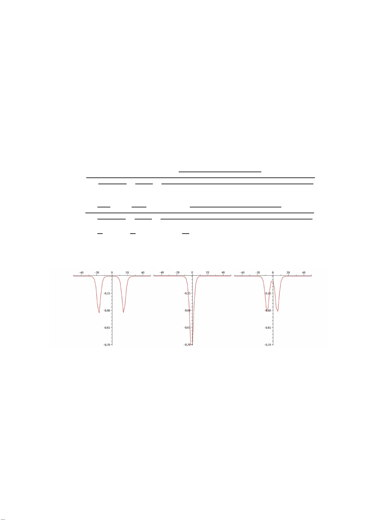
Non v anishing b oundary conditions and dark solitons in the NLS mo del 1 L.F. dos Sant os, H. Blas and M. J. B. F. da Silv a Instituto de F ´ ısica - Universidade F ederal d o Mato Gro sso Universidade F ederal de Mato Grosso Av. F ernando Co rrea, s/n, Co xip´ o 78060-900 , Cuiab´ a - MT - Brazil Abstract W e consider non-v anishing b ound ary conditions (NV BC) for the N LS mo del [1, 2, 3] in the context of the h ybrid dressing transformation and τ -function app roac h. In order to write the NLS mod el in a suitable form to deal with n on - v anishing b ou n dary conditions it is introduced a new sp ectral parameter in suc h a w a y that the usual NLS parameter will dep end on the affine parameter through t h e so-cal led Zuko wsky function. In the context of the dressing transformation t h e introd u ction of the affin e parameter a voids the construction of certain Riemann sheets for the usu al NLS spectral parameter. In this wa y one introduces a Lax p air defined for the n ew spectral parameter and th e relev ant NVBC NLS τ fun ct ions are obtained by the dressing transformation m eth od. W e construct the one and tw o dark-soliton solutions explicitly . 1 Po ster con tribution to the 5th Int ernational School on Field Theory and Grav itation, April 20 - 24, 2009, Cuiab´ a cit y , Brazil 1 The nonlinear Schroding er mo del (NLS) with v a nishing or non-v anishing b oundary conditions is physi- cally s ignificant since it appe ars in many applications rang ing from co ndensed matter to s tring theory (see e.g. [4]). The NLS mo del and its multifi eld extensions is an in tegrable sys tem (see e.g. [5] a nd references therein). Here w e provide the affine Ka c-Mo o dy algebraic for mulation of the NLS mo del suitably written for nonv anishing b oundary conditions and the hybrid of the dressing and Hiro ta methods is used to obtain dark soliton solutions of the model. The conv enien t form of the NLS for dealing with non-v a nis hing boundar y conditions, w hich suppor t dark-so liton like solutions [6], can be written as ∂ t ψ + ∂ xx ψ − 2 ( | ψ | 2 − ρ 2 ) ψ = 0 . (0.1) This form of NLS model is supplied with the non-v anishing boundar y conditions giv en b y [1, 2, 3] ψ =    ρ, x → − ∞ , ρǫ 2 , x → + ∞ ρ = r eal const. , ǫ = e iθ . (0.2) In o rder to giv e a group theore tical constructio n of the system above, let us consider the Lax pair A and B A = H 1 + Ψ + E 0 + + Ψ − E 0 − + Φ 1 C, (0.3) B = H 2 + Ψ + E 1 + + Ψ − E 1 − + ∂ x Ψ + E 0 + − ∂ x Ψ − E 0 − − 2(Ψ + Ψ − − ρ 2 ) H 0 + ϕ 2 C, (0.4) where Ψ ± , ϕ 1 and ϕ 2 are the fields o f the b sl (2) NLS mo del and the po ten tial A and B lie in the b sl (2) affine Kac-Mo o dy Lie algebra. The La x pair in (0.3)-(0.4) provided with the zero-cur v ature condition ∂ x B − ∂ t A − [ A , B ] = 0 , (0.5) furnishes the mo del (0.1) provided tha t the following transformatio n t → it, x → ix, Ψ ± → Ψ ± ǫ ∓ 2 , and the ident ification ψ ≡ Ψ + = (Ψ − ) ∗ , a re made. The factor ǫ ∓ 2 is introduce d for later conv enience and ∗ means complex conjugation. It w as considered Ψ + 0 Ψ − 0 = − ρ 2 . The v acuum solutio ns to be considered are the ones o f cons ta n t configur ation, Ψ ± 0 = ρǫ ∓ 2 , ϕ 1 = ϕ 2 = 0 ; so, the v acuum fields A V and B V from (0.3)-(0.4) are A V = H 1 + ρǫ − 2 E 0 + + ρǫ 2 E 0 − , B V = H 2 + ǫ − 2 ρE 1 + + ǫ 2 ρE 1 − . (0.6) The v acuum connections can b e written in the form ˆ A V = ∂ x ΨΨ − 1 , ˆ B V = ∂ t ΨΨ − 1 , (0.7) where Ψ is the group elemen t Ψ = ( I + k + E + − k − E − ) e xζ σ 3 e tκσ 3 , (0.8) 2 with k ± being constants, I the iden tity matrix and E ± , σ 3 Pauli matrices. The connections in (0.7) ar e called pure gauge solutions and are solutions of the zero-curv ature condition (0.5). Considering a 2 × 2 matrix repr esentation for (0.8) in b sl (2) a lgebra, it is p ossible to write ce rtain rela- tionships betw een the parameter s k + , k − , ζ , κ and λ κ = λζ , k ± = − 2 ρǫ ∓ 2 1 λ + 2 ζ , 4 ζ 2 = 4 ρ 2 + λ 2 . (0.9) The re la tionships in (0 .9) show that ζ and κ assume tw o p ossible v alues in terms o f λ , this req uires the construction of Riemann sheets. Here it is in tro duced an affine parameter ξ s uc h that the functions ζ = 1 2  ξ + ρ 2 ξ  , λ = ξ − ρ 2 ξ , κ = 1 2  ξ 2 − ρ 4 ξ 2  , k ± = − ρ ξ ǫ ∓ 2 . (0.10) bec ome single v alued in terms of ξ . The function ζ ( ξ ) ab ove is known as the Zukowsky function. The app ear a nce of an affine par a meter motiv a tes us to in tro duce a new spe ctral pa r ameter ass o cia ted with the potentials ˆ A and ˆ B ˆ A = H 1 − ρ 2 H − 1 + Ψ + E 0 + + Ψ − E 0 − + ϕ 1 C, (0.11) ˆ B = H 2 + ρ 4 H − 2 + Ψ + ( E 1 + − ρ 2 E − 1 + ) + Ψ − ( E 1 − − ρ 2 E − 1 − ) + ∂ x Ψ + E 0 + − ∂ x Ψ + E 0 − − 2Ψ + Ψ − H 0 + ϕ 2 C. (0.12) The p otentials (0.11) and (0.12) written in terms of the new sp ectral parameter ξ des c ribe the NLS mo del (0.1) when the z e ro-curv ature condition (0.5) is used. So, the v a c uum connections co rresp onding to (0.1 1) and (0.12) are given by ˆ A V = H 1 − ρ 2 H − 1 + ρǫ − 2 E 0 + + ρǫ 2 E 0 − , (0.13) ˆ B V = H 2 + ρ 4 H − 2 + ρǫ − 2 ( E 1 + − ρ 2 E − 1 − ) + ρǫ 2 ( E 1 − − ρ 2 E − 1 − ) − 2 ρ 2 H 0 . (0.14) Notice that these potentials are deformations of the ones in (0.6). In terms of the new spectral para meter ξ , (0 .8) tak es the form Ψ = P e x ( H 1 + ρ 2 H − 1 ) e t ( H 2 − ρ 4 H − 2 ) , (0.15) where P = I − ρǫ − 2 E − 1 + + ρǫ 2 E − 1 − , P − 1 = 1 1 + ρ 2 ξ 2  I + ǫ − 2 ρE − 1 + − ǫ 2 ρE − 1 −  . (0.16) When ρ → 0 one has ξ → λ , which implies that P → I . 3 1 The dressing transformation The dres sing transfor mations are non-lo ca l ga uge transfor ma tions that act on the fields of the mo del pre- serving their gra dation structure; they ar e made with the aid of tw o group elements Θ + and Θ − , such that ˆ A → ˆ A h ≡ Θ ± ˆ A Θ − 1 ± + ∂ x Θ ± Θ − 1 ± , ˆ B → ˆ B h ≡ Θ ± ˆ B Θ − 1 ± + ∂ t Θ ± Θ − 1 ± . (1.1) It is assumed the generalized Gauss decomp osition Ψ h Ψ − 1 =  Ψ h Ψ − 1  −  Ψ h Ψ − 1  0  Ψ h Ψ − 1  + ≡ Θ − 1 − ˆ M − 1 ˆ N . (1.2) The vector tau function ~ τ ( x, t ) is defined by [7] ~ τ ( x, t ) =  Ψ h Ψ − 1  | ˆ λ 0 i = Θ − 1 − ˆ M − 1 | ˆ λ 0 i . (1.3) Once the highest weigh t state | ˆ λ 0 i is an eigenstate of b g 0 subalgebra , it is p ossible to define ~ τ 0 ( x, t ) = ˆ M − 1 | ˆ λ 0 i = | ˆ λ 0 i ˆ τ 0 ( x, t ) , (1.4) where ˆ τ 0 ( x, t ) is a function descr ibed by ˆ τ 0 ( x, t ) = h ˆ λ 0 |  Ψ h Ψ − 1  0 | ˆ λ 0 i . (1.5) Using (1.3) and (1.5) one finds Θ − 1 − | ˆ λ 0 i = ~ τ ( x, t ) ˆ τ 0 ( x, t ) . (1.6) Replacing the fields A V and B V , in the form given in (0.6), in to the dressing tr ansformation (1.1 ), one gets ˆ A h = Θ −  H 1 − ρ 2 H − 1 + ρǫ − 2 E 0 + + ρǫ 2 E 0 −  Θ − 1 − + ∂ x Θ − Θ − 1 − (1.7) ˆ B h = Θ −  H 2 + ρ 4 H − 2 + ρǫ − 2 ( E 1 + − ρ 2 E − 1 − ) + ρǫ 2 ( E 1 − − ρ 2 E − 1 − ) − 2 ρ 2 H 0  Θ − + ∂ t Θ − Θ − 1 − (1.8) where Θ − = exp  P n> 0 ˆ σ − n  , ˆ M = exp( ˆ σ 0 ) and ˆ N = exp  P n> 0 ˆ σ n  . It is p ossible to find so me o f the comp onents, say ˆ σ − 1 , ˆ σ − 2 , in terms of the fields Ψ ± , ϕ 1 and ϕ 2 ˆ σ − 1 = − (Ψ + − ρǫ − 2 ) E − 1 + + (Ψ − − ρǫ 2 ) E − 1 − + σ 0 − 1 H − 1 , (1.9) ˆ σ − 2 = − σ + − 2 E − 1 + + (Ψ − − ρǫ 2 ) E − 1 − + σ 0 − 1 H − 1 , (1.10) one finds ∂ x σ 0 − 1 = 2(Ψ + Ψ − − ρ 2 ) , σ ± − 2 = − ∂ x Ψ ± + 1 2 σ 0 − 1 Ψ ± , ϕ 1 = − 1 2 σ 0 − 1 and ϕ 2 = − σ 0 − 2 . So, with the aid of (1.6) the solutions in the orbit of the v acuum are given by Ψ + = ρǫ − 2 + ˆ τ + ˆ τ 0 , Ψ − = ρǫ 2 − ˆ τ − ˆ τ 0 , (1.11) 4 where the τ ± functions are defined by ˆ τ + ≡ h ˆ λ 0 | E 1 −  Ψ h Ψ − 1  − 1 | ˆ λ 0 i , (1.12) ˆ τ − ≡ h ˆ λ 0 | E 1 +  Ψ h Ψ − 1  − 1 | ˆ λ 0 i . (1.13 ) According to the dres sing metho d, the soliton solutions are deter mined by choos ing co n venien t cons tan t group elemen ts h . 1.1 The 1-dark soliton solution Let us c ho ose the group elemen t h = e F , F = P ∞ n = −∞ ν n 1 E − n − ; the relev ant τ funct ions ar e τ 0 = 1 + e − ϕ 1 h ˆ λ 0 | P F P − 1 | ˆ λ 0 i , (1.14) τ + = e − ϕ 1 h ˆ λ 0 | E 1 − ( P F P − 1 ) | ˆ λ 0 i , (1.15) τ − = e − ϕ 1 h ˆ λ 0 | E 1 + ( P F P − 1 ) | ˆ λ 0 i ; (1.16 ) so the equations (1.11) provided the matrix elements in (1 .14), (1.15) and (1.16), furnishes the solution ψ + = ρǫ − 2 + a 1 e − ϕ 1 1 + a 1 ν 2 1 e − ϕ 1 ρǫ − 2 ( ν 2 1 + ρ 2 ) (1.17) ψ − = ρǫ 2 + a 1 ν 2 1 e − ϕ 1 ρ 2 ǫ − 4 (1 − a 1 ν 2 1 e − ϕ 1 ρǫ − 2 ( ν 2 1 + ρ 2 )) , (1.18) where a 1 is a fr e e pa rameter and ϕ 1 =  x ( ν + ρ ν ) + t ( ν 2 − ρ 4 ν 2 )  . This is just the one dark-sol iton solution. The r elev ant matrix elements can be o btained with the aid of the one lev el vertex op erator o r the integrable highest weigh t repres e ntations of the b sl (2) Kac-Mo o dy algebr a. Similarly , one can set h = e G , whe r e G = P ∞ n = −∞ ρ n 1 E − n + . In this wa y one can get a nother one dark-soliton solution. In order to get insight int o the ‘dark’-soliton evolution let us plot the function (Ψ + Ψ − ) for tw o succe s sive times. The figure 1 is Figure 1: 1-dark soliton ev olution for t wo succ e s sive times showing the NVBCs. plotted for a 1 = − 2 ; ν 1 = 1 . 9 , ǫ = 1 , ρ = 2 , b 1 = − 1 . 8 , and c 1 = 0 . 5 . Notice the nonv anishing b oundary condition for the fields at x → ±∞ in the figure ab ov e. 5 1.2 The 2-dark soliton solution In order to obtain 2 − soliton solution it is c hosen h = e F e G . The relev a n t τ functions b e come τ 0 = 1 + a 1 e − ϕ 1 h ˆ λ 0 | P F P − 1 | λ 0 i + a 2 e η 1 h ˆ λ 0 | P GP − 1 | λ 0 i + a 3 e η 1 − ϕ 1 h ˆ λ 0 | P F GP − 1 | λ 0 i , (1.19) τ + = b 1 e − ϕ 1 h ˆ λ 0 | E 1 − ( P F P − 1 ) | λ 0 i + b 2 e η 1 h ˆ λ 0 | E 1 − ( P GP − 1 ) | λ 0 i + b 3 e η 1 − ϕ 1 h ˆ λ 0 | E 1 − ( P F GP − 1 ) | λ 0 i , (1.20) τ − = c 1 e − ϕ 1 h ˆ λ 0 | E 1 + ( P F P − 1 ) | λ 0 i + c 2 e η 1 h ˆ λ 0 | E 1 + ( P GP − 1 ) | λ 0 i + c 3 e η 1 − ϕ 1 h ˆ λ 0 | E 1 + ( P F GP − 1 ) | λ 0 i . . (1.21) As usual the matrix elements above can be computed through the relev an t highest weight repr esent ation of the affine Lie algebra, ho wev er one can av oid thos e calcula tions by writing these matrix elemen ts as c e rtain constant parameters which m ust be determined by direct replacement of the solutions into the r elev ant equations of motion. These cumberso me c omputations can be made with the aid of a progr am such as MAPLE. So, one gets the solutions ψ + and ψ − given by ψ + = ρǫ − 2 + a 1 e − ϕ 1 + a 2 e η 1 + a 2 a 1 ( m 1 + ν 1 )( ρ 2 + m 1 ν 1 ) 2 ρǫ − 2 ( ν 1 − m 1 )( ρ 4 + ν 2 1 m 2 1 + ρ 2 ( ν 2 1 + m 2 1 )) e − ϕ 1 e η 1 1 − ν 2 1 a 1 e − ϕ 1 ρǫ − 2 ( ν 2 1 + ρ 2 ) − a 2 r 2 e η 1 ρ 2 + m 2 1 − ( ρ 2 + ν 1 m 1 ) 2 a 1 a 2 ν 2 1 e − ϕ 1 e η 1 ( ρ 4 ( ν 2 1 − m 2 1 ) 2 − 2 ρ 2 ν 1 m 1 ( m 2 1 + ν 2 1 )+ ν 2 1 m 2 1 ( m 1 + ν 2 1 )+ ρ 2 ( ν 2 1 − m 2 1 ) 2 ) ρ 2 ǫ − 4 and ψ − = ρǫ 2 + a 1 ν 2 1 ρ 2 ǫ − 4 e − ϕ 1 + a 2 ρ 2 ǫ 4 m 2 1 e η 1 + a 1 a 2 ν 2 1 ρǫ 2 ( m 1 + ν 1 )( ρ 2 + m 1 ν 1 ) 2 m 2 1 ρ 2 ǫ − 4 ( m 1 − ν 1 )( ρ 4 + ν 2 1 m 2 1 + ρ 2 ( m 2 1 + ν 2 1 )) e − ϕ 1 e η 1 1 − ν 2 1 a 1 e − ϕ 1 ρǫ − 2 ( ν 2 1 + ρ 2 ) − a 2 r 2 e η 1 ρ 2 + m 2 1 − ( ρ 2 + ν 1 m 1 ) 2 a 1 a 2 ν 2 1 e − ϕ 1 e η 1 ( ρ 4 ( ν 2 1 − m 2 1 ) 2 − 2 ρ 2 ν 1 m 1 ( m 2 1 + ν 2 1 )+ ν 2 1 m 2 1 ( m 1 + ν 2 1 )+ ρ 2 ( ν 2 1 − m 2 1 ) 2 ) ρ 2 ǫ − 4 where ϕ 1 = x ( ν 1 + ρ 2 ν 1 ) + ( ν 2 1 − ρ 4 ν 2 1 ) t, η 1 = x ( m 1 + ρ 2 m 1 ) + ( m 2 1 − ρ 4 /m 2 1 ) t , a nd r 2 = ρǫ 2 . The corresp onding 2-dark soliton ev olution can b e visualized by plotting the function ( ψ + ψ − ) for certain parameter v alues (see Fig. 2). Figure 2: 2-dark soliton ev olution for three successive times. Ac kno wledgements LFS and MJBS thank CAPES for financial support, and HB thanks CNPq for partial supp ort. References [1] E . V. Doktorov, J. Math Phys. 38 (1997) 4138. 6 [2] V. S. Gerdjik o v, Sele cte d asp e cts of soliton t he ory c onstant b oundary c onditions , [ nlin/0 604005 ]. [3] L. D. F a ddeev a nd L.A. T akhta jan, Hamiltonian Metho ds in the The ory of Solitons , Springer -V er lag, London, (1987). [4] K . Zarembo, Quantum Giant Magnons , JHEP 08 (047) 005 [ hep-th/0 802368 1 ]. [5] H. Blas , L. A. F err eira, J. F. Gomes and A. H. Zimerman, Phys. L ett. A237 (1998) 2 25, [ solv-i nt/970 1012 ]. [6] H. Blas, M. J. B. F. da Silv a and L. F. do s Sant os, Gener alize d NLS bright and dark solitons in the hybrid dr essing and tau function appr o ach , (to app ear). [7] L. A. F erreira, J.L. Miramontes, J .S.-Guillen J.Math.Phy s. 38 (1997) 882. H. Blas, V e ctor NLS hi er ar chy solitons r evisite d: dr essing tr ansformation and tau function appr o ach , [ solv-i nt/991 2015 ]. 7