On multi-view learning with additive models

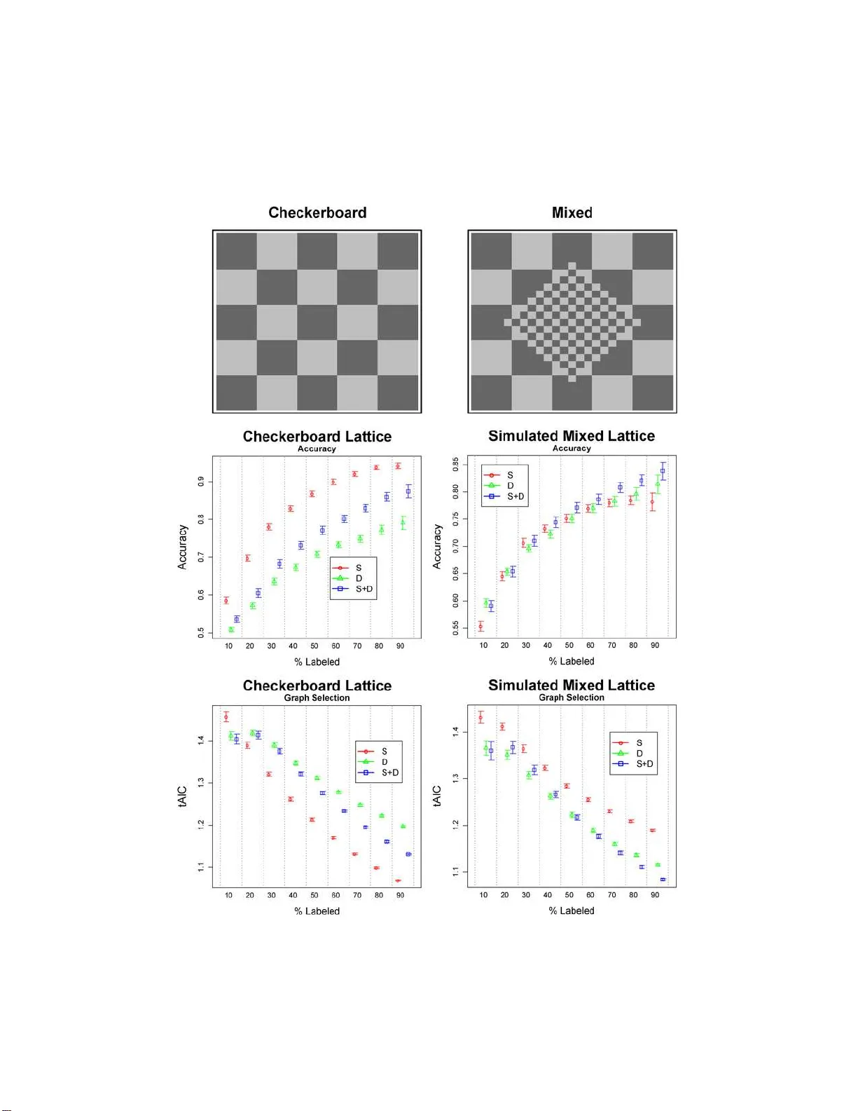
The Annals of Applie d Statistics 2009, V ol. 3, No. 1, 292–318 DOI: 10.1214 /08-A OAS202 c  Institute of Mathematical Statistics , 2 009 ON MUL TI-VIEW LEA RNING WITH ADDITIVE MODELS By Mark Culp, George Michailidis 1 and Kjell Johnso n West Vir g i nia University, University of Michigan and Pfizer Glo b al R ese ar ch & Dev elopment In many scien tific settings data can be naturally partitioned in to v ariable groupings ca lled v iews. Common examples include environ- mental (1st v iew) and genetic informatio n (2nd view) in ecological applications, chemical (1st view) and biolog ical (2n d view) data in drug d isco very . Multi-view data also o ccur in text analysis and p ro- teomics applications where one view consists of a graph with obser- v ations as the vertices and a w eigh t ed measure of pairwise similar- it y b etw een observ ations as the edges. F urt h er, in sev eral of th ese applications the observ ations can be partitioned into tw o sets, one where the resp onse is observed ( labeled) and the other where the re- sp on se is not (unlab eled). The problem for simultaneo usly add ressing view ed data and incorporating un labeled observ ations in training is referred to as multi-view tr ansductive le arning . In this w ork w e in- trod uce and study a comprehensive generalized fixed p oint add itive mod eling framew ork for multi-view transductive learning, where any view is represen ted by a linear smo other. The problem of view se- lection is discussed using a generalized A k aike Information Criterion, whic h pro vid es an approac h for testing the contri bution of eac h v iew. An efficien t implementatio n is pro vided for fi tting t hese models with b oth backfitting and local-scoring type algorithms adjusted to semi- sup ervised graph-based learning. The proposed technique is asses sed on b oth synthetic and real data sets and is sho wn to be comp etitive to state-of-the-art co-training and graph- based techniques. 1. In tro d uction. In man y scien tific applications the a v ailable data come from d iverse d omains wh ic h are r eferred to as views henceforth. Th e views ma y consist of collectio ns of numerical and categ orical v ariables, but also ma y corresp ond to observ ed graph s. The ob jectiv e of this study is to in- tro duce a compr ehensiv e m o deling framew ork for a numerical or catego r - ical resp onse v ariable that is a fu n ction of data from distinct views. As Received January 2008; revised July 2008. 1 Supp orted in part by NIH Grant P4118627. Key wor ds and phr ases. Multi-v iew learning, generalized additiv e mo del, semi- sup ervised learning, smo othing, m o del selection. This is an electronic reprint of the origina l article published b y the Institute of Mathema tical Sta tis tics in The Annals of Applie d S tatistics , 2009, V o l. 3, No. 1, 292–31 8 . This reprint differs from the or ig inal in pagination and typo graphic detail. 1 2 M. CULP , G. MICHA I LIDIS AND K. JOHNSON a motiv ating example, consider a collec tion of do cumen ts b elonging to a particular scien tific domain, for example, pap ers in statistics journals. The a v ailable information ab out the do cumen ts can b e organized in the follo w- ing three views: the corpu s of the do cument s, that is, a collectio n of words in the do cumen ts [ Blum and Mitc hell ( 1998 )]; information describin g the do cuments (e.g., title, author, journal, etc.) [ McCallum et al. ( 2000 )]; and the co-citation net wo rk (graph) [ McCallum et al. ( 20 00 ), Neville and Jensen ( 2005 )]. F or the graph, no des corresp ond to do cument s (observ ations) and edges coun t the n um b er of citations to the same pap ers (pairwise similar- it y). T he goal for this problem is to classify a do cument according to an at- tribute (e.g., w hether a pap er is applied or theoretical) where the attribute is k n o wn (lab eled) for only a subset of the do cuments, with the remainder b eing unkno w n (unlab eled). In this con text, the do cuments m ust b e labeled b y h uman action, whereas the view information can b e obtained in an auto- mated fashion (i.e., the set of lab eled observ ations L is significan tly sm aller than the u nlab eled one; | L | ≪ | U | ). F urther, it is worth noting that the fi rst t wo views can b e stru cturally r epresen ted by a data m atrix with ro ws cor- resp ond ing to ob s erv ations (d o cument s) and columns to v ariables, but the third view is giv en directly in the form of an obser ved graph. Another example of m u lti-view data arises in drug disco v ery app lications. Supp ose that a very large n um b er of charact eristics (e.g., > 1000) has b een collect ed for a library of chemical comp ounds. These c h aracteristics range from high throughp ut screening measuremen ts of comp ound s’ effectiv eness against n umerous biological targets [ Lundb lad ( 2004 ), Hunte r ( 1995 )] to a comp ound’s absorption, distribution, metab olism, excretion and to xic- it y (ADMET) p rop erties [ F o x et al. ( 1959 ), Kansy , Senner and Gub emator ( 2001 )]. F urther, giv en the c hemical structur e of a comp ound, it is n o wada ys fairly easy to computationall y measure p h ysical prop erties of eac h com- p ound [ Leac h and Gillet ( 2003 )]. Giv en data on the resp on s e of a sub set of comp oun ds in a libr ary for a particular target (e.g., whether or not a side-effect is asso ciated with the comp oun d), the goal is to use the data a v ailable in these diverse views (biological, c hemical, ADMET) to predict the resp onse for the remaining mem b ers in th e library . Notice also th at the target status of a p oten tial dru g can b e b oth time consuming and h ard to determine (e.g., side effects in humans ma y tak e man y y ears to app ear), whereas the biologica l and c hemical comp ound c haracteristics can b e ob- tained in a shorter time p erio d (usually days to we eks) and with less effort (hence, | L | ≪ | U | ). Other examples of multi-view prob lems are pr esen t in applications inv olving genomic [ Nabiev a et al. ( 2005 )] and proteomic data [ Y amanishi, V ert an d Kaneh isa ( 2004 )]. As illustrated with these examples, the av ailable data can b e naturally partitioned int o disjoin t data sets, r eferred to as views, th at in some cases can b e r ep resen ted as data matrices, while in other cases come in the form MUL TI- VIEW LEARNING WITH ADDITIV E MOD ELS 3 of graphs. Views comprised of v ariables can differ in the n umb er of v ari- ables, v ariable t yp e (n u m erical, ordinal, nominal), n oise leve l and scale. Graph v iews may differ in the no d e degree distribution, t yp e and distri- bution of edge weigh ts. T raditionally , mo dels for the prediction problem at hand h a ve b een built that include all the v ariables a v ailable, without taking in to consideration the presence of distinct views. F urther, data in the form of an obs erv ed graph w ere ignored completel y . Popular tec h niques for build- ing flexible prediction mo dels include recursive partitioning [ Breiman et al. ( 1984 )], multiv ariate adaptiv e regression splines [ F riedman ( 1991 )], rand om forests [ Breiman ( 2001 )], su pp ort vec tor mac hines [ V apnik ( 1998 )], partial least s q u ares [ Mevik and W ehrens ( 2007 )], etc. Nev ertheless, there are sev- eral situations where incorp orating distinction of views offer a n umb er of adv an tages from a data analysis p oin t of view, including: • View level analysis : In many applications it is of great in terest to dev elop a mo del that pro vides insigh t into the u nderlying relationship among views, p oten tially iden tifying in teractions b et we en them, and also to assess their predictiv e capabilities. The latter can p ro ve particularly useful in problems where colle cting the necessary data for a view may b e r esource d emanding and thus exp ensiv e. • Inc orp or ation of gr aph information : As already discussed, in man y ap- plications some of the av ailable data come in the form of a graph that a v ailable statistical mo d els can not h an d le in a straigh tforward mann er. • Impr oving pr e dictive p erformanc e : Allo wing the a v ailable d ata to b e p ar- titioned in to different views and incorp orating in teractions among them offers the adv an tage of bu ilding more flexible and p oten tially more p o wer- ful mo dels, exhibiting b etter p erformance in terms of prediction accuracy . In this w ork w e introdu ce an additive mo deling framew ork that take s int o consideration th e presence of distinct data views. F ur ther, it incorp orates in a seamless fash ion observed graphs, allo ws for view lev el analysis and on man y o ccasions leads to significan t gains in p er f ormance. The main idea of this framew ork is to repr esen t eac h view by a linear smo other. The d ifficultly is in pr o viding repr esen tativ e m u lti-dimens ional view sm o others on an y data typ e (graphs or n u merical/cate gorical) , while accoun ting for the sp ars e labeling of the resp onse whic h o ccurs in sev eral of the applications u nder consideration ( | L | ≪ | U | ). T o d efi ne a smo other for an observe d graph, we build on recent adv ances in grap h -based transdu c- tiv e learning [ Blum and Mitc hell ( 1998 ), Zhu ( 2007 )]. Sp ecifically , graph - based transductiv e learning addresses th e pr oblem of learning in a setting where the a v ailable data come in the form of a graph (lab eled and unla- b eled observ atio ns corresp ond to vertice s /no des and pairwise asso ciations to edges), where a numerical or categorical v ariable can also b e associated with eac h no de on th e graph. In this con text, Culp and Mic h ailidis ( 2008a ) 4 M. CULP , G. MICHA I LIDIS AND K. JOHNSON note that the adjacency matrix of th e appropriately n ormalized graph leads to a sto c h astic matrix th at resem bles a kernel smo other with a transductiv e form defined on b oth lab eled and unlab eled no d es. In this w ork we d efi ne a tr ansductive smo other in general as a linear smo other defined for a resp onse that h as a missing un lab eled comp onent. In the case of numerical, categorica l or ordinal data views, it is fairly str aigh tforwa rd to extend a classical linear smo other [see, e.g., Hastie and Tibshir ani ( 199 0 )] in to a transductiv e one [ Culp and Mic hailidis ( 2008a )]. Up on obtaining the transdu ctiv e smo other for eac h view, the next challe n ge is in fitting a mo del to a smo other of this form, since the smo other is linear in the resp onse partitioned with a lab eled (observ ed) and u nlab eled (missing or un observ ed ) component. T o address this, w e p rop ose a n o ve l generalized fi xed p oint self-training fr ame- w ork (Section 2 ) that essen tially extends th e classical generalized additive mo del in to the m ulti-view transdu ctiv e setting. Under reasonable conditions on the transd uctiv e smo other, the solution is guarantee d to uniqu ely exist. In addition, the computational iss ues are add r essed using established iterativ e self-training p ro cedures f or b oth th e regression and classification settings [ Culp and Mic hailidis ( 2008a ), Zhu ( 2007 )]. The p rop osed mo deling framew ork treats b oth the v ariable and graph views repr esen ted by the transdu ctive smo others as th e equiv alen t of “v ari- ables” in a generalized additiv e mo del which can sub sequen tly b e fitted b y an extension of the common bac kfitting (lo cal scoring) algorithm to self- training. Due to the lin earity of the solution in the resp onse v ariable, existing mo del selec tion tec hniques can b e readily applied to select im p ortant views. Also, the smo others require estimation of un derlying p arameters, as in the classical case, and we in vesti gate a criterion more appr op r iate for transduc- tiv e smo others defined on views. Th e results indicate that the multi -view mo del using this estimation approac h is quite comp etitiv e with the state-o f - the-art m ulti-view tec h niques discuss ed next. 1.1. R elevant existing multi-view le arning appr o aches. W e p ro vid e n ext a brief exp osition of existing appr oac hes geared to w ard impr o ving accuracy in multi-view learning pr oblems. It is natural to consider the general semi-sup ervised classificatio n p rob- lem as a precursor to the multi-view setting. In semi-sup ervised learnin g a relativ ely small p ercen tage of th e observ ations (cases) con tain lab els. Th e ob jectiv e is to us e the lab eled cases and their relation to the u n lab eled cases to complete the lab eling of the data. Up on lab el completion, the classifier can b e u sed to pr ed ict new cases (indu ctiv e) or must b e retrained/up dated (transductiv e) to incorp orate this inform ation int o the classifier. V arious al- gorithmic solutions a v ailable for this problem in clude self-training [ Abney ( 2004 )], graph r egularizatio n [ W ang and Z hang ( 2006 )], semi-su p ervised SVM [ Chap elle, Sindhw ani and Keerthi ( 2008 )], a n d parametric mo dels MUL TI- VIEW LEARNING WITH ADDITIV E MOD ELS 5 [ Krishnapu ram et al. ( 2005 )]. F or example, in Zhu, Ghahramani and Laffert y ( 2003 ) the authors prop ose a qu adratic energy optimizatio n problem lead- ing to a h armonic estimate for the u n lab eled data with the constrain t that their lab eled estimate retains the original lab els. This appr oac h has seve ral connections with electrical circuits [ Zhu, Ghahramani and Laffert y ( 2003 )], ST-minicut clustering tec h niques [ Blum and Chawla ( 2001 )], sp ectral ker- nel tec hniques [ Joac hims ( 2003 ), Johnson and Zh an g ( 2007 )], an d k ernel smo othing ap p roac hes [ Laffert y and W asserman ( 2007 ), Culp and Mic h ailidis ( 2008 )]. T h e surv ey b y Zhu ( 2007 ) and the b o ok by Chap elle, Sch¨ olk opf and Zien ( 2006 ) highligh t sev eral of these semi-sup ervised approac hes and address b oth theoretical and pr actical issues. In m u lti-view learning Blum and Mitc hell ( 1998 ) develo p ed a co-training pro cedur e for classification problems that is based on the idea that b etter predictiv e mo dels can b e foun d at th e in dividual view lev el, rather than fit- ting a m o del directly on all the a v ailable views. The co-training pro cedure trains a separate classifier for eac h view and then pro ceeds in a self-training fashion by iterativ ely treating the most confid en t unlab eled observ ations as true lab eled ones using the fitted class estimates as the true v alues. After a presp ecified num b er of iterations, co-training pro d uces a classification of ev ery observ ation in th e d ata. A fin al classifier can b e f orm ed through a com bination of the individu al view classifiers, in ord er to pr edict new ob- serv ations un a v ailable during the training ph ase. The intuition b ehind this approac h is that if the r esults of the individu al cla ssifiers arriv e at the same classification for either a lab eled observ ation (kno w n resp onse) or, more im - p ortant ly , an unlab eled observ ation (un kno wn resp onse), and the views are conditionally indep endent, then it is highly lik ely that the deriv ed classifi- cation is correct [ Blum and Mitc hell ( 1998 ), Abn ey ( 2002 )]. Another set of pro cedures are based on a trans d uctiv e graph-based learn- ing setting [ Joac hims ( 2003 ), Zhu ( 2007 ), Culp and Michai lidis ( 2008 )], where the und erlying graph is either observ ed d irectly or constr u cted from the d ata matrix. In this setting, eac h v iew can b e captured by a graph with its cor- resp ond ing adjacency matrix, and the views are in tegrated by adding their adjacency m atrices. F or example, the Sp ectral Graph T ransdu cer (SGT) treats the r esulting graph as an energy net w ork, wh ere the lab eled obser- v ations are p ositiv e or negativ e sources and the ob jectiv e is to determine an optimal ener gy estimate for the u n lab eled resp onses [ Joac hims ( 2003 )]. An app roac h th at s h ares some of the SGT’s charac teristics is the Sequen tial Predictions Algorithm (SP A), wh ic h forms the final graph by usin g graph theoretic op erations suc h as u nions and int ersections [ Culp and Mic h ailidis ( 2008 )]. This pro cedu re emplo ys a lo cal kernel smo othing algorithm with a regularized extrapolation p enalt y that sh rinks the estimates of u nlab eled no des farther a wa y from lab eled ones to w ard the class prior d istribution. It can b e seen that su c h graph-based pr o cedures can naturally in corp orate 6 M. CULP , G. MICHA I LIDIS AND K. JOHNSON m u ltiple views. Ho w ever, views comprised of n um erical v ariables must fi rst b e con ve rted in to graphs, whic h ma y not b e th e most effec tiv e wa y of rep- resen ting the data. F urther, high p erformance classifiers su c h as supp ort v ector machines or random f orests cannot b e u s ed in th is setting. The p rop osed mod eling framework shares some f eatures with existing co- training and graph based app roac hes. How ev er, by build in g a smo other for eac h view and then com bining them through a generalized add itiv e mo d el, the pr op osed approac h offers useful to ols suc h as view level analysis and incorp oration of graph terms, together with p erformance improv emen ts. The remainder of the p ap er is organized as follo ws: In Section 2 we in tr o duce the mo deling framew ork and address estimati on and mo d el s electio n issu es. Section 3 illus trates the m o del on a n u m b er of real and sim ulated data s ets. Some concluding remarks are drawn in S ection 4 . 2. Mo deling framewo rk for m ulti-view data. F or the problem at hand, let Y denote th e resp onse v ariable of length n = | L ∪ U | , p artitioned into the set L of lab eled observ ations and U of unlab eled ones (sp ecifically Y U is m issing with | U | ≥ 0), that is, Y = [ Y ′ L Y ′ U ] ′ . T he a v ailable predictors can b e p artitioned into q distinct views, w here views m a y consist of v ariables, observ ed graphs or b oth. Views comprised of numerical, nominal or ordinal v ariables are represen ted by data matrices X ℓ of size n × p ℓ . It is assumed that a particular v ariable can only b e pr esen t in one view. Eac h individu al data matrix can b e partitioned ro w-wise in to t wo disjoin t lab eled and unla- b eled sets: X ℓ = [ X ′ L ℓ X ′ U ℓ ] ′ . Views can also corresp ond to observ ed graphs, G ℓ = ( N ℓ , E ℓ ), with N ℓ = L ∪ U denoting the no de set and E ℓ the edge set. The similarit y we igh ted n × n adjacency matrix A ℓ for observ ed graph G ℓ can also b e partitioned in the follo wing wa y: A ℓ =  A ℓ LL A ℓ LU A ℓ U L A ℓ U U  , with A ℓ LL , A ℓ U L , A ℓ U U represent ing edges b et ween lab eled n o des, b et ween lab eled and unlab eled n o des and b et ween unlab eled no des, resp ective ly . As noted ab o ve, the resp onse v ariable is partitioned in to a lab eled and unlab eled comp onen t, w hic h ind uces the corresp ond ing partitions to X and G , resp ectiv ely . The p rop osed mo deling framew ork accommo dates multiple views, as well as their interact ions, as follo ws: η = α + X i f j i ( X j i ) + X i f ℓ i ( G ℓ i ) (2.1) + X i,i ′ f j i ,j i ′ ( X j i , X j i ′ ) + X i,i ′ f ℓ i ,ℓ i ′ ( G ℓ i , G ℓ i ′ ) , where η = g ( µ ) den otes the link fu nction of the r esp onse Y = [ Y ′ L , Y ′ U ] ′ for whic h Y U is missing, with E ( Y ) = µ , α is an intercept term, { f j i ( · ) } are MUL TI- VIEW LEARNING WITH ADDITIV E MOD ELS 7 smo oth fu nctions defined on the feature space X , and { f ℓ i ( · ) } are s m o oth functions defined on the n o des of G [ Culp and Mic h ailidis ( 2008 a ), Z h u ( 2005 )]. The main difficulty with ( 2.1 ) stems from the transdu ctiv e n ature of the mo del, due to the presence of the missing resp onse v ector Y U . T o fit ( 2.1 ), w e prop ose next a tw o stage optimization framew ork referred to as gener alize d fixe d p oint self- tr aining . F or this approac h, we must first defin e th e tr aining r esp onse as Y Y U = [ Y ′ L , Y ′ U ] ′ with g ( Y U ) ∈ R | U | an arbitrary initializatio n. The training resp onse is then emplo y ed in t w o stages, eac h discussed in detail next to obtain an estimate ˆ Y = [ ˆ Y ′ L , ˆ Y ′ U ] ′ = g − 1 ( ˆ η ) . In th e first stage, the training resp onse Y Y U is employ ed to determine an estimate for η = α + P f i b y solving min f =[ f ′ 1 ,...,f ′ p ] ′ L ( Y Y U , g − 1 ( η )) + J ( f ) , (2.2) where L ( y , f ) is a loss function th at increases as the deviance from y and f increases, and J ( f ) is an approp r iate p enalt y term on f . The k ey issue is that of existence and u niqueness of the r esulting estimate ˆ η ( Y U ) as a fun c- tion of Y U . F rom this p ersp ectiv e, it can b e seen that the p osited p roblem is a “sup ervised” one with resp ect to resp onse Y Y U and data X , G . As a result, there are a n umb er of w ell-kno wn approac hes that lead to a uniqu e solu- tion includ ing SVMs, logistic regression, add itiv e mo dels, neur al nets, etc. [ Hastie, Tibshir ani and F riedm an ( 200 1 )]. Up on completing th e fir st stage an estimate ˆ Y Y U = g − 1 ( ˆ η ( Y U )) is obtained for th e entire resp onse v ector Y as a fu nction of Y U . The second stage deals with the problem of optimally determining an appropriate v alue of Y U necessary for training purp oses. It can b e c hosen as the solution to the follo win g optimization problem: min Y U ( g ( Y U ) − ˆ η U ( Y U )) ′ ( g ( Y U ) − ˆ η U ( Y U )) , (2.3) that is, the d eviance b et ween g ( Y U ) and ˆ η U ( Y U ) is m in imized. A moment of r eflection sho ws that the optimal Y U corresp onds to a fixed p oin t. Exis- tence and u niqueness of the fi xed p oin t ˆ Y U = g − 1 ( ˆ η U ( ˆ Y U )) are a ke y issue [ Kakutani ( 1941 )]. In sev eral cases the solution can b e obtained in a direct manner, give n the form of ˆ η ( · ). Ho w ever, in other circumstances the fixed p oint solution must b e appro xim ated. One wa y to app ro ximate is u sing Newton’s m etho d w h ose k th up date step is giv en by ˆ Y ( k +1) U = ˆ Y ( k ) U − ( I − ∇ g − 1 ( ˆ η U ( Y U )) | Y U = ˆ Y ( k ) U ) − 1 ( ˆ Y ( k ) U − g − 1 ( ˆ η U ( ˆ Y ( k ) U ))) . A key assu mption is that the maxim u m eigen v alue of the gradien t ∇ g − 1 ( ˆ η U ( · )) is less than on e, which renders the corresp onding map a contrac tion, thus guaran teeing the existence of a fi x ed p oint . By th e deriv ativ e c h ain ru le, 8 M. CULP , G. MICHA I LIDIS AND K. JOHNSON this approac h requires the gradien t of ˆ η U ( ˆ Y ( k ) U ) for eac h k , whic h can b e computationally demanding to obtain. This motiv ates th e follo wing slo wer iterativ e s elf-training algorithm [ Culp and Mic h ailidis ( 2008a )]: 1. Initialize the unlab eled resp on s e v ector, ˆ Y (0) U and get tolerance δ . 2. Iterate until k ˆ η ( k ) U − ˆ η ( k − 1) U k < δ (a) Solve ( 2.2 ) with resp onse Y ˆ Y ( k − 1) U = [ Y ′ L , ˆ Y ( k − 1) ′ U ] ′ and data { X ℓ , G ℓ } to get ˆ η ( k ) . (b) Set ˆ Y ( k ) U = g − 1 ( ˆ η ( k ) U ). Con vergence of this alg orithm provi des an appro xim ation to the fixed p oint defined in ( 2.3 ) by constru ction. Whenever there exists an in itializa tion that results in lo cal con v er gence of the ab o v e pro cedur e, then the fi xed p oint exists and is approximate d by the algorithm. Moreo ver, if the algo- rithm con verges globally in d ep end ent of the initialization, th en th e fixed p oint is un iquely app ro ximated b y the pr o cedure. The global conv ergence dep end s on the sp ecific choic es for { f j ( · ) } [ Culp and Mic h ailidis ( 2008 a )]. W e provi de b elo w the d etails for fitting this pro cedure first for squared error loss and then for logistic loss when { f j ( · ) } are estimated using transductiv e smo others. Before we discuss transductiv e smo others, w e b riefly address the bias and v ariance of an estimate ˆ f r esulting fr om the prop osed fix ed p oint self-training approac h in the regression cont ext. T o b egin, we consider fi r st the sup ervised case with the goal of estimating a function e f L from data ( X L , Y L ), w here the resp onse Y L is cont in u ou s . It is wel l kn o wn that the s u p ervised error of e f L with resp ect to resp onse Y L can b e decomp osed into bias, v ariance and irreducible terms [ Hastie, T ib shirani and F riedman ( 2001 )]. Recall that the semi-sup ervised problem using the fixed p oint self-training m etho d arriv es at an estimate ˆ f = [ ˆ f ′ L , ˆ f ′ U ] ′ with data ( Y ˆ f U , X ). F rom this, the error of estimate ˆ f w ith resp ect to resp onse Y ˆ f U can b e decomp osed as Error( ˆ f ) = σ 2 + Bias( ˆ f L | X ) + V ar( ˆ f L | X ) + Error( ˆ f U ) , where σ 2 is the irr educible err or term, Bias( ˆ f L | X ) and V ar( ˆ f L | X ) are the resp ectiv e bias and v ariance of the lab eled estimate relativ e to the true function conditioned on the fu ll data X , and Error( ˆ f U ) = 0 b y construction. The resulting sup ervised and semi-sup ervised bias and v ariance terms are giv en b y T r aining Bias/V arianc e Sup ervised Error = σ 2 + Bias( e f L | X L ) + V ar( e f L | X L ) Self-training Error = σ 2 + Bias( ˆ f L | X ) + V ar( ˆ f L | X ). MUL TI- VIEW LEARNING WITH ADDITIV E MOD ELS 9 Therefore, the s elf-training approac h allo ws one to determine a lab eled esti- mate, ˆ f L , that balances the b ias/v ariance tradeoff b y emp loying the en tire X information, wher eas the corresp ond ing sup ervised prob lem achiev es a sim- ilar goal by only u s ing the X L information. Naturally , this decomp osition extends in th e presence of graph views. Remark 1. The connection b etw een the t wo s tage op timization ap- proac h and the self-training algorithm rev eals that this framew ork is a semi- sup ervised example of a blo c k relaxatio n algorithm [see the discuss ion in Leeu w ( 1994 )]. 2.1. Fitting the additive mo del in the r e gr e ssion c ontext. F or ease of pre- sen tation, we study the simplest form of ( 2.1 ) u sing the fixed p oin t self- training appr oac h th at com b in es a numerical/ categorical f eature set X and a graph view G for a con tin u ou s resp onse Y L . T he resulting mo del is giv en b y Y = α + f 1 ( X ) + f 2 ( G ) + ε. (2.4) Our strategy in fitting th is mo del is b ased on constructing transd u ctiv e smo others for b oth the X and G views. W e provide next the details of suc h a constru ction and extend it to incorp orate interac tions among these t wo views. The imp lemen tation details are presente d in Section 2.4 . T o fi t th e f unction η = α + f 1 ( X ) + f 2 ( G ) un d er a squared-error loss cri- terion, we must minimize w ith resp ect to f = [ f ′ 1 f ′ 2 ] ′ the follo win g: min f ( Y Y U − η ) ′ ( Y Y U − η ) + 2 X j =1 λ j f ′ j P j f j , (2.5) where P j ’s are p enalt y matrices for eac h v iew, α = ¯ Y Y U , and λ j > 0 the asso- ciated tuning p arameters. F or a graph view we c h o ose P as the com bin atorial Laplacian op erator, that is, P = D − A , wh ere A is the adj acency matrix and D is its ro w-su m diagonal m atrix. F or X d ata views, there are m any c hoices, including generalized additiv e mo dels, sp line-based mo dels, nonp arametric mo dels, etc. [ Hastie and Tib shirani ( 1990 )]. Belo w w e provi de more details on the p enalt y matrix for the graph case (Section 2.1.1 ) and for the feature X d ata case (Section 2.1.2 ). No matter ho w it is obtained, eac h p enalt y matrix emits the follo wing partition: P j =  P LL j P LU j P U L j P U U j  . (2.6) In the ab o ve expression, the submatrix P LL captures asso ciations b et we en lab eled p ortions of the data, wh ile P U L and P LU lab eled to u nlab eled data asso ciations, and finally P U U unlab eled to unlab eled ones. E ac h p enalt y 10 M. CULP , G. MICHA I LIDIS AND K. JOHNSON matrix, P j , is assumed to b e p ositiv e semidefinite, whic h in turn implies that the problem in ( 2.5 ) is join tly con ve x. T herefore, one can s olv e it to obtain th e f ollo wing equations: ˆ f ℓ − S ℓ Y Y U − X j 6 = ℓ ˆ f j ! = ~ 0 for ℓ = 1 , 2 with S ℓ = C ( I + λ ℓ P ℓ ) − 1 , (2.7) where C = ( I − 11 ′ /n ) is a cente ring matrix. Th is is clearly an extension of the Gauss–Seidel algorithm with resp onse Y Y U and sm o others { S ℓ } 2 ℓ =1 :  I S 1 S 2 I   ˆ f 1 ( X ) ˆ f 2 ( G )  =  S 1 Y Y U S 2 Y Y U  . (2.8) The solution of th e Gauss–Seidel algorithm is wel l kn o wn to tak e the form ˆ η ( Y U ) = α + ˆ f 1 ( X ) + ˆ f 2 ( G ) = RY Y U with smo other R indep end en t of Y Y U [ Hastie and Tib shirani ( 1990 )]. Therefore, the first stage in our mo d el fitting strategy results in a linear fitting tec hniqu e, ˆ η ( Y U ) = R Y Y U . F or the fixed p oint step ( 2.3 ), we need to define the class of tr ansductive smo others generated from X , G or b oth as follo ws: A [ · ] = { S : S is an n × n linear smo other matrix constructed from s ou r ce su c h that ρ ( S U U ) < 1 } , where S ∈ A [ · ] emits the partition S =  S LL S LU S U L S U U  , (2.9) and ρ ( · ) denotes the sp ectral radius of the matrix un der consideratio n. The partitions in the transductiv e smo other corresp ond to the partitions in the p enalt y matrix giv en ab o ve, that is, ( 2.6 ). F rom the first optimization prob- lem discus s ed ab ov e, we get that for an y smo other S the unlab eled estimate is giv en b y ˆ η U ( Y U ) = S U L Y L + S U U Y U . The optimization prob lem in ( 2.3 ) subsequently reduces to min Y U (( I − S U U ) Y U − S U L Y L ) ′ (( I − S U U ) Y U − S U L Y L ) , and th erefore, the condition that ρ ( S U U ) ≡ ρ ( ∇ ˆ η U ( · )) < 1 results in ˆ Y U = ( I − S U U ) − 1 S U L Y L as the un ique fi x ed p oint. F rom this, in the case of a regression mo del a closed form solution can b e obtained as  ˆ Y L ˆ Y U  =  S LL + S LU ( I − S U U ) − 1 S U L ( I − S U U ) − 1 S U L  Y L . (2.10) As exp ected, th e resulting p redicted resp onses are linear in the lab eled data Y L , that is, ˆ Y = M L · Y L , with M LL and M U L the resp ectiv e | L | × | L | , | U | × | L | matrices iden tified in parenthesis in the ab o ve expression. MUL TI- VIEW LEARNING WITH ADDITIV E MOD ELS 11 A sp ecial case arises wh en f 1 ( X ) is mo deled by a linear mo d el, that is, f 1 ( X ) = X β . The additiv e mo del in ( 2.4 ) redu ces to the follo wing semi- parametric m o del: Y = X β + f 2 ( G ) + ε, whic h is fit u sing transductive smo others, S 1 = H = X ( X ′ X ) − 1 X ′ and cen- tered symmetric smo other S 2 = S defin ed on G . The goal is to obtain a closed form expression for β and f 2 suc h that ˆ η = X ˆ β + ˆ f 2 . W e first as- sume that the solution un iquely exists for eac h Y U , that is, there exists a unique R with ˆ η ( Y U ) = R Y Y U . No w apply ( 2.8 ) to get that ( X ′ X ) − 1 ˆ β ( Y U ) = X ′ ( Y Y U − ˆ f 2 ( Y U )) and ˆ f 2 ( Y U ) = S ( Y Y U − X ˆ β ( Y U )), whic h yields ˆ β ( Y U ) = ( X ′ ( I − S ) X ) − 1 X ′ ( I − S ) Y Y U and ˆ f 2 ( Y U ) = S ( Y Y U − X ˆ β ( Y U )) . Therefore, th e Gauss–Seidel algorithm obtains the fun ction estimate ˆ η ( Y U ) = ( I − S ) X ˆ β ( Y U ) + S Y Y U ≡ RY Y U . F or the fixed p oin t phase, we assume that ρ ( R U U ) < 1 to get that ˆ Y U = ˆ η U ( ˆ Y U ) = X U ˆ β ( ˆ Y U ) + ˆ f 2 U ( ˆ Y U ). P r ofiling out ˆ f 2 U from ˆ Y U and after some algebra, w e get that ( X ′ ( I − S ) X ) ˆ β = X ′ ( I − S ) Y Y U = X ′ ( I − S )[ e Y + X ˆ β ] − X ′ L ( I − M LL ) X L ˆ β , where M LL = S LL + S LU ( I − S U U ) − 1 S U L and e Y L = [ Y ′ L , e Y ′ U ] ′ with e Y U = ( I − S U U ) − 1 S U L Y L . Solving for the co efficien t yields the follo wing estimate for b oth β and f 2 : ˆ β = ( X ′ L ( I − M LL ) X L ) − 1 X ′ L ( I − M LL ) Y L , (2.11) ˆ f 2 L = M LL ( Y L − X L ˆ β ) and ˆ f 2 U = M U L ( Y L − X L ˆ β ) , (2.12) with M U L = ( I − S U U ) − 1 S U L . This results in ˆ η L = ( I − M LL ) X L ˆ β + M LL Y L , whic h is the natural generalizat ion of the classica l semi-parametric mo d eling result [ Hastie and Tibshir ani ( 1990 )]. 1 In general, one can apply the Gauss–Seidel algorithm directly to a se- quence of sm o others with eigen v alues in ( − 1 , 1]. The algorithm is guarantee d to conv erge to a solution w henev er the smo others are diagonally dominant, or symmetric and p ositiv e semid efi nite. In other words, one can forgo the first optimization pr oblem and apply th e Gauss–Seidel algorithm directly to 1 In the case of the linear mod el without the graph t erm [i.e., f ( X ) = X β or f ( X ) = ψ ( X ) β ], we have that ( 2.11 ) with M LL = 0 results in ˆ β = ˆ β ( ls ) = ( X ′ L X L ) − 1 X ′ L Y L (i.e., th e sup ervised ordinary least squares estimate), which is consistent with Culp and Michai lidis ( 2008a ). 12 M. CULP , G. MICHA I LIDIS AND K. JOHNSON a sequence of sm o others defined on X and G , analogous to the sup ervised setting [ Hastie and Tib shirani ( 1990 )]. F or the second step, the solution to the optimizatio n problem tec hnically exists whenev er th e fi nal matrix R is a transductiv e smo other. Thus, with wel l defin ed sm o others one can alw ays follo w th is appr oac h to obtain ( 2.10 ). 2.1.1. Obtaining tr ansductive smo oth ers f or gr aph views. W e elab orate next on ho w to obtain the smo other matrix S from an observe d graph view G . The graph is repr esen ted b y its weigh ted n × n adjacency m atrix A defin ed ab o ve, with A ( i, j ) ≥ 0. The normalized r igh t sto chastic smo other matrix S is then defined by S = D − 1 A , with D b eing a diagonal matrix con taining the ro w sums (no de d egrees) of A . Notice that the matrices A , D and S all emit the necessary p artition structure giv en in ( 2.9 ). F or example, the w eighte d similarity adjacency matrix A has four blo c ks: the A LL blo c k pro- vides weigh ted links b et wee n lab eled observ ations, the A U L and A LU blo c ks are weig h ted links b etw een lab eled and unlab eled observ ations, and the A U U blo c k is comprised of weig h ted lin ks b et ween unlab eled and unlab eled ob - serv ations. F or the do cument classification example, the we igh ts are defined b y docu m en t similarit y b et ween observ ations in L ∪ U . In the C orollary to Prop osition 2 in Culp and Mic h ailidis ( 2008 a ), we established that ρ ( S U U ) < 1 when ev er A U L × 1 L > ~ 0 and A U U is irreducible (i.e., these assump tions are sufficien t for S ∈ A [ G ]). The condition on A U L is in terpr eted th at eac h un lab eled n o de h as at least one connection to a lab eled no de. In d ata in volvi ng graphs it should b e noted that this condition is difficult to satisfy , esp ecially when the s ize of the lab eled set is small relativ e to that of th e unlab eled s et, as illustrated in Figure 1 . T o account for this, one could start with the observed graph, compute the sh ortest path distance b et ween no des and obtain a new complete graph on eac h component (all no d es are connected to all other no d es within eac h comp onen t), and then, subsequ en tly , “thin ” the obtained graph . Notic e that these additional steps can circumv en t the p roblem by generalizing to ev ery disconnected comp onent must hav e a lab el on it as discussed in Culp and Mic h ailidis ( 2008 a ). The ab o ve sm o other is generally to o simplistic to p erform w ell on real data since there is no tuning parameter λ . One wa y to add ress this is to define the com binatorial Laplacia n as P = D − A and then, s u bsequently , generalize the smo other to S = ( A + λP ) − 1 A or the symmetric smo other S = ( I + λP ) − 1 in ( 2.7 ). Either of these generalizat ions tend to impro v e p erforman ce o v er that of the stochastic sm o other sin ce the p arameter λ can b e estimated based on the resp onse Y L . 2.1.2. Obtaining tr ansductive smo others for fe atur e views. In the case of feature d ata, it is fairly straight forw ard to obtain the transductive smo other MUL TI- VIEW LEARNING WITH ADDITIV E MOD ELS 13 Fig. 1. A cr oss-se ction of an observation gr aph with b oth lab ele d and unl ab ele d vertic es (observat i ons). The lab ele d vert i c es c onsist of either a lar ge dark or light cir cle, and the unlab ele d vertic es c onsist of smal l black cir cles. The inter est in this example is to il lustr ate the affe ct of unlab ele d data on the top olo gy of the gr aph. from th e p enalt y matrix as giv en in ( 2.7 ). How ev er, additional considera- tions are made for the case of constructing transd uctiv e smoother matrices based on k ern el functions, whic h is the approac h primarily us ed in this work. Sp ecifically , one can constru ct a similarit y matrix W , with W ij = K γ ( d ( x i , x j )) with i, j ∈ L ∪ U, (2.13) where d ( · , · ) is a d istance fu nction applied to the v ectors con taining the data for ob s erv ations i and j , and K γ is a ke rnel fu nction. The corresp ond - ing smo other is then given b y S = ( W + λP ) − 1 W , with P the com binatorial Laplacian of W . In the ca se of λ = 1, b y construction, we hav e that S ∈ A [ X ] whenev er W U L × 1 L > ~ 0 and W U U is irreducible as with the graph case. Ho w- ev er, unlike in the graph case, th is condition is t yp ically satisfied in p ractice when using noncompact k ernel fun ctions. On the other hand, p erformance can impro ve b y introd ucing a parameter K and constructing adjacency ma- trix A as the K nearest neighbors d efined by similarit y asso ciations in W (often referred to as a K -NN graph). As a result, the adjacency ma y r e- quire similar mod ifications as ind icated for the observ ed graph to form the smo other S = ( A + λP ) − 1 A (or S = ( I + λP ) − 1 ), w h ere P is now redefined as th e combinatoria l Laplacian op erator defined on the K -NN graph A . 2.1.3. Par ameter estimation. As noted ab ov e, in sev eral instances the prop osed framework requires the estimation of sev eral tunin g p arameters including kernel parameters, nearest neigh b or parameters and Lagrangian parameters. In general, the tuning p arameters can b e broken into t wo groups: within view and b et ween view ones. Th e within view parameters denoted 14 M. CULP , G. MICHA I LIDIS AND K. JOHNSON b y τ are necessary to construct the p enalt y matrix P τ ℓ from either X data sources or graph sour ces [i.e., τ ℓ = ( γ ℓ , k ℓ ) to f orm th e k -NN graph for view ℓ ]. The b et we en view parameters corresp ond to the Lagrangian on the p enalt y matrices for the additiv e mo del and are d en oted as λ = ( λ 1 , . . . , λ q ). Up on completing the w ithin view parameter estimation step, the goal is to obtain a p enalt y matrix, P ℓ , from eac h view ℓ . Th is p r oblem is treated on a view-b y-view basis. F or example, in view 1 sup p ose that it has b een estab- lished th at a ran d om forest learner w orks particularly well and, similarly , for view 2 a neural n et learner is the b est p erf orming one. T o incorp orate this information, w e consider a searc h o ve r the parameter space whic h finds a transductiv e smo other S ℓ that p redicts similarly to the learner. More pre- cisely , let φ L ℓ and φ U ℓ b e th e p redictions of the pro cedure app lied to view ℓ (e.g., a r an d om forest or a n eural net) and define the p enalt y matrix P τ ℓ = D ℓ − W ℓ using th e follo wing criterion: min τ ℓ k φ U ℓ − ( I − S U U ) − 1 S U L Y L k 2 2 with S = D − 1 ℓ W ℓ . (2.14) In other w ords, the goal is to fin d a v alue γ ℓ and k ℓ suc h that the solution in volving smo other S in ( 2.10 ) coincides closely to predictions from learner φ . Notice th at the individu al smo others mimic sp ecifically c hosen learners within eac h v iew, w hic h can resu lt in strong p erf ormance in several data applications [refer to the pharmacology data example in Section 3.3 , wh er e w e observe that the estimate with ( 2.14 ) p erforms qu ite strongly compared to the state-of-the-art co-training algorithms with random forest]. Up on obtaining the appropriate p enalt y matrices, one then must deal with the b et ween view parameter estimation problem for λ in ( 2.5 ). The Lagrangian allo ws one to sim ultaneously accoun t for the sm o other’s con- tribution for eac h view. T o p erf orm this, w e fir s t m ak e use of the fact that the lab eled estimate is linear in Y L ; that is, ˆ Y L = M LL ( λ ) Y L , where M LL ( λ ) = R LL ( λ ) + R LU ( λ )( I − R U U ( λ )) − 1 R U L ( λ ) (the notation is mo di- fied to indicate the dep endance of the smo other matrices on th e parameters). In th is case, we mak e use of the standard GCV criterion adjus ted to trans- ductiv e smo others giv en b y tGCV( M LL ( λ )) = min λ ( Y L − M LL ( λ ) Y L ) ′ ( Y L − M LL ( λ ) Y L ) (1 − tr( M LL ( λ )) /m ) 2 . (2.15) In practice, the tGCV criteria is optimized sim ultaneously for eac h λ j so that adj u stmen ts can b e made b et ween the views. Remark 2. The optimization criterion in ( 2.15 ) can also b e used to es- timate within view parameters wh en a learner is n ot a v ailable. F or example, the parameter k on an observe d graph view could b e estimate d with ( 2.15 ). Ho we v er, in our exp erience, if a learner is a v ailable, then p erformance can impro v e by usage of ( 2.14 ). MUL TI- VIEW LEARNING WITH ADDITIV E MOD ELS 15 2.1.4. Vie w inter action terms. Next w e elab orate on the view interac tion terms pro vided in ( 2.1 ). W e restrict atte ntion to t wo-w a y in teraction terms that pro v e most useful in practice. There are thr ee p ossible t yp es of inter- actions in the presen t setting: an in teraction b etw een t wo views comprised of feature data, f 12 ( X 1 , X 2 ), an in teraction b et ween tw o views comprised of observ ed graphs, f 12 ( G 1 , G 2 ), and, fin ally , an interact ion b et ween a feature and a graph view, f 12 ( X 1 , G 2 ). In this work w e are primarily in terested in the case when the views are mo deled as transductiv e kernel or graph smo others. T he inte raction term can b e defined as a comp osite graph op eration, wh ic h can b e ac hiev ed in v arious w ays. One p ossibilit y is to use the intersect ion, while another the union of the underlyin g t wo graphs. The in tersection b et w een tw o graphs G i ∩ G j with corresp onding weigh ted adjacency matrices W i , W j is defi ned b y a new graph wh ose adj acency matrix is giv en b y [ W ij ]( u, v ) = q W i ( u, v ) W j ( u, v ), while that for their union, W ij = W i + W j 2 . 2 These terms are then pro cessed as add itional smo others in ( 2.8 ). Remark 3. Another approac h for defi n ing inte ractions is giv en in Hastie and Tib shirani ( 1990 ) wh ere the authors emplo y restrictions on the f 12 ( · , · ) term durin g estimation. Extensions of this app roac h to ( 2.1 ) could also b e considered esp ecially for interact ions with nonk ern el based terms (e.g., linear terms). 2.2. Fitting the mo del in classific ation. In classifica tion we assume that the resp onse tak es on b in ary v alues, Y L ∈ { 0 , 1 } . The goa l is to fit a general semi-sup ervised multi-vi ew mo del of the form η = α + f 1 ( X ) + f 2 ( G ) , with η = g ( µ ) , where g is the logit link fun ction. Next we utilize the gener- alized fixed-p oint self-training strategy to ac hieve this ob jecti v e. As previously discussed, one must fi rst obtain the training resp onse as Y Y U = [ Y ′ L , Y ′ U ] ′ , where g ( Y U ) ∈ R | U | . F or the firs t s tep in ( 2.2 ), we optimize for ˆ η in min η L ( Y Y U , g − 1 ( η )) + 2 X j =1 λ j f ′ j P j f j , (2.16) 2 There are other possibilities for defining the union term, how ever, we compute it additively [ Gould ( 1998 )]. It shou ld b e noted that when interaction terms are included in the mo del, care should b e taken to av oid identifiabilit y issues arising from the follo wing situation: f 12 ( G 1 ∪ G 2 ) ≈ f 1 ( G 1 ) + f 2 ( G 2 ) − f 12 ( G 1 ∩ G 2 ). 16 M. CULP , G. MICHA I LIDIS AND K. JOHNSON where the logistic loss function ( L ( y , p ) = − y log( p ) − (1 − y ) log(1 − p ) with p = g − 1 ( f )) is u sed and P j are the ap p ropriate p enalt y matrices for X, G , resp ectiv ely . The solution to this p roblem ˆ η ≡ ˆ η ( Y U ) must satisfy λ i P i ˆ f i − ( Y Y U − g − 1 ( ˆ η )) = ~ 0 . Emplo yin g a T aylo r expansion on g − 1 ab out ˆ η ( k − 1) and setting it to zero, w e get the follo wing s emi-sup ervised extension of the z-scoring algorithm: ˆ f ( k ) i − S ( k − 1) i ( ˆ η ( k − 1) − ˆ f ( k − 1) i ) = S ( k − 1) i z ( k − 1) , where th e smo other is giv en by S ( k − 1) i = C ( W ( k − 1) + λ i P i ) − 1 W ( k − 1) , the score by z ( k − 1) = ˆ η k − 1 − W ( k − 1) − 1 ( Y Y U − g − 1 ( ˆ η ( k − 1) )), and th e v ariance function by W ( k − 1) = ∇ g − 1 ( η ) | η = η ( k − 1) . It is easy to see that the ab o ve for- m u lation reduces to an ap p lication of the Gauss–Seidel algorithm for eac h z ( k ) . Unlik e the regression setting, the smo other for the solution dep ends on Y U , since W dep ends on Y U , and hence, we requir e that there m u st ex- ist a R ( Y U ) s u c h that ˆ η ( Y U ) = R ( Y U ) z ( Y U ). No w, if W is diagonal, then z U ( Y U ) = ˆ η U − W − 1 U U ( Y U − g − 1 ( ˆ η U )). F r om the fixed p oin t step ( 2.3 ), we get that g ( ˆ Y U ) = ˆ η U ( ˆ Y U ) = z U . The iterativ e self-training algorithm discussed ab o ve must b e applied in ord er to obtain this fi xed p oint. The follo w in g prop osition pro vides a s u fficien t condition for the algorithm to conv erge in- dep end en t of its initializatio n (in this case the fixed p oin t must b e unique): Pr oposition 1. Assume that the solution ˆ η = P j ˆ f j exists and satisfies λ j P j ˆ f j − ( ˆ Y Y U − g − 1 ( ˆ η )) = 0 for any Y U such that g ( Y U ) ∈ R | U | . Assume, additional ly, tha t ther e exi sts a ˆ Y U that satisfies the fixe d p oint solution to ( 2.3 ), i.e. g ( ˆ Y U ) = ˆ η U ( ˆ Y U ) . If ρ X j X i 6 = j [( I − S j S i ) − 1 S j ( I − S i )] U U ! < 1 , with S i = ( λ i P i + W ) − 1 W and W = ∇ g − 1 ( η ) | η = ˆ η , then the iter ative self- tr aining metho d c onver ges indep endent of initialization. The condition on the ab o v e matrix is not of m u ch practical use, but, nev erth eless, it provides a general setting for w hic h the solution to ( 2.3 ) uniquely exists. 2.3. Mo del sele ction issue s. Give n the multi- view mod el ( 2.1 ) dev elop ed ab o ve, the next imp ortan t issu e to address is that of mo del selection, esp e- cially in the pr esence of m ultiple views and their int eractions. W e pr esen t MUL TI- VIEW LEARNING WITH ADDITIV E MOD ELS 17 next a criterion for ac hieving this ob jecti v e. T o start, for ease of pr esentati on consider a mo del inv olving a feature d ata view X and a graph view G . In this w ork th e inte rest is in view-nested mo del comparisons; f or example, to assess the significance of view in teraction term compare η = α + f 1 ( X ) + f 2 ( G ) + f 12 ( X, G ) , (2.17) η = α + f 1 ( X ) + f 2 ( G ) . (2.18) An example of suc h a m o del comparison is illus tr ated with the Cora text data (Section 3.2 ). The generalized fixed p oint self training framew ork provides a natural en viron m en t to assess m o del selection in the multi-vi ew setting. F or example, let ˆ η 1 = R 1 z 1 and ˆ η 2 = R 2 z 2 represent t wo mo del estimates. One approac h to compare t w o s m o others is Ak aik e’s Information Criterion (AIC). AIC compares t wo mo dels by p en alizing the loss of the mo del under consideration with the degrees of freedom of the smo other ( tr( M LL j )), where M LL j is linear in z L j for mo del j . Mo dels with low er AIC generally fi t b etter and are less complex than mo dels with larger AICs [ Hastie and Tib shirani ( 1990 ), Hastie, T ib shirani and F riedman ( 2001 )]. The AIC mo del comparison for transductiv e sm o others is form ally give n b y tAIC( M LL j ) = 2 m Loss( M LL j ) + 2(tr( M LL j )) m , (2.19) where the Loss( M LL j ) is the L ( Y L , g − 1 ( M LL j z L )) for some loss fu n ction L (for th is w ork w e use the logistic loss function). The b est mo del is the one corresp ondin g to the smo other that minimizes tAIC. Also, when optimizing tAIC w e preserve the h ierarc hical constrain t, that is, the pr esence of higher lev el interac tion terms require lo wer level terms in th e m o del. 2.4. Implementation issu e s. The prop osed fitting pro cedur es emplo y ei- ther the Gauss–Seidel algorithm directly , or indirectly through th e z-scoring metho d. Ho wev er, for regression it is computationally adv anta geous to em- plo y an iterativ e bac kfitting pro cedur e, as opp osed to solving the Gauss– Seidel equations d irectly [ Hastie and Tib shirani ( 1990 )]. Th e main idea b e- hind bac kfitting is to iterativ ely smo oth eac h fu nction to the partial residu al without that function and subs equ en tly mean cen ter the f u nction. A gener- alizati on to the local scoring algorithm is applicable to the generalized ad- ditiv e mo d el setti ng. C on vergence of b oth algorithms are discuss ed globally for several p ossible smo other c hoices [ Buja, Hastie and Tib s hirani ( 1989 ), Hastie and Tib shirani ( 1990 )]. T he transdu ctiv e lo cal scoring algo rithm is present ed in Algorithm 1 and can b e used to fit all the in teresting mo dels under consid eration; note that iterativ e bac kfitting is a s p ecial case of it. 18 M. CULP , G. MICHA I LIDIS AND K. JOHNSON Algorithm 1 T rans d uctiv e Lo cal Scoring 1: Initialize v ector ˆ Y (0) U of size n , and select a smo other t yp e for eac h view (e.g. kernel, linear, spline, etc.) . In put tolerance δ > 0. 2: for k = 1 , . . . do 3: Apply the local scoring algo rithm in tro duced in Buja, Hastie and Tibshir an i ( 1989 ) with smo other t yp e sp eci- fied and r esp onse Y ˆ Y ( k − 1) U = [ Y ′ L , ˆ Y ( k − 1) ′ U ] ′ to determine th e estimate ˆ η ( k +1) = [ ˆ η ( k +1) ′ L , ˆ η ( k +1) ′ U ] ′ . 4: Up date ˆ Y ( k +1) = g − 1 ( ˆ η ( k +1) ) and h en ce ˆ Y ( k +1) U = g − 1 ( ˆ η ( k +1) U ). 5: Stop if k ˆ η ( k +1) U − ˆ η ( k ) U k < δ . 6: end for The ab o v e algorithm tends to globally con v erge in practice, bu t the rate of con verge n ce dep ends significantly on the choic e of ˆ Y (0) U . Th e follo win g argu- men t provides a fairly conv enien t initializ ation for this pro cedure. Consider the regression problem in ( 2.5 ) with r esp onse Y Y U . Previously , we solv ed for ˆ η ( Y U ) = R Y Y U and obtained the fixed p oin t directly . No w, instead, we apply ( 2.7 ) to get that ˆ f ℓ ( Y U ) = S ℓ ˆ ε ℓ ( Y U ), where ˆ ε ℓ ( Y U ) = Y Y U − ˆ η ( − ℓ ) ( Y U ) is the partial residual, and solve to get that ˆ η U ( Y U ) = S U L ℓ ˆ ε L ℓ + S U U ℓ Y U + ( I − S U U ℓ ) ˆ η ( − ℓ ) U ( Y U ). Inv ok e step ( 2.3 ) s o that ˆ Y U = ˆ η U ( ˆ Y U ) and from this w e get that ˆ Y U = ( I − S U U ℓ ) − 1 S U L ℓ ˆ ε L ℓ + ˆ η ( − ℓ ) U . Placing this in ( 2.7 ) for ˆ Y U can- cels out and yields ˆ f ℓ = M · L ˆ ε L ℓ , w here M LL ℓ and M U L ℓ are the smo others iden tifi ed in ( 2.10 ) for view ℓ . F rom this, one can then apply backfitting di- rectly on cen tered s m o others M LL ℓ with r esp onse Y L to obtain an estimate ˆ Y (0) L . T o obtain th e estimate ˆ Y (0) U , one could pr edict w ith the bac kfitting algorithm using smo others M U L ℓ , resp onse Y L and previous estimates ˆ Y (0) L . The in itializat ion ˆ Y (0) U tends to b e rather close to the solution from the self- training algorithm with cen tered smo others S ℓ and resp onse Y ˆ Y U , and hence, the algorithm conv erges fairly fast. A s im ilar in itializat ion can b e der ived for the more general lo cal scoring version. Remark 4. When either bac k-fitting/lo cal scoring are emplo yed for function estimation one must approxima te the degrees of f reedom used for m easur emen ts s u c h as tGCV and tAIC; for example, a common ap- pro x im ate for the denominator of ( 2.15 ) is (1 − [1 + P ℓ (tr( M ℓ ) − 1)] / | L | ) 2 [ Hastie and Tib shirani ( 1990 )]. 3. Data examples. T o assess the p erformance and usefulness of the pro- p osed mo d el, w e h a ve s elected three div erse d ata examples. In the first ex- MUL TI- VIEW LEARNING WITH ADDITIV E MOD ELS 19 Fig. 2 . T he grid of data given on the l eft has a two-class r esp onse r epr esente d by the light gr ay and dark gr ay p oints. We c onsider c onne cting p oints using squar e neighb orho o ds and diagonal neighb orho o ds, which c orr esp ond to the lattic e (right p anel). ample a syn thetic data set comprised of t w o graph views is examined . In the second example an observed graph is com bin ed with a feature set ob- tained from text data. In the third example we apply our approac h to a pharmaceutical problem. 3.1. Gr aph sele ction with disjoint lattic es. W e consider data from a t wo- dimensional latt ice comprised of 625 n o des on a 25 × 25 grid (refer to Fig- ure 2 ). Th e example consists of t wo separate sim ulated complex r esp onse patterns on the graphs as sho wn in Figure 3 (row 1). F or eac h resp onse configuration, w e allo w for tw o d ifferen t w ays to connect neigh b oring nod es: square and diagonal (refer to Figure 2 ). Let L s b e the adjacency matrix for the squ are neigh b orho o d lattice and L d for the d iagonal neigh b orho o d lattice . T he follo wing mo d el w as considered for eac h resp onse configuration (c hec k erb oard, or mixed): η = α + f s ( L s ) + f d ( L d ) . (3.1) The ob jectiv e wa s to determine wh ic h graphs w ere imp ortant for predicting the resp onse in eac h configuration using classification acc uracy and the tAIC measure. In th e analysis we first sampled 10% of the observ ations in the lattice to b e treated as lab eled no des (case s), wh ile the r emaining 90% w ere tr eated as unlab eled cases. T h e w eight matrix for eac h lattic e confi guration (square, and mixed) was constructed by W ij = K γ ( d sp ( i, j )), with K γ ( d ) = e − d/γ , where d sp ( i, j ) denotes the shortest path from no de i to no d e j on the lattice (note i, j ∈ L ∪ U ). Th e p enalt y matrix for the lattice w as giv en b y P = D − W , with D the diagonal ro w su m matrix of W . In the es- timation of η = α + f ℓ ( L ℓ ) with ℓ ∈ { s, d } the smo others w er e giv en by S ℓ = ( W ℓ + P ℓ ) − 1 W ℓ and the parameter γ ℓ w as estimated using the tGCV criterion. F or the additive mo d el, η = α + P f ℓ , the p enalt y matrix P ℓ , th e k ern el matrix W ℓ and the p arameter vect or λ w er e supp lied to the lo cal 20 M. CULP , G. MICHA I LIDIS AND K. JOHNSON Fig. 3. T he r esp onse c onfigur ations ar e pr esente d in r ow 1. The ac cur acy for e ach r e- sp onse c onfigur ation is gi ven in r ow 2, while the tAIC for e ach r esp onse c onfigur ation is given in r ow 3. S denotes squar e m o del, D denotes diagonal mo del, and S+D denotes additive mo del. MUL TI- VIEW LEARNING WITH ADDITIV E MOD ELS 21 scoring algorithm as in put. Ho wev er, b efore pro ceeding with lo cal scoring, the λ parameters we re estimated sim ultaneously using the tGCV criterion analogous to the approac h d iscussed in Hastie and Tib shirani ( 199 0 ). 3 This pro cess w as rep eated 50 times. Then , the ent ire analysis wa s executed w ith Q % of the data treated as lab eled ( Q = 20 , 30 , . . . , 90). The a ve rage accuracy (second column) and tAIC (third column) for eac h lab eled partition s ize is rep orted in Figure 3 . The accuracy plot for the c h eck erb oard example illustrates that the mo del with squ are neighborh o o ds exhib ited the b est p erformance. I n the graph selection plot the square neigh b orh o o d graph pro vid ed the optimal mo del in terms of smallest tAIC. Therefore, the mo del su ggests that the square neigh b orho o d view fits the d ata we ll, in accordance w ith the un derlying c heck erb oard configur ation. F or the mixed configuration, the additiv e mo del p erformed marginally b etter th an the other configurations. Ho w ev er, as the size of the lab eled data grew, the square and diagonal graphs minimized tAIC. 3.2. T ext analysis. In our next example w e consider 776 do cuments ob- tained from the artificial in tellige nce/mac hine learnin g segmen t of th e cora text data [ McCal lum et al. ( 20 00 )]. The artificial in telligence segmen t con- sists of text d o cument s that address the general topics of machine learnin g, planning, theorem pr o ving, rob otics, exp ert s y s tems and others. The bin ary resp onse is the in dicator that th e text do cu men t is sp ecifically ab out ma- c hine learnin g. T he first view corresp onds to the co-cita tion net work, where the vertic es are the lab eled and unlab eled text d o cuments, and the edges are th e n um b er of times that eac h pairwise obs erv ation agree in citation (co-cit ation). Sp ecifically , the adjacency matrix is constru cted as A ij =  T otal # of do cuments co-cited w ith i, i = j , X I { i and j cite the same do cum en t } , i 6 = j . The second v iew con tains 141 carefully parsed words used in the title of eac h of the text do cum en ts (e.g., le arn , net , the ory , etc.). The text string is a partial matc h where the fir st letters of the word in the title m u st matc h the v ariable; f or example, if the v ariable is net , then the observ ation r epresen ts a count of an y v ariation of net , ne ts , network , etc. The follo wing logistic mo del wa s used : η = α + f 1 ( X title ) + f 2 ( G cite ) + f 12 ( X title , G cite ) . (3.2) 3 T o sp eed- up compu tation, transd uctive b ac kfitting was employ ed with resp onse Y L treated as contin uous for only t he parameter estimation comp onent. T ransductive lo cal scoring wa s used for fi tting the actual mo del in each step. 22 M. CULP , G. MICHA I LIDIS AND K. JOHNSON Fig. 4. (left) The plot pr ovides the aver age ac cur acy over 50 samples fr om applying the multi-viewe d mo del on the c or a text data as the amount of l ab ele d data varies fr om 10% to 90% . (right) The c orr esp onding tAIC plot is pr ovide d. T and C denote the m o dels c onstructe d using the wor d view and the citation view, r esp e ctively. T + C is the main effe cts additive mo del, and T+C+T *C is the ful l mo del including the inter action b etwe en views. T o compute the in teraction term, we employ the intersectio n op eration b y defining W 12 ij = q W 1 ij ∗ A 2 ij , wh er e W 1 is the k ernel matrix on the title view and A 2 is the co-cita tion adjacency matrix. Th e goal is determine the simplest mo del to adequately predict whether a d o cument is classified as addressing the sp ecific topic of mac hine learning in th e artificial in tellige nce net work. As b efore, the p ercent age of labeled cases was v aried fr om 10% to 90%. The a verage accuracy results, based on 50 replications, are sho wn in Figure 4 (left panel) and the tAIC resu lts in Figure 4 (righ t panel). Cosine dis- similarit y wa s u sed to construct the distances b et wee n observ atio ns on the title view and tGCV was us ed to estimate the parameters. T he accuracy results tend to fav or the mo dels with b oth the text and citation informa- tion. Th e tAIC measure in dicates that the additive mod el comprised of the text and citation views without inte raction w as th e minimizer. F rom this result we selec t the mo del η = f 1 ( X title ) + f 2 ( G cite ) as d ominan t and drop the in teraction term b et ween X title and G cite . Next, w e assess the prop osed app roac h against the sp ectral graph trans- ducer (SGT), first u sing the G cite view, and then u sing b oth the X title and G cite views [ Joac hims ( 2003 )]. In Figure 5 , the SGT(X, G) dominates in the 10–30 % configur ations and r emains comp etitiv e for the large r lab eled parti- tions. T he SGT(G), how ev er, is only comp etitiv e in the 10% configur ation. MUL TI- VIEW LEARNING WITH ADDITIV E MOD ELS 23 3.3. Drug disc overy data. W e revisit one of the motiv ating examples for this w ork wh ere the obser v ations corresp ond to comp oun ds wh ic h could p oten tially b ecome d r ugs. The goal is to assess early in the dr ug disco v ery pro cess the p oten tial of a comp ound to cause an adv erse even t (AE) or side-effect. Clearly , a comp ou n d’s AE status is critically imp ortant to its success, and as a result, pharmaceutical companies w ould like to iden tify these comp ounds as early as p ossible in the d iscov ery pro cess. The targeted comp ounds can then b e mo dified in an attempt to reduce the adv erse ev ent status while m ain taining their effectiv eness, or eliminated from follo w-up altoge ther. The set of pr edictors consists of inf orm ation describin g the biolog ical rela- tionship (view 1) b et ween a comp ound and a p articular target and the c hem- ical relationship (view 2) whic h p r o vides descriptors based on the structur e of the comp oun d. In order to obtain the necessary biological in formation, a therap eutically r elev an t concen tration of the drug is applied to the target, and the inhibition of the target’s activit y is measured. This view consists of p 1 = 191 con tin u ous and noisy v ariables, eac h consisting of a carefully c ho- sen target. T he c hemical predictors are represen ted b y a sparse and binary set of descriptors ( p 2 = 151), where eac h descriptor represents a sp ecific sub- structure in the comp oun d. F or the data set un der consideration, there are n = 438 comp oun d s, of wh ic h 92 are kn o wn to b e asso ciated w ith a sp ecific AE ( Y = 1, otherwise Y = 0). Fig. 5. The plot pr ovides the ac cur acy r esults with 95% c onfidenc e b ands fr om applying multi-view mo del with the sp e ctr al gr aph tr ansduc er usi ng the c o-citation view only, and the analo gous plots with b oth the title and c o-citation views. The amount of lab ele d data varies fr om 10% to 90%. 24 M. CULP , G. MICHA I LIDIS AND K. JOHNSON Fig. 6. ( left) The plot pr ovides the aver age ac cur acy over 50 samples fr om applying the multi-view mo del [ r e c al l that r andom for est wer e employe d in ( 2.14 )] on the pharmac olo gy data as the amount of lab ele d data varies fr om 10% to 90% . (right) The c orr esp onding tAIC plot is pr ovide d. B and C denote the mo dels c onstructe d using just the biolo gy view and just the chemistry view, r esp e ctively. B+ C is the main effe cts additive m o del, and B+C+B*C is the ful l mo del including the inter action b etwe en views. The 95% c onfidenc e b ands ar e pr ovi de d to assess the pr e cision of the c ontribution for a p articular mo del. In addition to generating a predictiv e mo d el, scien tists are also in ter- ested in assessing the imp ortance of eac h descriptor set. That is, chemica l fingerprints (data in view 2) are extremely c heap to obtain, only requiring computation time, whereas the b iologic al information tak es more time and money to generate b ecause eac h comp ound n eeds to b e assay ed. Hence, as- sessing the imp ortance of b oth views of information has imp ortan t resour ce implications. T o determine the appropriate m o del for this data, the follo win g logistic m u lti-view mo d el was fitted to th e data: η = α + f 1 ( X Bio ) + f 2 ( X Chem ) + f 12 ( X Bio , X Chem ) . The smo others for eac h term in the ab o ve m o del w ere generated by opti- mizing ( 2.14 ), u sing rand om forests in eac h view. The results are shown in Figure 6 f or b oth accuracy and tAIC. In accuracy , the additiv e mo d el tends to imp ro ve o ver that of the c hemistry view only mo del, b ut the im p ro ve- men t is n ot significan t. F rom the tAIC analysis, the additive mod el w ith b oth views seems u seful for smaller lab eled partitions, b ut as the %-lab eled increases, its utilit y diminishes to that of the c h emistr y view only mo del. This result suggests that the biology view and in teractions inv olving this view are n ot con trib uting significan tly to the p erformance of this mo d el. Next, we wish to assess the pr op osed mo deling approac h compared to other m u lti-view pro cedures. F rom th e abov e analysis, th e c hemistry only MUL TI- VIEW LEARNING WITH ADDITIV E MOD ELS 25 Fig. 7. (left) The plot pr ovides the ac cur acy r esults wi th 95% c onfidenc e b ands fr om applying the mul ti-view mo del with r andom f or est, Co-T r aining wi th RF, the sp e ctr al gr aph tr ansduc er, and the r andom for est wi thout a view distinction on the pharmac olo gy data as the amount of lab ele d data varies fr om 10% to 90% . (right) The plot pr ovides the analo gous r esults for the Kapp a p erformanc e me asur e, which b etter ac c ounts f or unb alanc e d classes. view mo del is all that is necessary , but we use th e biology/c hemistry mo del without interact ion for comparison with other m u lti-view techniques. In ad- dition to th e multi-vie w mo del, a random forest without m aking a view dis- tinction was fi tted to the data [i.e., ran d om forest fit directly to (Bio,Chem)], the co-trai ning pro cedur e discussed in the in tro d uction using random forests as the base learner [ Blum and Mitc hell ( 1998 )] and th e S GT approac h wa s emplo yed on this d ata. T o measure p erformance, w e p artition the data into 50 10–90% lab eled groups , eac h with the remainder treated as unlab eled, and app lied b oth accuracy and k appa measures to th e u nlab eled data. The k appa measure is defined as ( O − E ) / (1 − E ) , wh ere O is the observed agreemen t in the testing confusion matrix and E is the exp ected agreemen t [ Cohen ( 1960 )]. V alues close to 0 represent p o or agreement , while v alues close to 1 rep resen t p erfect agreement. Because k appa compares observ ed agreemen t to exp ected agreemen t, it is helpful for assessing p erformance for unbala n ced data. The m u lti-view mo del w ith r andom forest in ( 2.14 ) and th e co-training pro cedur e are q u ite comp etitiv e in b oth the accuracy and k ap p a measures (refer to Figure 7 ). The results b ased on k app a reve al that co-training is somewhat m ore conserv ativ e than the multi-vie w mod el (i.e., tends to pre- dict several observ ations as not having an AE), and therefore, the m ulti-view mo del exhibits a strong p erform an ce in k appa with a sligh t deterioration in accuracy . The su p ervised random forest ap p lied without view distinction 26 M. CULP , G. MICHA I LIDIS AND K. JOHNSON and the S GT p erf ormed p o orly with resp ect to b oth measures for this data set. 4. Concluding remarks. In this pap er we dev elop ed a mo d eling frame- w ork suitable for analyzing multi-view data. I ts main f eatures are: (i) the generalized fi xed p oin t framework to fit semi-sup ervised additiv e mo dels to b oth observed graph and feature views, (ii) mec hanisms to p erform view selection and incorp orate view interac tions and (iii) data-drive n tuning pa- rameter estimation. The p rop osed f ramew ork and sub sequen t devel opmen ts pro v id e a marked departure from the original co-t raining algo r ithms into a data analysis setting by allo wing view interact ions and selections. A topic of fu tu re stud y is the abilit y to assess v ariable con tribution within and b et we en views. In this setting, the individ u al feature views are constructed from v ariables and, therefore, the con trib ution of a par- ticular view dep ends on that of the underlying v ariables. On the other hand, a v ariable’s con tribu tion may o ccur at the view lev el su c h as in an in teraction. Other interesting issu es of study inv olv e in ference, test- ing and transdu ctiv e co v ariance estimation. Th e p ro cess of pred icting new observ ations (as opp osed to retraining, whic h is the current p ro cess) is also under in vestig ation. Th e difficult y of this pr oblem, often referr ed to as in ductiv e learning, is noted in sev eral r eferences [ Culp and Mic h ailidis ( 2008 ), Kr ishnapur am et al. ( 2005 ), Zh u, Ghahramani and Laffert y ( 20 03 ), W ang an d Zh ang ( 2006 ), Z h u ( 2007 )] and is worth y of its own in vestiga - tion. 5. Pro of of Prop osition 1 . Next we pro vide pr o of for Prop osition 1 . Pr oposition 1. Assume that the solution ˆ η = P j ˆ f j exists and satisfies λ j P j ˆ f j − ( ˆ Y Y U − g − 1 ( ˆ η )) = 0 for any Y U such that g ( Y U ) ∈ R | U | . Assume, additional ly, tha t ther e exi sts a ˆ Y U that satisfies the fixe d p oint solution to ( 2.3 ), that is, g ( ˆ Y U ) = η U ( ˆ Y U ) . If ρ X j X i 6 = j [( I − S j S i ) − 1 S j ( I − S i )] U U ! < 1 , with S i = ( λ i P i + W ) − 1 W and W = ∇ g − 1 ( η ) | η = ˆ η , then the iter ative self- tr aining metho d c onver ges indep endent of initialization. Pr oof. By assump tion, w e h a ve that λ j P j ( ˆ f ( k ) j − ˆ f j ) = ( Y ˆ Y ( k − 1) U − Y ˆ Y U ) − ( g − 1 ( ˆ η ( k ) ) − g − 1 ( ˆ η )) , MUL TI- VIEW LEARNING WITH ADDITIV E MOD ELS 27 where ˆ η = ˆ α + P j ˆ f j and ˆ η ( k ) = ˆ α ( k ) + P j ˆ f ( k ) j . W e also hav e that g − 1 ( ˆ η ( k ) ) = g − 1 ( ˆ η ) + W ( ˆ η ( k ) − ˆ η ) + O (1) n, with W = ∇ g − 1 ( η ) | η = ˆ η . Putting these together, w e get that λ j P j ( ˆ f ( k ) j − ˆ f j ) = ( Y ˆ Y ( k − 1) U − Y ˆ Y U ) − W ( ˆ η ( k ) − ˆ η ) + O (1) , and h ence, ˆ f ( k ) i − ˆ f i = S i " W − 1 ( Y ˆ Y ( k − 1) U − Y ˆ Y U ) − X i 6 = j ( ˆ f ( k ) j − ˆ f j ) # + O (1) , with S i = ( W + λ i P i ) − 1 W . After some algebra and solving for a common term, ( I − S i S j )( ˆ f ( k ) i − ˆ f i ) = S i ( I − S j ) W − 1 ( Y ˆ Y ( k − 1) U − Y ˆ Y U ) + O (1) , i 6 = j. Assume W is a multiple of I and defin e R i = ( I − S i S j ) − 1 S j ( I − S j ), then ˆ f ( k ) U i − ˆ f U i = R U U i ( ˆ η ( k − 1) U − ˆ η U ) + O (1) . F rom this, we can cycle the ab o ve statemen ts with i = 1 , . . . , q for ℓ = 1 , . . . , k to get that ˆ f ( k ) L i − ˆ f L i = R LU i q X j =1 R U U j ! k − 1 ( ˆ η (0) U − ˆ η U ) + O (1) , ˆ f ( k ) U i − ˆ f U i = R U U i q X j =1 R U U j ! k − 1 ( ˆ η (0) U − ˆ η U ) + O (1) . Therefore, if [ P q j =1 R U U j ] k → 0 , then con ve rgence of th e algorithm is guar- an teed. The actual initialization ˆ η (0) is of n o consequen ce, ther efore, th e con verge n ce is ind ep end ent of initializati on.  Ac kn o wledgment s. Th e authors would like to thank the area Editor Mic hael S tein, the AE and thr ee anon ymous referees for their usefu l com- men ts and su ggestions. REFERENCES Abney, S. (2002). Bo otstrapping. In Asso ciation for Computational Li nguistics 360–367. Abney, S. (2004). Un derstanding the Y aro wsky algorithm. Comput. Linguist. 30 365–3 95. MR2087949 Blum, A. and Cha wla, S. (2001). Learning from lab eled and unlab eled d ata using graph mincuts. In International Confer enc e on Machine L e arning 19–26. 28 M. CULP , G. MICHA I LIDIS AND K. JOHNSON Blum, A. and Mitchell, T. (1998). Combining lab eled and u nlab eled d ata with co- training. In Pr o c e e dings of the Eleventh A nnual Confer enc e i n Computational L e arning The ory (Madison, WI, 1998). 92100 (electronic). AC M, N ew Y ork. Breiman, L. (2001). Random forests. Machine L e arning 45 5–32. Breiman, L., Friedm an, J., Olshen, R. and Stone, C. (1984). Classific ation and R e- gr ession T r e es . W adsworth Adv anced Book and Soft ware, Belmon t, CA. Buja, A., Hastie, T. and Tibshirani, R . (1989). Linear smo others and additive mod els. Ann . Statist. 17 543–555 . MR0994249 Chapelle, O., Sch ¨ olk opf, B. and Zien, A., e ds. (2006). Semi- Sup ervise d L e arning . MIT Press , Cam bridge, MA. Av ailable at http://www .kyb.tueb ingen.mpg.de/ssl- book/ . Chapelle, O., Sind hw ani, V. and K eer thi, S. (2008). Op timization techniques for semi-sup ervised supp ort vector mac hin es. J. Machine L e arning R ese ar ch 9 203–23 3. Cohen, J. (1960). A coefficient of agreemen t for n ominal data. Educ ation and Psycholo g- ic al Me asur ement 20 37–46. Culp, M. and Michailidis, G. (2008a). An iterativ e algorithm for extending learners to a semi-sup ervised setting. J. Comput. Gr aph. Stat ist. 17 1–27. Culp, M. and Michailid is, G. (2008b). Graph- based semisup ervised learning. IEEE T r ans. Pattern Analysis and Machine Intel ligenc e 30 174–179. F o x , S ., F arr-Jones, S. , Sopchak, L., Boggs, A., W ang, H., Khour y, R. and Biros, M. (1959). High-throughput screening: Up d ate on p ractices and success. J. Bi om ole c- ular Scr e ening 11 864– 869. Friedman, J. (1991). Multiv ariate adaptive regression splines (with discussion and a rejoinder by th e author). Ann. Statist. 19 1–141. MR1091842 Gould, R. (1998). Gr aph The ory . Benjamin/Cummings, Merlo P ark, CA. MR 1103114 Hastie, T. and T ibshirani, R. (1990). Gener alize d A dditive Mo dels . Mono gr aphs on Statistics and Applie d Pr ob abili ty , V ol. 43. Chapman and Hall, Lon d on. MR1082147 Hastie, T ., Tibshirani, R . and Friedman, J. (2001). The Elements of Statistic al L e arn- ing ( Data Mining, Infer enc e and Pr e diction ). Springer, New Y ork. MR1851606 Hunter, W. (1995). Rational drug design: A multidiciplinary approac h. Mole cular Me d- ic al T o day 1 31–34. Jo achims, T. (2003 ). T ransductive learning v ia sp ectral graph p artitioning. In Interna- tional Confer enc e on Machine L e arning 290–29 7. Johnson, R. and Zhan g, T. (2007). On the effectiveness of th e Laplacian n ormaliza- tion for graph semi-sup erv ised learning. J. Mach. L e arn. R es. 8 1489–1517 ( electronic). MR2332439 Kakut ani, S. (1941). A generaliz ation of Brouw er’s fixed p oint theorem. Duke Math. J. 8 457–459 . MR0004776 Kansy, M., Se nner, F. and Gubema tor, K. (2001). Physicoshemical high throughput screening: Paralle l artificial membrane p ermeation assa y in the description of passive absorption pro cess. J. Me dicinal Chemistry 44 923–930. Krishnapuram, B., Wi lliams, D. , Xue , Y., Har temink, A., Carin, L. and Figueired o, M. ( 2005). On semi-sup ervised clas sification. In A dvanc es in NIPS 721– 728. Laffer ty, J. and W asserman, L. (2007). Statistical analysis of semi-sup ervised regres- sion. In A dvanc es in NIPS 801–8 08. Leach, A. and Gillet, V., eds (2003). An I ntr o duction to Chemoinformatics . Kluw er Academic, London. MUL TI- VIEW LEARNING WITH ADDITIV E MOD ELS 29 De Leeuw, J. (1994). Blo ck relaxation algorithms in statistics. In Information Systems and Data Analysis (H . H. Bo ck, W. Len ski and M. M. Rich ter, eds.) 308–325. Sp ringer, Berlin. Lundblad, R. (2004). Chemic al R e agents for Pr otein Mo dific ation , 3rd ed. CRC Press, Boca Raton, FL. McCallum, A., Nigam , K., Re nnie, J. and S eymore, K. ( 2000). Automating the construction of internet p ortals with machine learning. Information R etrieval J. 3 127– 163. Mevik, B. and Wehrens, R. (2007). The pls pac ka ge: Principal component and partial least squares regression in R . J. Statist. Softwar e 18 1–24. Nabiev a, E., Jim, K., Agar w al, A., Chazelle, B. and Si ngh, M. (2005). Whole- proteome prediction of p rotein function via graph-theoretic analysis of interaction map. Bioinformatics 21 302–310. Neville, J. and Jensen, D. (2005 ). Leveraging relational auto correlation with laten t group mo dels. In Pr o c e e dings of Multi-R elational Data Mi ning 49–55. V apni k, V. (1998 ). Statistic al L e arning The ory . Wiley , New Y ork. MR1641250 W ang, F. and Zhang, C. (2006). Lab el propagation through linear neighborho od s. In International Confer enc e on Machine L e arning 985–99 2. Y amani shi, Y., Ver t, J. and Kanehisa, M. (2004). Protein n etw ork inference from multiple genomic data: A sup erv ised approach. Bioinformatics 20 363–370 . Zhu, X. (2005 ). Semi-sup ervised learning with graphs. T ec hnical rep ort, Carnegie Mellon Univ., Pittsburgh, P A. Zhu, X. (2007). Semi-sup ervised learning literature survey . T ec hn ical rep ort, Computer Sciences, Univ . Wisconsin–Madison. Zhu, X., G hahramani , Z. and Laffer ty, J. (2003 ). Semi-sup erv ised learning using Gaussian fi elds and harmonic functions. In International Confer enc e on Machine L e arn- ing 912–919. M. Culp Dep ar tment of St a tistics P.O. Box 63 30 West Virginia University Morgantown, West Virginia 26 506 USA E-mail: mculp@stat.wvu.edu G. Michailidis Dep ar tment of St a tistics 439 West Hall 1085 South University University of Michigan Ann Arbor, Michigan 48109-110 7 USA E-mail: gmich ail@umich.edu K. Johnson Pfizer Global Research & Development Ann Arbor, Michigan 48105 USA E-mail: Kjell.Johnson@pfizer.com