Shocks and finite-time singularities in Hele-Shaw flow

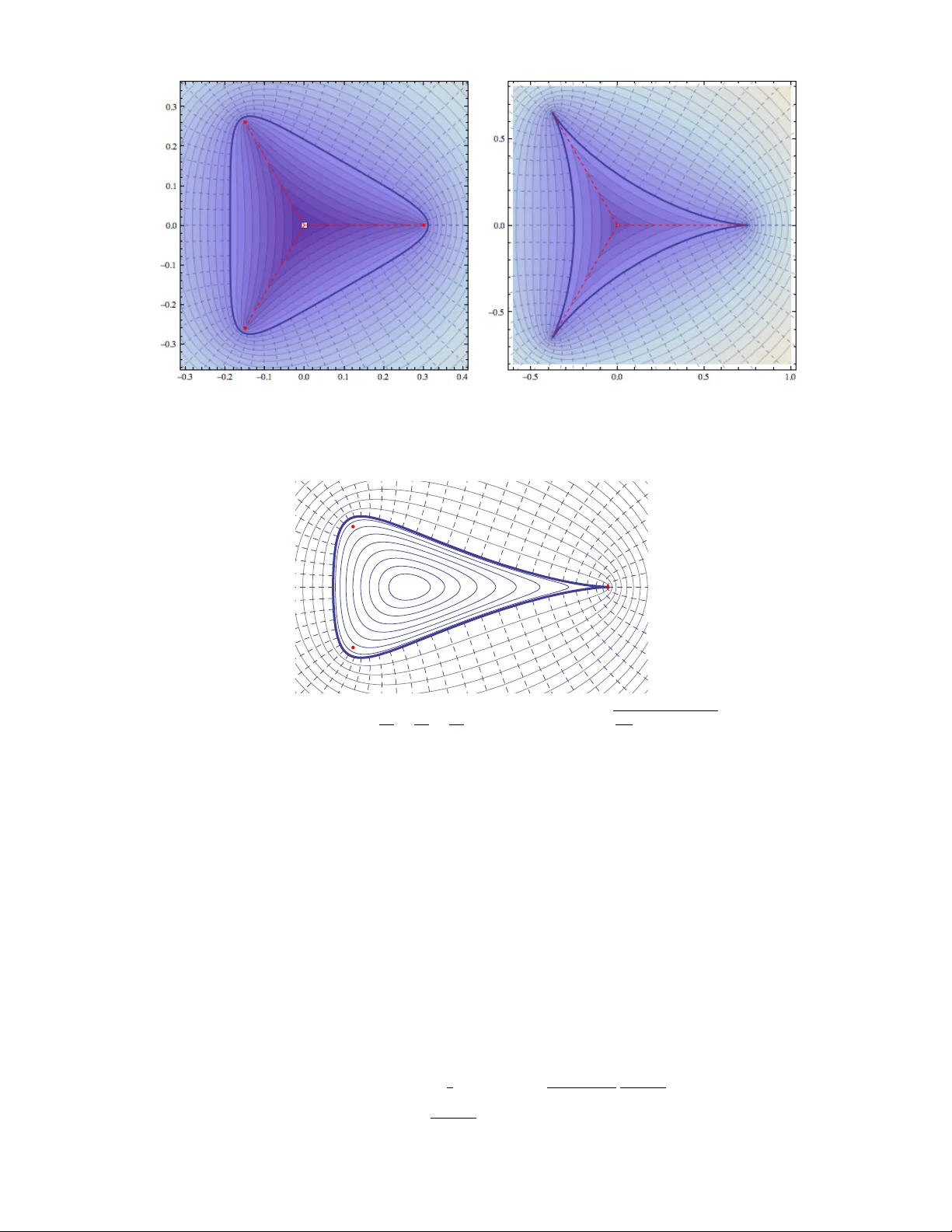
Sho c ks and ﬁnite-time singularities in Hele-Sha w ﬂo w S -Y Lee, 1 R T eo dorescu, 2 and P Wiegmann 3 1 Centr e de r e cher ches math ´ ematiques, University of Montr e al, Montr e al, Canada 2 Center for Nonline ar Studies and T-4, L os A lamos National L ab or atory, L os A lamos, NM 87505, USA 3 The James F r anck and Enric o F ermi Institutes, University of Chicago, 5640 S. El lis A ve, Chic ago IL 60637, USA Hele-Sha w ﬂo w at v anishing surface tension is ill-deﬁned. In ﬁnite time, the ﬂow dev elops cusp- lik e singularities. W e show that the ill-deﬁned problem admits a w eak disp ersive solution when singularities give rise to a graph of sho ck wa ves propagating in the viscous ﬂuid. The graph of sho c ks grows and branches. V elo cit y and pressure jump across the sho ck. W e formulate a few simple physical principles which single out the disp ersive solution and in terpret shocks as lines of decompressed ﬂuid. W e also form ulate the disp ersive weak solution in algebro-geometrical terms as an evolution of the Kric hever-Boutroux complex curve. W e study in detail the most generic (2,3) cusp singularity , whic h give s rise to an elementary branc hing ev ent. This solution is self-similar and expressed in terms of elliptic functions. I. INTR ODUCTION The zero surface tension limit of Hele-Shaw ﬂo ws [1] describes a planar in terface betw een t wo incompressible and immiscible phases propagating with velocity equal to the density of the harmonic measure of the interface. It is a famous problem whose importance go es far b eyond applications to ﬂuid dynamics. Originally formulated b y Henry Darcy in 1856 [2] in relation with groundﬂow of water through porous soil, it describ es a large class of t wo-dimensional growth pro cesses driv en by a harmonic ﬁeld (a.k.a Laplacian growth) and has led to a n umber of imp ortan t developmen ts in mathematics and mathematical physics, from complex analysis to random matrix theory . A compact formulation of the problem is: let γ ( t ) be a simple planar curve – b oundary of a simply-connected domain D . The curv e evolv es in time t according to Darcy Law : v n ( z ) ∼ H ( z ) , z ∈ γ ( t ) . (1) Here v n is the velocity of the curve - an outw ard normal vector from D , and H ( z ) is the normal gradient of a solution of the Diric hlet problem in a ﬂuid domain e D with a source (a sink) at a distan t lo cation (often at inﬁnity in theoretical setup; not shown in Figure 1): H ( z ) = − ∂ n p ( z ) , (2) ∆ p = 0 on ˜ D , p | γ = 0 , p | z →∞ ∼ − log | z | . (3) W e use H ( z ) | d z | for the harmonic measure on the curve γ ( t ). Laplacian growth mo dels [3, 4] are c haracterized b y intricate ﬁnger-like unstable patterns [5] featuring ﬁnite-time singularities [6, 7] in the form of b oundary cusp formation (see e.g. Figures 3, 4). As such the problem is ill-deﬁned: the Darcy la w stops making sense, since v elo cit y and pressure gradient div erge at a critic al time in a critic al p oint , where a cusp-like singularity o ccurs. An imp ortan t feature of Laplacian growth is its in tegrability . In this case, integrabilit y means that, if the initial in terface is an algebraic curve of a given order, it will remain so at all times b efore the critical time. Insigh ts in to in tegrability app eared in early pap ers [8] and then were further developed in more recent studies [9, 10, 11, 12, 13]. Dynamics near a critical p oint (i.e., close to the blow-up time) b elongs to the class of non-linear problems for which an y p erturbation is singular. In this case, v arious regularization schemes t ypically lead to diﬀerent results. This situation is typical in ﬂuid mec hanics and, in fact, similar to singularities appearing in compressible Euler ﬂo ws. There, p erturbing the Euler equations by a diﬀusive mechanism (i.e., b y viscosity), or by a Hamiltonian mec hanism (i.e., b y disp ersion) leads to diﬀerent ph ysics and diﬀeren t ﬂow patterns (as an example compare the dissipative Burgers equation and the Hamiltonian KdV equation, which diﬀer by terms with higher-order deriv ativ es). A traditional lab oratory set-up (called a Hele-Shaw cell after its inv en tor [1]) consists of t w o horizontal plates separated by a narrow gap, initially ﬁlled with a viscous liquid, where inviscid liquid is pump ed in at a constan t rate at the center of the cell, pushing the viscous liquid, aw a y to a sink. Below we will refer to the viscous liquid as ﬂuid , o ccup ying a domain ˜ D . An inviscid liquid o ccupies a complimentary domain D = C \ ˜ D . Both liquids are considered to b e incompressible. The b oundary initially mov es according to the Darcy law (1-3), where p is the pressure of the incompressible viscous ﬂuid. A typical pattern is seen in Figure 1. 2 FIG. 1: (Left) Exp erimen tal pattern in Hele-Sha w cell [14]. The shaded region in b oth pictures is the viscous ﬂuid. (Righ t) Viscous ﬁngering in Hele-Shaw ﬂow. Solid lines are lines of a constan t pressure, dashed lines are stream lines. It seems that the most relev an t mec hanism of taming singularities for exp eriments in Hele-Sha w cell (ev en for a developed pattern as in Figure 1 [14]) is surface tension. Then p in (3) along the in terface is prop ortional to its curv ature. This p erturbation stabilizes gro wing patterns (as seen in Figure 1) but destabilizes their analytical and integrable structure. Also, it is not exp ected that patterns possess universal features if the surface tension is signiﬁcan t. The surface tension eﬀects can be diminished in non-Newtonian ﬂuids where a viscous ﬂuid is substituted by a p olymer solution. In this case, singularities are con trolled by certain visco-ellastic prop erties of the ﬂuid [15]. An interesting mo dern setting consists only of the viscous liquid without the inviscid liquid. In experiments describ ed in [16], a thin lay er of viscous liquid is positioned on a horizontal w etted substrate, with the free b oundary contracting b y some suction mec hanism. [47]The adv an tage of this setting is that the height of the lay er ma y v ary (and indeed do es v ary along the rim [16]), whic h eﬀectiv ely mak es the tw o-dimensional ﬂow compressible. Below we assume such setting that allows the v ariation of compressibilit y , and will keep the name Hele-Shaw ﬂow . Another interesting setting occurs when air propagates through granular media [17]. There, the bo undary is not con trolled b y its curv ature (unlike in ﬂuids with surface tension), but the density of granular media ma y v ary on the b oundary . The traditional approach in studies of Hele-Shaw ﬂow assumes the following order of limits: the densit y of the ﬂuid is set to a constant ﬁrst, while the surface tension is k ept non-zero. Then the limit of surface tension going to zero is tak en, but prov es to b e ill-deﬁned; the solution blows up. This requires a diﬀerent mo del for Laplacian growth, such that the zero surface tension limit (2) is well-deﬁned and do es not lead to a singular solution. Such a view for Laplacian growth is suggested by the setting with a thin la yer on a wetting substrate [16], or propagating air through gran ular media [17] mentioned ab ov e, and also b y the mo del of Diﬀusion-Limited Aggregation (DLA) [18], or iterative conformal maps algorithm [19]. In the latter case, the interface ev olv es by coalescence (aggregation) of Brownian w alkers supplied at a constant rate from a p oint source (inﬁnit y). The probabilit y of aggregation at a giv en p oin t is prop ortional to the harmonic measure of the existent aggregate. In the limit when the area of a particle tends to zero, the problem of aggregation b ecomes iden tical to the ill-deﬁned zero surface tension Hele-Shaw ﬂow. Aggregation contin ues b ey ond this limit, pro ducing notoriously in triguing fractal patterns. In this case, the zero-size limit for particles is a singular p erturbation. Due to a ﬁnite size and irregular shap e of particles, taking the limit of aggregation mo del to the contin uous ﬂuid mechanics eﬀectively leads to a compressible ﬂuid, as in the tw o settings men tioned previously . The geometric regularization suggested by aggregation models is a primary motiv ation of this pap er (and of preced- ing papers [9, 10, 11, 12, 13]). W e will relax conditions that ﬂuids are incompressible and curl-free at a microscale, but will require that liquids are curl-free at a larger scale and then study a singular limit when compressibility v anishes, setting surface tension to zero in the ﬁrst place. 3 Based on this idea, w e will construct a we ak solution of the Hele-Sha w zero-surface tension ﬂow, where: - formation of a cusp singularity is follow ed by expanding sho cks – one dimensional lines through whic h pressure and velocity of the ﬂuid are discontin uous. The densit y of the ﬂuid (which is constant aw a y from the sho c k) b ecomes singular at the sho ck, which can b e interpreted as a deﬁcit of ﬂuid; - sho c k lines form an evolving branching pattern. The geometry of shocks is go verned by transcenden tal equations. FIG. 2: A growing and branching sho c k pattern, with one (left) and tw o (right) generations of branchings. The b old line along the negative x -axis represents a narrow viscous ﬁnger (ﬂuid). At this scale, the viscous ﬁnger is v anishingly narrow. In a subsequent publication, we will describ e connections b etw een weak solutions of the Hele-Shaw problem and a few related mathematical problems. W e will show that: - the lines of discon tinuities (sho cks) corresp ond to accum ulation of zeros of bi-orthogonal p olynomials of large orders; - the shock fron ts are anti-Stok es lines for the isomonodromy problem naturally related to the Whitham a v eraging of solutions of Painlev ´ e equations corresp onding to the integrable mo dels asso ciated with particular types of cusps. Sho c k fronts t ypically form a gro wing, branching tree, as in Figure 2. In this pap er, we pro vide a detailed analysis of the sho c k pattern solution representing the birth of the ﬁrst branching ev ent (Figure 2, ab o ve) of what will b ecome a complicated degree-t wo tree. This solution is self-similar and represents the local branching structure of a dev eloped tree. A comment is in order: t ypically , sho c k wa v es in hydrodynamics are asso ciated with phenomena o ccurring at high Reynolds num bers, due to the inertial term in Euler equations [20]. Here we encoun ter a new situation when a discon tinuous solution o ccurs in a viscous ﬂow where the Reynolds n umber is small and inertia terms are neglected in the Na vier-Stokes equations (see the next section). F or a discontin uit y of this kind, p erhaps “crac k” rather than “sho c k” may b e a b etter name. The pap er consists of three parts: ﬁrst we presen t a few (necessary) known facts ab out singularities in the Hele- Sha w ﬂo w and formulate the problem in terms of inverse b alayage – an imp ortant concept giving insights to the weak solution. Then we formulate the we ak disp ersive solution whic h allows sho c ks, and describ e their hydrodynamics (the Rankine-Hugoniot condition). Next w e formulate the ﬂo w in terms of evolution of a complex curve. This formulation is the most suitable for computations. Finally , we give a detailed analysis of a generic (2,3) – cusp singularity and describ e the elemen tary branc hing ev ent. This particular solution reﬂects the nature of a more general w eak solution. W e start by formulating the diﬀerential and weak forms of zero surface tension Hele-Sha w ﬂo w. 4 I I. DIFFERENTIAL AND WEAK FORMS OF HELE-SHA W FLOW A. Diﬀeren tial form of Hele-Shaw ﬂow A thin lay er of viscous ﬂuid of height b o ccupies an op en domain ˜ D with a smo oth simply-connected b oundary γ ( t ). The ﬂuid is drained from a p oint z = ∞ at a constant rate Q , Figure 1. W e assume a quasi-stationary ﬂo w and therefore neglect the term ∂ v ∂ t in the Na vier-Stokes equation ρ  ∂ v ∂ t + v · ∇ v − ν ∇ 2 v  = −∇ p, where ν is the kinematic viscosit y , and ρ the density of the liquid. W e also as- sume that the Reynolds num b er is small Re = | v | b/ρν → 0, and further neglect the inertial term there. W e obtain ρν ∇ 2 v = ∇ p . F urther assuming a Poisseulle proﬁle for the ﬂow, we replace ∇ 2 z v by its av erage − (12 /b 2 ) v and neglect ( ∇ 2 x + ∇ 2 y ) v , to obtain the Darcy law ρ v = − K ∇ p, (4) where K = b 2 12 ν is called hydr aulic c onductivity . Eviden tly , this approximation is consisten t if the ﬂuid is irrotational ∇ × j = 0 , where j = ρ v , as it is seen from the last formula. If furthermore the densit y is assumed to b e spatially uniform, incompressibility of the ﬂuid ∇ · v = 0 and (4) imply that pressure is harmonic at constant density: ∆ p = 0 . (5) W e will relax the condition of constan t density when deﬁning weak solutions. The ﬂuid is suck ed out at a constant rate Q = H γ j × d l , where γ is oriented counter-clockwise. According to the Darcy la w (4), Q equals − K H γ ∇ p × d l . Therefore, at the drain: p → − Q 2 π K log | z | r ( t ) + O  1 z  as z → ∞ . (6) If the b oundary is smo oth, the pressure on the b oundary is controlled by the surface tension p = σ × curv ature. If surface tension v anishes, the pressure is constant along the b oundary p = 0. Then the pressure is a solution of the Diric hlet problem in the ﬂuid. The time dependent function r ( t ) (kno wn as conformal radius), or capacit y C ( t ) = r ( t ) [21], where R is a cell radius, are important characteristics of the ﬂow. They monotonically grow and ha v e the following hydrodynamic in terpretation [22]: let us compute the p ow er required to drain the ﬂuid: N ( t ) = − R ˜ D ∇ p · j d x d y. Darcy law yields that the pow er is the Dirichlet integral N ( t ) = K R ˜ D ( ∇ p ) 2 d x d y ev aluated as N ( t ) = Q 2 / (2 π K )(log R − log C ( t )) . Then the p ow er is a monotonically decreasing function of time. W e will see that, as a ﬂow approac hes a (2,3)-cusp singularit y and enters into a sho ck regime, capacity increases non-analytically , as a square root of time measured from the critical p oin t. After a singularity , capacit y again increases as a square ro ot of time measured from the critical point. A notable fact is that the co eﬃcient of the square ro ot singularit y changes discon tin uously b efore and after the transition (see Sec. VI D). Ph ysically , it means that the pow er required to pro duce the ﬂo w go es through a discon tinuous c hange ev ery time the sho c k front branc hes, suc h that more p o w er is required than it would b e in the absence of singularity formation [22]. B. W eak form of Hele-Shaw ﬂow Once the ﬂow reaches a cusp singularity , it cannot b e con tinued any longer. The Darcy law written in diﬀerential form loses it meaning at the cusp – harmonic measure there diverges. This situation is typical for diﬀerential equations [23] with conserv ation la ws of hyp erb olic typ e : ∂ t u + ∂ z f ( u ) = 0 . (7) Cauc hy problems with suc h conserv ation laws are ill-p osed, and smo oth initial data evolv e in to singularities devel- oping in ﬁnite time (suc h as sho c ks, vortices, etc.). Darcy equation is of this type. The origin of this phenomenon is that conserv ation equations of hyperb olic t yp e are approximations of well-deﬁned problems. A deformation of these equations b y terms with higher gradients, con trolled by a small parameter ~ , prev ents formation of singularities. If a smo oth solution of a deformed equation u ~ leads to a space-time discon tin uous function u | ~ → 0 as the deformation is remov ed, it is called a w eak solution. A discon tin uit y (a shock fron t) tra v els with a v elo cit y giv en by the Rankine-Hugoniot condition - a weak form of the diﬀerential equation (7) [20, 24]: V = disc f disc u . (8) 5 In most cases, simple physical principles determine a weak solution without actually specifying a regularizing deformation. The b est kno wn example is the Maxwell rule determining the position of sho c k fron t [20], or more generally , the Lax-Oleynik entrop y condition for a visc ous solution of equations with hyperb olic conserv ation laws [23]. Here we assume the same strategy . W e will b e lo oking for a weak solution of the Hele-Shaw problem when the Darcy law is applied ev erywhere in the ﬂuid except a moving, growing and branching graph Γ( t ) ⊂ ˜ D of sho c ks (or crac ks), and where pressure suﬀers a ﬁnite discontin uit y – a weak form of singularit y . Belo w w e form ulate a few simple, natural ph ysical principles whic h will guide us to obtaining a unique weak solution, that we call a disp ersive solution . Sho c ks ma y ha v e diﬀeren t ph ysical meanings depending on the v arious exp erimen tal settings discussed in the In tro duction. In the tw o-liquids setting (traditional Hele-Shaw cell), sho c ks are narrow, extended channels where the in viscid ﬂuid is compressed and carries vorticit y . In the single ﬂuid setting, sho c ks are areas with a deﬁcit of ﬂuid. Sho c ks comm unicate with the bulk of the ﬂuid b y supplying/removing ﬂuid to/from the bulk. Ob viously , for sho c ks to o ccur, the uniform ﬂuid density condition m ust b e relaxed. A diﬀerence b et ween sho c ks and a regular b oundary is that b oth pressure and velocity ha ve steep gradients across a sho ck. Also, the pressure is generally not a constan t along a sho ck line. In the following, we summarize the weak form of Hele-Sha w problem, p ostponing the details to Sec. V. The weak form reads: - the diﬀeren tial Darcy law (4-6) holds ev erywhere, except on the graph of sho c ks, where pressure jumps and the densit y (a constant everywhere else) has a single lay er densit y deﬁcit ρ ( x , t ) = ρ 0 − δ ( x ; Γ) σ ( x , t ) with a line density: σ ( x , t ) > 0 (here δ ( x ; Γ) is the delta-function on a sho c k). Both pressure and line densit y v anish at sho ck’s endp oints e k as p | x − e k | . Sho cks mo v e with velocity whose normal comp onen t V ⊥ is directed tow ards higher pressure regions, and ob eys the Rankine-Hugoniot condition: σ | V ⊥ | = K | disc p | . (9) W e discuss the motiv ation, interpretation and consequences of this solution in sections b elo w. The conditions imp osed are restrictive. They determine a sho ck pattern with a given num b er of legs, up to a ﬁnite n umber of deformation parameters. Shock graphs with one and tw o branching generations are represen ted in Figure 2. I II. FINITE-TIME SINGULARITIES IN HELE-SHA W FLOW The dynamics describ ed by the Darcy la w (1, 2) is ill-deﬁned. This has b een understoo d from diﬀerent angles [5, 8, 25], and can b e seen from a simple argument: let w ( z ) be a conformal univ alent map of the ﬂuid domain ˜ D on to the exterior of the unit circle, | w | > 1; the solution of the exterior Dirichlet problem then reads p ( z ) = − 1 2 log | w ( z ) | , v = 1 2 | w 0 ( z ) | , z ∈ ˜ D . (10) (F rom now on we set K = 1 , Q = π . In these units the area is equal to π × time. In this section we also set ρ = 1). In other words, velocity of a b oundary p oin t is prop ortional to the density of harmonic measure H ( z ) | d z | = | w 0 ( z ) || d z | of that p oin t. As a consequence, a sharp er (more curved) part of the b oundary mov es with a higher velocity than the rest, such that the sharp er part is getting ev en sharp er, until it b ecomes singular. This o ccurs for generic initial data, although a num ber of exceptions are known [26]. W e will demonstrate this mechanism on a simple but represen tative example, but ﬁrst we remind the ma jor feature of the dynamics [8, 25]: let us denote b y t k = − 1 k π Z ˜ D z − k d x d y = 1 2 π i k I γ z − k ¯ z d z , (11) the harmonic momen ts of the ﬂuid, and let the area of the domain D not o ccupied b y ﬂuid b e π t 0 /ρ = Q · t. Parameters { t k } are called deformation p ar ameters . It follows from the Darcy law that [8] ˙ t k = 0 . (12) Let us write the in verse (time-dep enden t) map as z ( w ) = rw + X k ≥ 1 u k w − k , | w | ≥ 1 , (13) 6 where the co eﬃcient r , chosen to b e real positive is the conformal radius (6). According to a standard formula of complex analysis, the co eﬃcien ts of the inv erse map determine the area of the domain D , which we denote by π t , through the ar e a formula [21] t = r 2 − X k> 0 k | u k | 2 . (14) Let us consider a simple example of a domain D whose shap e is giv en by a symmetric h yp otrochoid - an algebraic curv e with a three-fold symmetry suc h that all harmonic moments v anish t k = 0, except for the third one t 3 (see Figure 3): z ( w ) = rw + u w 2 . (15) The ratio b et ween the square of conformal radius r and u can b e expressed through t 3 , as u = 3 ¯ t 3 r 2 . Then the area form ula reads t = r 2 − 2(3 | t 3 | ) 2 r 4 . Clearly , this p olynomial in r 2 reac hes the maximum t c = r 2 c / 2 at r c = 1 / (6 | t 3 | ), and cannot increase further. At this moment, the hypotro c hoid dev elops three sim ultaneous cusp-lik e singularities, Figure 3. The mechanism of the evolution to ward a critical p oin t is: a critical p oint of the in verse map z 0 ( w c ) = 0 is lo cated outside of the ﬂuid at w c = (2 u/r ) 1 / 2 = ( r ( t ) /r c ) 1 / 2 < 1 and mov es in time to wards the b oundary . A t a critical time, the critical p oint reac hes the b oundary , at w = 1. In the critical regime, when the critical p oin t of the conformal map is already close to the b oundary z ( w ) | w = e iφ − 3 2 r c = x ( φ ) + i y ( φ ), the b oundary is lo cally approximated by a r e al de gener ate el liptic curve : X ( φ ) := 2 3 x r c ≈ e ( t ) − φ 2 , Y ( φ ) := 4 y r c ≈ 2 φ 3 − 3 e ( t ) φ, (16) Y 2 = − 4 ( X − e ( t ))  X + e ( t ) 2  2 , e ( t ) = − 4 3 (1 − r r c ) = − 2 3  1 − t t c  1 / 2 . (17) A t the critical p oint t = t c , the curve degenerates further to a (2,3) cusp: Y 2 ∼ X 3 . (18) Close to the critical p oin t, the conformal radius dep ends on time in a singular manner as r /r c − 1 ≈ − 1 2 (1 − t/t c ) 1 / 2 , so that the time dep endence of p o wer b ecomes non-analytic: N − N c ≈ − 1 2 (1 − t/t c ) 1 / 2 . Once the (2,3) singularity occurs, the shap e of the pre-cusp ﬁnger is given b y the elliptic curve (17). Up to a scaling of co ordinates and time the curve is univ ersal - it do es not dep end on details of the original domain: Y ( X , t ) =  1 − t t c  3 / 4 Y X (1 − t t c ) 1 / 2 ! . (19) Self-similarit y is preserved after the ﬂow passes through the critical p oin t, t > t c . This simple analysis has a straightforw ard generalization for all cases where a ﬁnite subset of { t k } k> 0 is non- v anishing. At least for this class of initial conditions, the ﬂow leads to cusp-like ﬁnite-time singularities. F or purp oses of analysis of singularities it is suﬃcient to consider only this set of domains. Of course, the class of initial conditions whic h leads to singularities is m uch wider. W e do not attempt to classify it here. W e only mention that domains with a ﬁnite num ber of non-zero exterior harmonic moments b elong to the class of gener alize d quadr atur e domains. F or generic prop erties of generalized quadrature domains, see e.g., [27]. A. The ﬁrst classiﬁcation of singularities The fact that for rather general initial data, the boundary ev olv es to a cusp-like singularit y had been noticed already in the earlier pap ers [25, 28] where the mo del of Laplacian Growth was originally formulated. F urther developmen ts are found in [5, 6], and [3, 7, 29, 30, 31, 32]. F or the most generic initial conditions, a cusp (2,3) o ccurs. Higher-order cusps and corner-like singularities require sp ecial initial conditions. In [11], it was argued that, if a complement of a ﬂuid domain D is a generalized quadrature domain, then cusps of the t yp e (2 , 2 l + 1) : y 2 ∼ x 2 l +1 are p ossible, and that in the critical regime a ﬁnger dev eloping into these cusps is 7 FIG. 3: Symmetric hypotro choid (15) ev olving under Darcy la w (left) reac hes the (2,3)-cusp singularities (right), when all three critical p oin ts (red dots) hit the b oundary at the same time. The shaded contour lines are the equi-pressure lines. The dashed lines are the stream lines. The red dashed lines are branc h cuts - a skeleton . FIG. 4: Deformed hypertro choid z ( w ) = r w + A r 2 r + A r w + r 2 w 2 with A r = r − 4 r 3 − q 3 r 2 5 − 8 r 4 + 16 r 6 , where one critical p oin t giv es rise to a (2,3) singularit y while t wo other critical p oin ts remain in the domain D . Closed lines inside the critical b oundary sho w the pre-critical ev olution. describ ed by a r e al de gener ate hyp er el liptic curve Y 2 = − 4( X − e ( t )) l Y i =1 ( X − d i ( t )) 2 . (20) This means that a real ov al of the curve - a set where b oth X and Y are real - is a graph of the ﬁnger ( x, y ) = ( X , Y ). The double ro ots d i ( double p oints ) are all lo cated in the ﬂuid domain and simple critical p oints e and −∞ are lo cated outside of the ﬂuid. The condition that no critical p oints are found in the ﬂuid, necessarily means that the exterior critical points coincide, giving double p oints, such that the complex curve is degenerate. A cusp of type (2 , 2 l + 1) o ccurs when the branc h p oin t (real ro ot e ) merges with l double p oints. F or reference, we give explicit form ulas for the generic hyperelliptic curv e (20) following the Hele-Shaw evolution [11]. The curve dep ends on l deformation parameters { t 2 k +1 } , k = 1 , . . . , l (not to b e confused with the harmonic momen ts t k ), and it is uniformized by the formulas X = e ( t ) − φ 2 , Y = P l +1 n =1 ( n + 1 2 ) t 2 n +1 P n − 1 k =0 (2 n − 1)!! (2 n − 2 k − 1)!! ( − e ( t )) k 2 k k ! φ 2 n − 2 k − 1 , (21) t 1 + P l +1 k =1 (2 k +1)!! 2 k k ! t 2 k +1 ( − e ( t )) k = 0 . (22) 8 Here t 1 is a time b efore the cusp singularity , t 1 ∼ t − t c . In [29] it has b een argued that dynamics can b e con tinued through a cusp of the t yp e (2 , 4 k + 1) for the price of an app earance of an unstable p oint when a b oundary touc hes itself. Another stable solution w as found in [13] when the ﬂuid undergo es a genus tr ansition : it b ecomes multiply connected. Ho wev er, in the case of the most generic cusp (2,3) and its descendants (2 , 4 k − 1) , k > 0, no smo oth solutions are p ossible. This situation is the sub ject of this pap er. IV. ALGEBR O-GEOMETRIC FORMULA TION OF HELE-SHA W PROBLEM A. Real algebraic curv e W e brieﬂy review some elemen ts of the algebro-geometric description of the Hele-Sha w ﬂow. It is based on the notion of real complex curv e. A b oundary of an algebraic domain (the only case we consider) is described b y an equation f ( z , ¯ z ) = 0, where f ( z , ¯ z ) = P nm a mn z n ¯ z m is a polynomial. It is pro v ed to b e conv enien t to consider a Riemann surface or real algebraic curve deﬁned b y the equation f ( z , ˜ z ) = f ( ˜ z , z ) = 0, where ˜ z and z are tw o complex v ariables. F or example, a curv e for a symmetric hypotro choid (3) is f ( z , ˜ z ) = ( z ˜ z ) 2 − 4 r c ( z 3 + ˜ z 3 ) + 4( r 2 c − r 2 4 )(1 + r 2 2 r 2 c )( z ˜ z ) − 4 r 2 ( r 2 c − r 2 3 ) [33]. Among man y solutions of the equation f ( z , ˜ z ) = 0 with resp ect to ˜ z (sheets of a curv e), there is one ˜ z = S ( z ) (a ph ysical sheet) which describ es a b oundary where ˜ z = ¯ z , S ( z ) = ¯ z , z ∈ γ . (23) It follows from Darcy law that the time deriv ativ e of function S ( z ) is holomorphic in the ﬂuid. On the b oundary and in the ﬂuid domain e D a complex velocity v = v x − i v y is obtained by 2 v = ∂ t ¯ z = ∂ t S ( z ). Ev erywhere in the ﬂuid the velocity is holomorphic. In terms of the function S the Darcy law reads: 2 v ( z , t ) = ∂ t S ( z , t ) , (24) ∂ t S ( z , t ) =2i ∂ z φ ( z , t ) , (25) where φ ( z , t ) = ψ ( z , t ) + i p ( z , t ) (26) is the potential of the ﬂo w, whose imaginary part is the usual scalar pressure p , and the real part is the stream function ψ . Wherev er pressure is harmonic, the p oten tial is an analytic function. As we hav e said, to study lo cal b eha vior of an isolated cusp, it is suﬃcient to consider domains with a ﬁnite set of non-zero harmonic moments (11). In this case the function S has a multiple p ole at inﬁnity . It is represented by a truncated Laurent series with resp ect to a drain at inﬁnity and an arbitrary regular p oint, say z = 0, outside of the ﬂuid: S ( z ) = S + ( z ) + S − ( z ) , S − ( z ) = tz − 1 + ∞ X k> 1 v k z − k , (27) where we set the p ositiv e part to b e a p olynomial: S + ( z ) = X k> 0 k t k z k − 1 . (28) It enco des information ab out the moments of the exterior [34] and from (24) it do es not evolv e in time (12): ˙ S + ( z , t ) = 0 . (29) P arameters of the ﬂow – time t and deformation parameters t k – can b e seen as residues of the diﬀerential z − k S ( z )d z at z = ∞ (a drain). Befor e a critic al time , complex velocity of the ﬂuid is holomorphic everywhere in the ﬂuid domain. In this case, the negative part of the function S ( z ) is an analytic contin uation of ¯ z to the ﬂuid domain: S − | z ∈ ˜ D = 1 2 π i I γ ¯ ζ d ζ z − ζ = 1 π Z D d 2 ζ z − ζ . (30) 9 In this case, S ( z ) is called a Sch w arz function [35]. All singularities of S − ( z ) are branch p oints lo cated outside of the ﬂuid domain. A generating function – integral of the meromorphic diﬀerential dΩ = S ( z )d z from a p oint of the b oundary of the ﬂuid z γ to a p oint of the ﬂuid Ω( z ) = Z z z γ S ( z 0 )d z 0 , (31) is a conv enien t wa y to describ e Hele-Sha w ﬂo ws. F or example, the b oundary of the ﬂuid giv en b y (23) is a solution of the equation | z | 2 = 2 Re Ω( z ) . (32) A graph of −| z | 2 + 2 Re Ω( z ) close to a critical p oint is plotted in Figure 5. FIG. 5: The plot of −| z | 2 + 2Re R S ( z )d z b efore a critical time (left) and at a critical time (righ t). The heigh t diﬀerence has b een blown-up by scaling the v ertical axis and b y applying arctan. In a critical regime, i.e., close to a cusp, it is conv enient to describ e the b oundary in Cartesian co ordinates Y = 1 2i ( z − S ( z )) and X = 1 2 ( z + S ( z )), and treat Y as a function of X . In these co ordinates [11] Darcy law (24) reads: ∂ t Y ( X , t ) = − ∂ X φ ( X, t ) . (33) This follows from an imp ortant prop ert y of the Darcy law (24): the form d ω = S d z + 2i φ d t is closed. Therefore, the Darcy law is inv ariant under canonical transformations ( z , S ) → ( X , Y ) : d ω = − 2i Y d X + 2i φ d t , up to an exact form. In a critical regime, it is also con venien t to choose a critical p oint as origin and to redeﬁne time t → t 1 ∼ t − t c and deformation parameters as t 2 k +1 = 1 2(2 k +1) res ∞ ( − X ) − k − 1 / 2 Y d X . Then, in the case of a (2 , 2 l + 1) - cusp, a h yp erelliptic curve (20) is a Laurent series with resp ect to the lo cal parameter at inﬁnit y X 1 / 2 : Y ( X ) = Y + ( X ) + Y − ( X ) , (34) Y + ( X ) = P l +1 k =0 ( k + 1 2 ) t 2 k +1 ( − X ) k − 1 / 2 , (35) φ ( X ) = − ( − X ) 1 / 2 + C 12 ( − X ) − 1 / 2 + φ − ( X ) , (36) where Y − and φ − consist of further negativ e p o wers in X 1 / 2 . Here, C is the capacity of a ﬁnger – relative to the capacit y at a critical time (capacit y for a compact set is deﬁned just below (6)). Darcy law then states that the p ositiv e part is conserved: ˙ Y + ( X ) = 0 . (37) Eqs. (20) giv e solutions of the Darcy law written in the form (33) under assumption (35). The parameter φ in (21) (treated as a function of X ) is the complex p otential of the ﬂow at the p oint z = X + i Y ( X ). 10 B. Sk eleton and inv erse b alayage If the num ber of non-zero harmonic moments is ﬁnite, the function S ( z ) (27) has only a ﬁnite-order multiple p ole at inﬁnity and branch p oin ts in the ﬁnite part of the complex plane. Before a critical p oin t forms, all singularities are mo ving branch p oints lo cated outside of the ﬂuid. Their dynamics enco de the entire ﬂow. In this case, there is a unique, special wa y to dra w branc h cuts. They can be dra wn as a (possibly m ulti-comp onen t) curv ed graph Σ( t ) such that the jump of the diﬀerential − idΩ = − i S d z , b eing canonically (counterclockwise) orien ted along the curve through ev ery branch cut, will b e real and p ositive: − i disc S ( z , t )d z = 2 σ k ( z , t ) | d z | > 0 , z ∈ Σ k ( t ) , (38) where k lab els branc hes of the graph. Here the diﬀeren tial is tak en along the cut and | d z | is an elemen t of an arc-length along a cut. The canonical orientation (imp ortant for all signs in formulas b elow) is depicted in Figure 6. If S is treated as a complex vector, then (38) reads disc S = 2 σ k n . (39) up down disc Ω = R Γ S ( z ) dz Γ disc S = S (up) − S (down) = 2i σ ` = i | disc S | disc S = i n n ` V ⊥ V || FIG. 6: In the left panel, we sho w the three p ossible stages of evolution: i) when a branch point is outside the ﬂuid, ii) when a ﬁnger forms a cusp (a branch p oin t is on the b oundary), and iii) when a sho c k develops after a cusp (branch p oin ts are inside the ﬂuid). Canonical orientation of the contour (dashed line Γ) deﬁne how the discontin uities are taken. In the right panel, w e show the normal velocity of the sho ck by the thick arrows and the ﬂow of ﬂuid around the sho ck by dashed arrows. The arro ws illustrate that v orticity carried by a shock is comp ensated by the circulation of the ﬂuid around the sho c k. This fact is equiv alen t with the following analytical contin uation of S − ( z ) (30) to the domain D : S − ( z ) = ρ 0 π Z D d 2 ζ z − ζ = X k Z Σ k σ k ( ζ ) z − ζ | d ζ | , (40) with | d ζ | the arclength measure. In other w ords, S − ( z ) is the electric ﬁeld produced b y a single lay er of c harges σ k distributed along a graph Σ. An imp ortant theorem on generalized quadrature domains [36] tells that σ exists and is unique. The curved and generally multi-component graph Σ, conﬁned in the domain D , is called skeleton or mother-b o dy [36]. Line densities of the skeleton depend on time only through time dep endence of the branch points. If a branch p oin t e ( t ) is simple (which we assume), the line densit y σ ( z , t ) v anishes at the branch p oin t by a semicir cle law as σ ( z , t ) ∼ p | z − e ( t ) | . (41) In the case of the hypotro c hoid (15), the graph consists of three curved lines connecting the branc h p oints. They are dra wn as in Figure 3. In the case of symmetric h yp otro c hoid (15), the branc h cuts are three straight seg- men ts, connecting the branch p oints e ( t ) = 3 2 r c ( r ( t ) /r c ) 4 / 3 × (1 , e ± i 2 π / 3 ), with line densities at the branch p oin ts 11 4(2 / 3) 1 / 2 r c (1 − r 2 /r 2 c )( r c /r ) 2 / 3 [ p | z − e ( t ) | + (4 / 3)( r c /r ) 4 / 3 | z | /r c p | z − e ( t ) | ] (where z is measured from a p osition of a cusp). The ma jor prop erty of generalized quadrature domains (actually serving as deﬁnition) [27] is: area av eraging of an integrable analytic function f ( z ) ov er any domain B is reduced to counting of singularities of the function S ( z ) 1 π R B f ( z )d 2 z = 1 2 π i H ∂ B f ( z ) S ( z )d z . This follows from the represen tation (40): 1 π R B f ( z ) ρ d x d y = 1 2 π i H ∂ B f ( z ) S ( z )d z = R { Σ }∩ B σ ( z ) f ( z ) | d z | . (42) If the domain B do es not contain mo ving singularities or the drain, then the av erage sta ys constant in Hele-Shaw ﬂo w. Conv ersely , if the domain B con tains mo ving singularities, or a drain, the av erage dep ends on time. The procedure of sw eeping a domain B into a line graph { Σ } ∩ B with a line densit y σ is known as (in v erse) b alayage [36]. A Newton p oten tial created by uniformly distributed mass outside of the ﬂuid, measured inside the ﬂuid, in ˜ D , will b e the same as the Newton p oten tial created by the (non-uniform) line densities σ . The bala yage pro cedure allows the following insightful interpretation of Hele-Shaw ﬂow. The “skeleton” – moving branc h cuts – ma y b e considered as time-dep enden t sources of the viscous ﬂuid. In this interpretation, the ﬂuid has no boundary , only time-dependent line sources. An extended ﬂuid occupies all the plane except the sources and mo ves with velocity v = (1 / 2) ∂ t S . The pressure of the extended ﬂuid is deﬁned by v = −∇ p . The original b oundary can then b e restored (if necessary) as a r e al oval of the complex curve - a planar curve where S ( z ) = ¯ z , or (equiv alen tly) a zero-level set of the pressure p = 0. Darcy Law (24, 25) connecting velocity and a complex p otential then applies b oth inside and outside the ﬂuid. In this in terpretation, the entire ﬂo w is encoded b y the motion of the sk eleton, or rather by the motion of end p oin ts of the skeleton. V elo city , pressure and stream function generally hav e ﬁnite discon tinuities across the skeleton. Also, pressure ma y not b e constan t along the sides of the skeleton, while velocity is not normal to the skeleton. A singularit y o ccurs when a gro wing skeleton in tersects the b oundary of the ﬂuid. In the next section, w e form ulate the weak solution of the Hele-Sha w ﬂo w and derive equations for the moving sho c k graph. The same equations are applied for a moving skeleton. Vice-v ersa, an ev olution through a cusp singularity will b e “contin uous” only if sho cks are go verned b y the same law as the sk eleton. V. WEAK SOLUTIONS OF HELE-SHA W PROBLEM A. W eak form of Darcy law: the Rankine-Hugoniot and admissibility conditions No w w e assume that after a singularit y has occurred, pressure is a harmonic function ev erywhere except on a mo ving sho c k graph Γ( t ) ⊂ ˜ D located in the ﬂuid domain, where pressure and stream function hav e ﬁnite discon tin uities. Then so do es the r.h.s. in (25). The function S ( z ) = S + ( z ) + S − ( z ) that w e deﬁned b efore the cusp o ccurs c hanges its prop ert y and is no longer a Sc hw arz function. In particular, it exhibits a discon tinuit y in S − ( z ) along the sho c k (in addition to the skeleton) suc h that: − i disc S ( z , t )d z = 2 σ k ( z , t ) | d z | > 0 , z ∈ Γ k ( t ) . (43) W e keep the same notations for line densities along sho c ks as lines densities along a skeleton (38). W e also assume that sho cks that app ear in the p ost-critical regime do not aﬀect the ﬂuid far aw ay from the critical p oin t. W e require that the lines densities σ k are r e al and p ositive , as for a skeleton (Sec. IV B). This is the ma jor condition. W e illustrate its meaning b elow. Therefore, after the critical time, S ( z ) develops branch cuts in the ﬂuid domain ˜ D in addition to the branch cuts in D . W e write: S − ( z ) = ρ 0 π Z D d 2 ζ z − ζ + X k Z Γ k σ k ( ζ ) z − ζ | d ζ | = Z Σ ∪ Γ σ k ( ζ ) z − ζ | d ζ | , z ∈ ˜ D . (44) With an assumed orientation as in Figure 6, we can in terpret (44) as a deﬁcit of the ﬂuid densit y: ρ = ρ 0 − δ ( z ; Γ) σ ( z ). A commen t is in order. Before a critical time, the function S ( z , t ) in (43) w as analytic in a vicinity of the ﬂuid b oundary , and therefore was a Sch w arz function of that b oundary . Not so anymore after a critical p oint. It jumps at branc h cuts that protrude from a sk eleton. F or the same reason, a domain D (complement to the ﬂuid domain which includes sho cks) is not a a generalized quadrature domain any longer. 12 Let us integrate (25) ov er a closed lo op ∂ B bounding a domain B drawn an ywhere in the ﬂuid. If the loop does not cross a sho c k, w e obtain 1 2 d d t Im I ∂ B S ( z )d z = − Z B ( ∇ · j ) d 2 z = I ∂ B j × dl = I d ψ , (45) 1 2 d d t Re I ∂ B S ( z )d z = Z B ( ∇ × j ) d 2 z = I ∂ B j · dl = I d p, (46) where ∇ × j = ∂ y j x − ∂ x j y is the vorticit y ﬁeld, and ∇ · j = ∂ x j x + ∂ y j y is the divergence of velocity ﬁeld (2 ¯ ∂ j = ∇ · j + i ∇ × j ), and j = ρ v . The ﬁrst tw o equalities in each line of (45, 46) are iden tities, the last is one is the Darcy equation. Let us now consider the integral H ∂ B S ( z )d z ov er a lo op which do es intersect a sho c k graph at one or t wo p oin ts. This in tegral measures the density of the p ortion of a shock surrounded b y the lo op and under (43) sta ys purely imaginary at all times. W e conclude that d d t Re I S ( z )d z = 0 . (47) Letting the contour now shrink to an inﬁnitesimal lo op, we obtain the diﬀerential form of (47) as: d d t Re [disc S d z ] Γ = 0 . (48) The total time deriv ativ e in (48) has tw o contributions: one from the time evolution of the function S ( z ), the other from the motion of sho c ks. W e denote the velocity of the sho ck front (normal to the instantaneous curves Γ), by V ⊥ , directed along the vector n as in Figure 6. Then the total time deriv ativ e (48) b ecomes Re [disc ˙ S d z + ∇ k (disc S · V ⊥ ) | d z | ] Γ = 0 , (49) where ∇ k represen ts the deriv ative along the direction tangent to the front along the vector ` as in Figure 6. F or the ﬁrst term, we use a kinematic identit y Re [disc ˙ S d z ] = 2disc v k | d z | , v alid on b oth sides of the sho ck. F rom the reality of the jump (43) it follows that the second term in (49) is purely real, and equals 2 ∇ k ( σ V ⊥ ) | d z | . T ogether, it yields to the condition ∇ k J ⊥ + disc j k = 0 , J ⊥ = σ V ⊥ , j k = ρ 0 v k . (50) The ﬁrst term in this equation represen ts the transp ort of mass due to motion of the sho ck (normal to the sho ck itself ), while the second is the vorticit y of the surrounding ﬂuid ﬂow. They comp ensate each other. This condition, deriv ed solely from the requirement that σ is real, suggests to interpret a sho ck as a single lay er of positive v ortices. Then σ is the (smo oth part of ) densit y of vortices. The core of the v ortex is of the order of ~ 1 / 2 – the width of the sho c k. Then the reality condition for σ means a zer o-vorticity condition for the ﬂuid. Using Darcy law we replace the ﬂuid velocity in (50) by −∇ k p , and in tegrate (50) along the cut. W e obtain the Rankine-Hugoniot condition σ V ⊥ = (disc p ) n . (51) (the constan t of in tegration is ﬁxed from the assumption that b oth the line densit y and discon tinuit y of pressure v anish at endp oin ts of the cut). The fact that σ > 0 is p ositiv e means that a sho ck mo ves to ward the direction of larger pressure. F urthermore, calculating the discontin uities on b oth sides of the Darcy law and using (43) we obtain ˙ σ = − disc ∇ k ψ . (52) This formula has the following in terpretation. Let us assume the sho c k ﬁlled with some material (say , an in viscid ﬂuid in the Hele-Sha w cell), of line density σ . Then the contin uit y condition ˙ σ + ∇ k ( σ V k ) = 0, tells that this material is moving along the sho ck with v elo cit y V k . Com bining this with (52) and integrating along the sho c k, we obtain a coun terpart of (50): div ergency of the sliding current along a sho c k equals the discontin uity of current of ﬂuid normal to the sho ck (see Figure 6): ∇ k J k − disc j ⊥ = 0 , J k = σ V k , j ⊥ = ρ 0 v ⊥ . (53) 13 In tegrating this formula along a sho c k giv es a counterpart of the Rankine-Hugoniot condition: σ V k = (disc ψ ) ` . (54) A t an end p oint of the sho ck e ( t ), the total velocity of the sho ck matc hes the v elo cit y of the branch p oin t: ˙ e ( t ) =  V ⊥ + V k  | z = e ( t ) . (55) W e notice that (at least close to the endp oin t), the stream of mass is directed tow ards the branch p oin t. The Rankine-Hugoniot conditions (51, 54), inequality (43) and the diﬀerential form of the Darcy equation (25) com bined give the weak forms of the Darcy law. The same conditions hold for a sk eleton before and after critical time. After a critical time, shocks can be considered as contin uation of growth of a skeleton inside the ﬂuid. F rom this p oin t of view, skeleton and sho c ks together form a graph whic h grows under the same law. As we will see b elo w, the b oundary is singled out as a p osition of the ﬁrst branc hing even t. F ollowing branc hing ev ents already o ccur in the ﬂuid as branching sho c ks. Summing up: three conditions σ V ⊥ = (disc p ) n , ˙ σ = − disc ∇ k ψ , σ > 0 , (56) together with the diﬀerential Darcy law outside of the sho ck’s graph constitute the we ak form of Dar cy law . W e note that this weak solution only applies to algebr aic solutions unlike the con v entional Hele-Shaw problem. Though condition (56) tells one ho w the sho c ks and domains ev olve in the next momen t, the determination of the driving force—pressure—is not given by the simple Dirichlet problem as in the conv en tional Hele-Shaw problem. T o obtain pressure one needs to know S ( z ), which contains a ﬁnite num b er of branch cuts and p oles. If the function S ( z ) is algebraic at some momen t in time, integrabilit y of the problem guarantees that it will remain so at all times. B. Algebro-geometrical formulation of the w eak solution Ha ving real complex curve in mind (not only its real ov al) has prov ed to b e useful for studying a Hele-Sha w ﬂo w and is necessary to understand its w eak solutions. A Hele-Shaw ﬂow of an algebraic domain is then understo od as the evolution of a meromorphic diﬀeren tial dΩ = S ( z )d z . The prop erties describ ed ab o ve can be cast as algebro- geometrical prop erties of an algebraic curve: 1. the complex curve is real; 2. the condition that all densities are real yields Re I dΩ = 0 , for all cycles in the ﬂuid; (57) 3. sho c ks form a graph determined by the condition Re disc Ω = 0 , (58) and the admissibility condition 4; 4. the condition that all densities are p ositive yields that Re Ω is incr e asing a wa y from the cut; 5. the meromorphic diﬀerential dΩ has multiple p oles at inﬁnity , the residues at inﬁnity of the diﬀeren tial z − k dΩ are the deformation parameters (11), and time is the residue of the diﬀerential dΩ at inﬁnity . The graph (58) consists of curved lines, sometimes called anti-Stokes lines. Condition 3 selects admissible anti-Stok es lines. Complex curv es ob eying condition 2 are called Krichev er-Boutroux curv es. Evolution of a curve ob eying the Kric hever-Boutroux condition through a change of genus had already app eared in studies of Whitham av eraging in in tegrable systems by Krichev er [37]. Similar condition has b een introduced by Da vid in the theory of 2D quantum gra vity [38], and recently was recognized in studies of distribution of zeros in orthogonal p olynomials by Bertola and Mo [39]. Neither appearance is a coincidence. Semiclassical asymptotes of orthogonal p olynomials and Whitham gen us changing transition are ultimately related to the Hele-Shaw ﬂow. According to prop ert y 3, the real part of the gener ating function Ω( z ) = R z z γ S ( ζ )d ζ , where z γ is a chosen p oin t on the b oundary , is a single-v alued function. The integral of the diﬀeren tial o ver a cycle in volving a drain is H dΩ = 2i t . 14 Being cast in this form the prop erties of the curv e fully and uniquely determine a smo oth Hele-Shaw solution before a singularity is reached, and a weak disp ersiv e solution afterwards. As we ha v e discussed, the b oundary of the ﬂuid (b efore it reaches a singularity) is a degenerate curv e. A singularit y o ccurs when a branch p oin t meets a double p oin t on a b oundary , forming a triple (or higher order) p oint, so the curve further degenerates, while the b oundary of the real o v al forms a cusp. Bey ond this time, the triply-degenerate point splits into three regular branch p oints, so that the curve b ecomes non-degenerate. In other words, going through a singularit y , the curve changes genus. This pro cess is illustrated in Figure 7. In a critical regime (i.e., close to a cusp-singularity), a complex curv e lo cally is h yp erelliptic Y 2 = R 2 l +1 ( X ) (21) and Ω( X ) = − i Z X −∞ Y d X , (59) where −∞ is a distan t p oint on a skeleton (negativ e real axis). In this case Im Ω on b oth sides of the cut has opp osite signs, while Re Ω is zero on the cut. F or hyperelliptic c urv es, conditions 3 and 4 are form ulated in terms of level lines of the ﬁeld of the p otential Re Ω: Re Ω( X ) > 0 , X → Γ; (60) Re Ω( X ) | Γ = 0 . (61) Sho c ks and skeleton are zero lev el lines of the potential Re Ω, suc h that the p oten tial sta ys p ositive in the neigh borho o d. Then the line density of sho cks and the mass deﬁcit accumulated b y a sho c k b etw een tw o p oints X 1 and X 2 are: σ ( X ) = | Y ( X ) | Γ , (62) Z X 2 X 1 σ | d X | = | Im Ω( X ) |    X 2 X 1 . (63) In the next section. we show ho w these tw o conditions uniquely determine the evolution of the elliptic curve through the critical time. VI. BEYOND THE (2,3)-CUSP SINGULARITY: SELF-SIMILAR WEAK SOLUTION Here w e give a detailed analysis of the generic (2,3)- cusp singularit y and illustrate the nature of w eak solution. The computations b elow describ e the evolution of a unique elliptic Krichev er-Boutroux curve. W e emphasize that part of this analysis app eared in the pap ers [38, 40, 41], whic h is devoted to Whitham a veraging of the triply-truncated solution of Painlev ´ e I equation. In this section we again set ρ 0 = 1. W e study the evolution of the elliptic curve (16-19) Y 2 = − 4 ( X − e ( t ))  X + e ( t ) 2  2 , (64) through the critical p oint where e ( t ) | t =0 = 0. It is in order to remind how complex co ordinates X and Y are related to a coordinate z = x + i y of the ﬂuid. It is z /r c = X + i Y ( X ). On the b oundary of the ﬂuid X and Y are real and they coincide with Cartesian co ordinates ( x, y ) of the ﬂuid. Elsewhere X is complex. The co ordinate of the ﬂuid is given by the map X → z . The map cov ers the physical plane twice, as shown in Figure 8, so one must choose a ph ysical branch of the map. Under this map a p oint in the ﬂuid z is in one-to-one corresp ondence with a p oint on the X -plane, except on the ﬂuid b oundary . There, tw o p oin ts z and ¯ z corresp ond to the same X . As it follows from (16) X and Y ( X ) ha ve diﬀeren t scaling X ∼ x/r c , Y ∼ ( x/r c ) 3 / 2 . Therefore at x  r c i.e., at the critical regime where appro ximation of the ﬁnger by the elliptic curve make sense, Y ( X )  X and therefore z ≈ X . Having this fact in mind b elo w w e express the ﬂow in the X -plane. There the b oundary of the ﬂuid – a narrow ﬁnger - is represented by its skeleton – a cut on the negative axis Im X = 0 , Re X < e = e 3 , as in Figure 7. A. Elliptic curve – genus transition Figure 7 illustrates the genus transition of the curve and hydrodynamics of sho c ks. Before the critical time, tw o branc h p oints coincide in the ﬂuid. There, pressure and velocity are smo oth. The branch p oint e 3 is the tip of the 15 FIG. 7: The equi-pressure lines and the ﬂo w (dashed) lines b efore the critical time (left), and after the critical time (right). Pressure of ﬂuid gets larger as the shade gets darker. The b oundary of the ﬂuid is a very narrow ﬁnger y 2 ∼ x 3 around the sk eleton line (the thick line on the real axis) and it is not depicted. The red dots are the branch p oin ts, e 1 , 2 , 3 . Real e 3 is the tip of the ﬁnger. Before the critical time e 2 = e 1 is the double p oin t (larger red dot in left ﬁgure). The thick lines (right panel) connecting the branch p oin ts are the sho cks. They emanate with the angle 2 π / 3 and diverge at their ends by a slightly large angle 0 . 0918498 π + 2 π 3 . In the ﬁgure on the right, the orange and green dashed lines that emanate from the branch p oin ts are not-admissible level lines of Re Ω. The ﬂuid ﬂows to the lighter region, tow ard low pressure. Sho c ks mov e tow ard the darker region (higher pressure). ﬁnger. A t the critical time, the tip meets the double point. After the critical time, the double point splits into t wo branch points. They are the endp oints of the sho c ks. The tip of the ﬁnger e 3 retreats. Fluid go es to wards lo wer pressure (ligh ter regions), creating a deﬁcit on sho cks where ﬂuid decompresses. Sho c ks mov e in the opp osite direction, tow ards higher pressure (darker regions). W e write the curve as: Y 2 = − (4 X 3 − g 2 ( t ) X − g 3 ( t )) = − 4( X − e 3 ( t ))( X − e 2 ( t ))( X − e 1 ( t )) . (65) where e 3 ( t ) , e 2 ( t ) , e 1 ( t ) are time-dep enden t branch p oints. One ro ot, say e 3 , can alwa ys b e chosen to b e real. The other t wo are complex conjugated e 2 = ¯ e 1 . The co eﬃcient in fron t of X 2 do es not depend on time and can be remov ed b y translation, such that e 3 + e 2 + e 1 = 0. The positive part of the curve is ± Y + = 2i X 3 / 2 − i g 2 4 X − 1 / 2 . The co eﬃcien t of the X − 1 / 2 -term is is prop ortional to time. W e normalize it as − 1 4 g 2 = 3 t (this choice corresp onds to t 1 = 6 t in (35), which further requires a change φ → φ/ 6 b elow). Under this setting, − 1 4 g 2 = − e 2 3 + | e 2 | 2 = 3 t, g 3 = 4 e 3 | e 2 | 2 , e 3 = − 2Re ( e 2 ) . (66) 1. Before the critical time ( t < 0) the real branch p oin t e 3 is negative. It is lo cated on the boundary of the ﬂuid. Therefore, Re e 1 , 2 > 0. They lay in the ﬂuid. Condition that the curve must ha ve no branch p oin ts in the ﬂuid (follo wing from incompressibility of the ﬂuid) requires that tw o branch p oints coincide to a real double p oint: e 2 = e 1 = − e 3 / 2 > 0, so that the curve is degenerate, as in (17). Condition (66) yields: e 3 = − 2 √ − t , e 2 = e 1 = √ − t. (67) The double p oin t e 2 = e 1 lo cated in the ﬂuid and the branch p oint e 3 lo cated outside of the ﬂuid are depicted in Figure 7. The curv e reads: Y 2 = − (4 X 3 + 12 tX + 8( − t ) 3 / 2 ) [11]. The uniformizing co ordinate is given by the p otential φ b y X = e 3 −  φ 6  2 , Y = 2  φ 6  3 − 3 e 3 φ 6 . (68) This is equiv alen t to (16) if one rescales φ into 6 φ . The sk eleton is a real half axis Im X = 0 , Re X < e 3 . 16 2. A t the critical time t = 0, all roots coincide e 3 = e 2 = e 1 = 0. The curve further degenerates to a cusp Y 2 = − 4 X 3 . The skeleton touches the double p oint. 3. After the critical time t > 0, w e push the ev olution b y splitting the double point e 2 6 = e 1 . The new branch points app ear in the ﬂuid, giving rise to sho c ks. By the previous argument, we only need to determine the constant term g 3 = 4 e 3 | e 2 | 2 . It follows that the ro ots and X scale as t 1 / 2 and Y scales as t 3 / 4 . This elliptic curv e has no deformation parameters, it is self-similar and in this sense unique. Scaling prop erties of the curve and the h ydro dynamics are summarized as: X ( u, t ) = | t | 1 / 2 X 1 ( | t | 1 / 4 u ) , Y ( u, t ) = | t | 3 / 4 Y 1 ( | t | 1 / 4 u ) , (69) Y ( X , t ) = | t | 3 / 4 Y 1  | t | − 1 / 2 X  , φ ( X , t ) = | t | 1 / 4 φ 1 ( | t | − 1 / 2 X ) , (70) Ω( X, t ) = | t | 5 / 4 Ω 1  | t | − 1 / 2 X  , v ( X , t ) = | t | − 1 / 4 v 1  | t | − 1 / 2 X  (71) where the functions subscripted b y 1 are those ev aluated at t = ± 1. F rom the scaling prop erties alone and from the fact that Y 2 is a p olynomial of degree three it follo ws that Ω( X ) = − i Z X e 3 Y dX = − 2i 5 ( X Y − 2 tφ ) , (72) v ( X ) = 6i X + C 12 Y ( X ) , (73) where C 12 = 3 2 g 3 g 2 is a capacity (see b elo w). W e notice that after a critical time velocity div erges at branch p oin ts, where Y = 0. Eq. (72) allows to express the total mass deﬁcit accum ulated by a sho ck through the v alue of stream function at sho c k endp oin ts. Using ψ ( e 3 ) = 0 and Y ( e 1 ) = Y ( e 3 ) = 0, we hav e: 1 t Z e 1 e 3 σ | d X | = 4 5 | Re φ ( e 1 ) | = 4 5 | ψ ( e 1 ) | . (74) The mass scales as t 5 / 4 . It grows faster than how liquid is getting drained ( ∼ t ). W e will later show that the rate is a universal constan t 1 t Z e 1 e 3 σ | d X | ≈ 4 5 (6 . 34513) t 1 / 4 (75) B. Ev olution of the elliptic curve The Krichev er-Boutroux condition (61) uniquely determines g 3 and therefore evolution of the curv e. In this case it requires that the integral ov er b -cycle b e purely imaginary , Ω( e 1 ) = imaginary . (76) It follows from (72) that this is equiv alen t with v anishing pressure at branch p oin ts: p ( e 1 , 2 ) = Im φ ( e 1 , 2 ) = 0 . (77) Remark ably , but not accidentally , exactly the same problem app eared in a semiclassical analysis of triply- truncated solution of Painlev ´ e I equation [38, 40]. T o get the solution, let us parametrize the curve Y ( X ) by a uniformizing co ordinate u as X = ℘ ( u ) , (78) Y = i ℘ 0 ( u ) , (79) where ℘ is the W eierstrass elliptic function whose half-p eriods ω ( t ) and ω 0 ( t ) are (y et to be determined) complex functions of time. Since e 3 is real, ω + ω 0 is real, and e 2 = ¯ e 1 , so ω = ¯ ω 0 . They scale with time as ω ∼ t − 1 / 4 . The branc h p oints are given b y ( e 3 , e 2 , e 1 ) = ( ℘ ( ω + ω 0 ) , ℘ ( ω ) , ℘ ( ω 0 )). The rhombus-shaped fundamen tal domain is depicted in Figure 8 [42]. As t go es to zero, the rhom bus b ecomes inﬁnitely large, while preserving its asp ect ratio. 17 FIG. 8: F undamental domain ( u -plane). The pressure lev el-lines (contour lines) and the stream lines (dashed) are drawn. Pre-image of shaded regions is a ph ysical plane. Anti-Stok es lines (zero-lev el lines of Re Ω) emanate from the branch p oin ts. Among them dashed (orange and green) lines are non-admissible anti-Stok es lines; the sign of Re Ω is diﬀerent on diﬀeren t sides of these lines. The thick (blue) lines are the admissible anti-Stok es lines - sho cks. Re Ω is p ositive on both sides of these lines. The p otential of the ﬂow is obtained from the Darcy’s law b y φ ( X ) = − Z X e 3 d X ∂ t Y = 6i  ζ ( u ) − 3 2 g 3 g 2 u  , g 2 = − 12 t . (80) Stream function, ψ = Re φ , and pressure, p = Im φ , will b e read from φ ( X ). Here we hav e used the facts: u = i Z X d X Y ( X ) , ζ ( u ) = − i Z X X d X Y ( X ) , (81) up to constants of in tegration. Eqs. (77, 80) give the deﬁning equation: 3 2 g 3 g 2 = ζ ( ω + ω 0 ) ω + ω 0 , ω 0 = ¯ ω , (82) whose solution is summarized as follows: ( e 1 , e 2 , e 3 ) = r 12 4 h 2 − 3 ( 1 2 + i h, 1 2 − i h, − 1) √ t ≈ (0 . 276797 + 1 . 79718i , 0 . 276797 − 1 . 79718i , − 0 . 553594) √ t, g 2 = − 12 t, g 3 = − 12 r 12 4 h 2 − 3 4 h 2 + 1 4 h 2 − 3 t 3 / 2 ≈ − 7 . 321762431 t 3 / 2 , (83) where h ≈ 3 . 246382253744278875676. This n umber comes from m = 1 2 + 3 2 1 √ 9+4 h 2 where m is the solution of the equation 16 m 2 − 16 m + 1 8 m 2 − 9 m + 1 = K ( m ) E ( m ) , (84) 18 that follo ws from (82). Here E and K are complete elliptic integrals. They also determine the invariant shap e of the fundamental domain: Im ω Re ω = K 0 ( m ) K ( m ) ≈ 0 . 81736372 . Eq. (84) follows from (82) with a help of form ulas on p. 649 of [42]: ζ ( ω + ω 0 ) = K ( m ) 3( ω + ω 0 )  6 E ( m ) + (4 m − 5) K ( m )  , (85) g 2 = 4(16 m 2 − 16 m + 1) K 4 ( m ) 3( ω + ω 0 ) 4 , g 3 = 8(2 m − 1)(32 m 2 − 32 m − 1) K 6 ( m ) 27( ω + ω 0 ) 6 . (86) C. Sho c ks and an ti-Stokes lines I II III IV V G 1 G 2 G 3 G 4 G 5 G 6 G 7 FIG. 9: Geometry of anti-Stok es lines. The b oundary condition Re Ω > 0 on the remote part of the ﬁnger arg X = π , | X | → ∞ uniquely determines conﬁguration of sho c ks Γ 3 , Γ 2 . Sho c k lines are level lines given by conditions (60, 61): Re Ω( X ) = 0 , X ∈ Γ , Re Ω( X ) > 0 , X → Γ . (87) Condition (61) Im  X Y  = 2 t Im φ ( X ) = 2 tp ( X ) , (88) determines a total of seven anti-Stok es lines connected at the branc h p oints. They are transcendental, computed n umerically and denoted by Γ 1 , ..., Γ 7 in Figure 9. Condition (88) is v alid on b oth sides of a sho ck. Since Y c hanges sign through a sho c k, so do es pressure. Among the sev en an ti-Stok es lines, only t w o Γ 3 , Γ 2 are shocks, while Γ 1 is a sk eleton. They are selected b y condition (60). Here is how it works. A remote part of the ﬁnger arg X = π , | X | → ∞ is not aﬀected by the critical transition. It is a skeleton. Therefore the branch of Ω ∼ 4 5 X 5 / 2 m ust be chosen suc h that Re Ω > 0 in b oth sectors { IV , I II } , where at large X , | arg X − π | < 2 π / 5. This insures that a line density on the sk eleton is p ositive. It follows that sign of Re Ω is + on { I , I I I , IV } , − on { I I , V } . (89) As a consequence, the signs are opp osite on b oth sides of Γ 4 , Γ 5 , Γ 6 and Γ 7 , and the same (plus) on b oth sides of Γ 1 , Γ 2 and Γ 3 . The cuts selected this wa y satisfy the admissibility condition (60). Figure 10 illustrates the ﬂo w. There, lev el lines of Re Ω are drawn b efore, at, and after the critical time. 19 FIG. 10: Lev el lines of Re Ω b efore, at, and after the critical time. The sk eleton and sho ck lines are marked by (orange) lines (sk eleton is hidden under the deep cany on), the branch p oints are marked b y dots. F or visually optimal presen tation we hav e plotted arctan(Re Ω). The Rankine-Hugoniot conditions (51 and (88) give the velocity of sho c ks. Noting that Im X Y = σ X k , where X k is a pro jection of a vector-coordinate of a p oint of a sho ck to the sho ck, we get V ⊥ = X k t . (90) D. Capacit y: discon tin uous change of p ow er The genus transition is signaled by an abrupt change of g 3 . It follows from (83) that g 3 = | t | 3 / 2  − 8 , t < 0 , − 7 . 321762431 , t > 0 . (91) This discon tinuit y is related to a capacit y C of the ﬁnger which is deﬁned b y the asymptote of the p oten tial φ at X → ∞ (37): φ ( X ) = − 6i X 1 / 2 + i C 2 X 1 / 2 + ... (92) F or an elliptic curve, the capacity C is given by C = − ˙ g 3 = 3 2 | t | 1 / 2  − 8 , t < 0 , 7 . 321762431 , t > 0 . (93) - 1.0 - 0.5 0.5 1.0 t - 10 - 5 5 10 Capacity FIG. 11: Capacity passing the transition (contin uous line). The dashed line corresp onds to no discontin uit y at the transition. The p ow er N ( t ) − N c = − Q 2 / (2 π K ) log C , features the same discontin uity . A t a branching p oint, the capacity rate C / | t | 1 / 2 go es through a discontin uous jump. Capacit y passing through a critical p oin t is drawn on Figure 11. Conformal radius of the ﬂuid and p o wer N ( t ) also exhibit the discontin uit y (see Sec. II A). 20 W e conjecture that the ratio of the time deriv ativ es of the capacity b efore and after 1 → 2 branching, η := lim t → t c ˙ C after branching ˙ C before branching ≈ 0 . 91522030388 , (94) is universal. It do es not dep end on the details of the ﬂow. A discon tinuit y o ccurs every time when sho cks branc h [22]. This num b er can b e used to express other ob jects of the curve. Let η := 3 2 g 3 g 2 t − 1 / 2 at t > 0 b e: η = sinh Θ c , Θ c ≈ 0 . 820137 . Then, for example, the branc h p oin ts read: ( e 1 , e 2 , e 3 ) =  2 sinh Θ c + π i 3 , 2 sinh Θ c − π i 3 , − 2 sinh Θ c 3  √ t . E. Detailed description of the sho c k FIG. 12: The close-up of shocks (left) and the line densit y proﬁle of the sho c k σ (righ t). In the upp er panel, the shaded con tours are equi-pressure lines and the dashed lines are the stream lines. The darker the shade is, the higher is the pressure in the ﬂuid. The yello w dotted line is the zero-pressure line; it crosses the b oundary of the ﬂuid and a skeleton. With resp ect to this line, the main cut releases/absorbs ﬂuid as ˙ σ changes the sign. The arrows are moving directions of the sho c k and of the branc h p oin t. At e 3 three directions: zero-pressure line, sho ck, and the velocity , are all at diﬀerent angles; see the text. On the left of the zero-pressure line the ﬁnger ( x, Y ( x )) expands pushing the ﬂuid a wa y , on the right the ﬁnger retreats. In the right panel, we plot the line density σ = | Y ( X ) | for one of the sho ck (orange line in a vertical plane). The line density v anishes at branc h p oints as a square ro ot. The total charge on the sho ck grows like 4 5 (6 . 34513) t 5 / 4 . The blue line in the horizontal plane is the line density of the skeleton, and also a b oundary of the ﬂuid - a viscous ﬁnger. It is interesting to follow the zero-pressure line. It alwa ys emanates from the sho ck end p oints. Before the critical time, it is also the b oundary of the ﬂuid – a ﬁnger. It is giv en by the graph ( x, Y ( x )), where x = Re X . After the critical time, a zero pressure line has tw o branc hes. One remains the b oundary of the ﬂuid, while another branch is in the ﬂuid and crosses the b oundary at a p oint where d φ = 0, as on the upp er panel of Figure 12. This o ccurs at x = − ζ ( ω + ω 0 ) ω + ω 0 = − 3 2 g 3 g 2 = − η t 1 / 2 . The zero-pressure line emanates from the branch p oin t e 1 . If e 1 is choosen as origin, the zero-pressure line emanates with the angle θ zero-pressure ≈ 0 . 235 π , as we will ev aluate b elow. The signiﬁcance of the p oint d φ = 0 and the zero-pressure line can b e observed in Figure 12. One can see that the stream lines (dotted lines) of ﬂuid that start from the real cut (a sk eleton), ﬂow in the opposite directions with resp ect to the zero-pressure line: the one on the right go es to ward the real cut, the one on the left goes aw a y . Exactly at d φ = 0, the ﬂow lines are in tersecting p erpendicularly . This means that the b oundary of the ﬂuid (a graph ( x, Y ( x ))) on the left of this p oint retreats to ward the drain, while the ﬁnger expands, as it was b efore the critical time. F rom 21 the right to this p oint, the b oundary mov es in the opp osite direction, the ﬁnger retreats smo othing the tip. T he p oin t itself is a stationary point of ﬂuid where the velocity of ﬂow and therefore ∇ || disc ψ v anishes. It follows from (56) that ˙ σ also v anishes at this p oint. As has b een p ointed out, the ev olution of the curve Y ( X ) is self-similar: the whole picture in Figure 7 simply expands with resp ect to the origin by the factor √ t for t > 0 (or √ − t for t < 0). Therefore, the branc hing sho cks are mo ving to the darker region (to the left) as time go es on (see the big arrow for the motion of the sho c k). In Figure 7, an ti-Stok es lines are lo cated by the condition Re Ω = 0. The bold lines are admissible an ti-Stokes lines selected by the condition Re Ω > 0 on b oth sides of the ﬂuid. W e hav e argued that this condition leads to the curl-free ﬂow of the entir e ﬂuid which, after the critical time, consists of decompressed ﬂuid in sho cks and a ﬂuid with a constant density elsewhere. Let us discuss the b eha vior of physical quantities around branch p oints, sa y e 1 . The line density is σ = | Y | ≈ 2 | γ | √ t p | X − e 1 | , (95) where | γ | ≈ 2 . 66757 comes from the estimate b elow: γ = 1 t p ( e 2 − e 1 )( e 1 − e 3 ) ≈ 2 . 60534 − i 0 . 57281 . F rom this we can estimate the angle of the sho c k line θ shock at its end p oin t e 1 , by 3 2 θ shock + arg γ = π 2 ⇒ θ shock ≈ 0 . 0459249 π + π 3 . Here and b elow all angles are with resp ect to the real axis. The angle b et ween t wo sho c ks at their ends is twice (0 . 0918498 π + 2 π 3 ). It is by 16 . 532964 o larger that the 2 π 3 angle b et w een sho c ks at their origin. W e also estimate the densit y near e 3 on a skeleton x < e 3 . It is σ ( x ) = | Y | ∼ 2    p − ( e 3 − e 1 )( e 3 − e 2 )    √ e 3 − x . It c hanges in a discontin uous manner similar to the capacity , (93) lim x → e 3 σ after branching σ b efore branching = | e 3 − e 1 | 3 √ t ≈ 0 . 659916 . (96) The graph of density is depicted on the low er panel in Figure 12. The total mass deﬁcit carried by a sho c k follows from (74) and (80) Z e 1 e 3 σ | d X | = 4 5 6     Im  ζ ( ω ) − 3 2 g 3 g 2 ω      ≈ 4 5 (6 . 34513) t 5 / 4 . Simple calculations give the p oten tial (pressure and stream function) at the branch p oin t φ ( X ) ∼ e 1 γ t p X − e 1 ≈ (1 . 7506 + i4 . 5237) t p X − e 1 . This gives the angle of the zero-pressure line at e 1 1 2 θ zero-pressure + arg ( e 1 γ ) = 0 ⇒ θ zero-pressure = 0 . 235061 π , (97) suc h that the angle b etw een the tw o zero-pressure lines that emanate, resp ectiv ely , from e 1 and e 2 , is t wice the ab o v e: 0 . 470122 π , slightly less than π / 2. Finally , an angle of the v elocity of the branch point e 1 (determined b y the scaling relation (69) ˙ e k = 1 2 e k , k = 1 , 2 , 3) is θ v elocity = 0 . 451357 π . Summing up, velocity of an end p oin t, zero-pressure line and the sho c k itself at the end p oin t e 1 (and symmetrically at e 2 ) all hav e diﬀerent directions. The relative angles b et w een them are θ v − θ zero pressure = 0 . 216296 π , θ v − θ shock = 0 . 0720987 π . The velocity of the end p oint is depicted by an arro w in Figure 12. VI I. DISCUSSION F or most initial conﬁgurations, zero-surface Hele-Sha w ﬂo ws ev olve into a cusp-singularit y in ﬁnite time. As such the problem is ill-deﬁned. A singularit y signals that the zero-surface Hele-Shaw ﬂo w is a singular limit of a realistic 22 and a well-deﬁned problem, where velocity and pressure rapidly change at a small scale controlled by some additional small parameters. In this limit, when these parameters are set to zero, areas of rapidly c hanging gradients shrink to lines - sho cks. There, velocity and pressure are not diﬀerentiable functions and may even diverge. In this pap er we found a weak solution of the Hele-Shaw problem, where a few simple ph ysical assumptions almost uniquely determine the evolution of the ﬂow through a singularity , to a growing and branching sho c k graph. Hele-Sha w ﬂow occurs in a v ariet y of h ydrodynamics settings [14, 16, 17], aggregation mo dels [18] and also in quan tum electronic liquids [43], random matrices, theory of orthogonal p olynomials [33] and complex analysis [44, 45]. In all cases except hydrodynamics a small parameter is av ailable: in aggregation problems it is a size of a aggregating particle, in quan tum problems a small parameter is ~ , in problems with random matrices and orthogonal p olynomial a small parameter is 1 / N , where N is a size of the matrix or an order of a p olynomial. In h ydro dynamics, ithe v aries and dep ends on a setting. The latter gives a particular (setting-dep endent) interpretation of the viscous sho c k solutions and requires a case by case study . In the problem with t wo ﬂuids (an in viscid ﬂuid pushing a viscous ﬂuid), a sho c k is a narro w channel ﬁlled b y a compressed inviscid ﬂuid which forms a line of v ortices. In the setting with one viscous ﬂuid (such as a thin lay er on a wet surface), suck ed aw a y at a distan t p oint, sho cks are narro w channels where a ﬂuid lay er cracks such as the w et surface (substrate) supplies a turbulent and compressed ﬂuid to the la y er. In b oth cases, one m ust relax the condition of incompressibility and zero-v orticity ﬂow. Fluids are compressible and not curl-free at the sho ck scale. The ma jor ph ysical principle which determines the w eak solution is the requirement that the en tire ﬂuid (or t wo ﬂuids) b e curl-free and incompressible at a large scale. This means that the smo oth part of the ﬂow adjusts to keep the total vorticit y zero and a constan t draining rate. In either case, a w ell-deﬁned set of hydrodynamics equations which ma y lead to a sho ck solution is lacking. Con trary to a diﬀerential Darcy law, the weak solution is not formulated as a Cauch y problem. It relays on an assumption that the b oundary ﬂuid is an algebraic curv e. In this case, the weak solution uniquely determines the ev olution. Although it seems a rather limited set of initial conditions, the algebraic curve o ccurs lo cally at the cusp singularit y . In this manner the weak solution describ es the ev olution through a singularity . The condition that the en tire ﬂo w (a smooth part of the ﬂo w and sho c ks com bined) is curl-free brings the problem to an evolution of Krichev er-Boutroux curve. These are very sp ecial curves which previously app eared in a semiclassical analysis of certain solutions of Painlev ´ e I equation [38, 40, 41, 46]. In the pap er w e studied the most generic (2,3) cusp singularit y where the Kric hev er-Boutroux curv e is elliptic. In this case the ﬂow pro duces tw o sho cks. This solution is universal (parameter-indep enden t) and self-similar. W e emphasize interesting univ ersal num b ers which describe jumps of physical v ariables (like the p o wer N ( t ) and capacit y C ( t ) (93) when the ﬂow go es through a singularity . Our solution represents a lo cal branching even t of a further developed tree. In Figure 2 we depicted a numerical solution with tw o generation of branc hing. An unkno wn, interesting global structure of the sho c k’s branc hing tree is far out of the scop e of this pap er. It will b e very in teresting to see whether a developed shock’s tree exhibit a univ ersal scale inv arian t limit after a large num ber of branchings. Ac knowledgmen ts Researc h of S.-Y L. is supp orted b y CRM-ISM postdo ctoral fello wship. P . W w as supported by NSF DMR- 0540811/F AS 5-27837. Researc h or R. T. w as carried out under the auspices of the National Nuclear Security Administration of the U.S. Department of Energy at Los Alamos National Lab oratory under Contract No. DE-AC52- 06NA25396. R. T. ackno wledges support from the Center for Nonlinear Studies at LANL, and the LDRD Directed Researc h grant on Physics of Algorithms . R.T. and P .W. ac knowledge the hospitality at the Galileo Galilei Institute in Florence, Italy , where this work was completed. R.T. also ackno wledges the hospitality of the Asp en Center for Ph ysics, and the Centre for Mathematical Research, Montreal, Canada. W e thank A. Its, A. Zabro din, E. Bettelheim and O. Agam for numerous helpful discussions. P .W. ackno wledges discussions with V. Stein b erg, J. F einberg and E. Sharon on cracks observed in visco-elastic media, and H. Jaeger and S. Nagel on Hele-Shaw ﬂow in gran ular media. W e are esp ecially grateful to I. Krichev er and M. Bertola for discussions and sharing their results ab out Boutroux curv es and Ar. Abanov for his imp ortan t comments and insightful discussions. [1] H. S. S. Hele-Shaw. Natur e , 58(1489):34–36, 1898. [2] H. Darcy . F ontaines publiques de la vil le de Dijon . Librairie des Corps Imp´ eriaux des Pon ts et Chauss´ ees et des Mines, P aris, 1856. 23 [3] Y. E. Hohlov and S. D. Howison. On the classiﬁcation of solutions to the zero-surface-tension mo del for Hele-Shaw free b oundary ﬂows. Quart. Appl. Math. , 51(4):777–789, 1993. [4] B. Gustafsson and A. V asil 0 ev. Conformal and p otential analysis in Hele-Shaw c el ls . Adv ances in Mathematical Fluid Mec hanics. Birkh¨ auser V erlag, Basel, 2006. [5] P . G. Saﬀman and G. T a ylor. The p enetration of a ﬂuid in to a p orous medium or Hele-Shaw cell containing a more viscous liquid. Pr o c. R oy. So c. Lon don. Ser. A , 245:312–329. (2 plates), 1958. [6] B. Shraiman and D. Bensimon. Singularities in nonlo cal interface dynamics. Phys. Rev. A , 30(5):2840–2842, 1984. [7] S. D. Howison, J. R. Ock endon, and A. A. Lacey . Singularit y developmen t in moving-boundary problems. Quart. J. Me ch. Appl. Math. , 38(3):343–360, 1985. [8] S. Richardson. Hele Shaw ﬂows with a free b oundary pro duced by the injection of ﬂuid into a narrow channel. Journal of Fluid Me chanics , 56:609–618, 1972. [9] M. Mineev-W einstein, P . B. Wiegmann, and A. Zabro din. Integrable structure of interface dynamics. Physic al R eview L etters , 84:5106, 2000. [10] I. Krichev er, M. Mineev-W einstein, P . Wiegmann, and A. Zabro din. Laplacian growth and Whitham equations of soliton theory . Physic a D , 198:1, 2004. [11] R. T eodorescu, A. Zabro din, and P . Wiegmann. Unstable ﬁngering patterns of Hele-Sha w ﬂows as a disp ersionless limit of the KdV hierarch y . Physic al R eview L etters , 95:044502, 2005. [12] E. Bettelheim, O. Agam, A. Zabro din, and P . Wiegmann. Singular limit of Hele-Shaw ﬂow and disp ersiv e regularization of sho ck wa v es. Physic al Review L etters , 95:244504, 2005. [13] S-Y. Lee, E. Bettelheim, and P . Wiegmann. Bubble break-oﬀ in Hele-Shaw ﬂo ws : Singularities and integrable structures. Physic a D , 219:22, 2006. [14] E. Sharon, M. G. Mo ore, W. D. McCormic k, and H. L. Swinney . Coarsening of fractal viscous ﬁngering patterns. Phys. R ev. L ett. , 91(20):205504, 2003. [15] H. Zhao and J. V. Maher. Asso ciating-p olymer eﬀects in a Hele-Sha w exp erimen t. Phys. R ev. E , 47(6):4278–4283, 1993. [16] S. G. Lipson. Pattern formation in drying water ﬁlms. Physic a Scripta , T67:63–66, 1996. [17] X. Cheng, L. Xu, A. Patterson, H. M. Jaeger, and S. R. Nagel. T o w ards the zero-surface-tension limit in granular ﬁngering instabilit y. Natur e Physics , 4:234–237, March 2008. [18] T. A. Witten and L. M. Sander. Diﬀusion-limited aggregation, a kinetic critical phenomenon. Phys. R ev. Lett. , 47(19):1400– 1403, 1981. [19] M. B. Hastings and L. S. Levitov. Laplacian growth as one-dimensional turbulence. Physic a D 116 , 244, 1998. [20] L. D. Landau and E. M. Lifshits. Fluid Me chanics . Butterw orth-Heinemann, 1987. [21] L. V. Ahlfors. Complex analysis: An intr o duction of the the ory of analytic functions of one c omplex variable . Second edition. McGraw-Hill Bo ok Co., New Y ork, 1966. [22] Ar. Abanov. private c ommunic ation . [23] L.C. Ev ans. Partial diﬀer ential e quations , v olume 19 of Gr aduate Studies in Mathematics . American Mathematical So ciet y , Pro vidence, RI, 1998. [24] H. Lamb. Hydr o dynamics . Cambridge Universit y Press, Cam bridge, 1993. [25] P . Y a. Polubarino v a-Ko china. Dokl. A c ad. Nauk SSSR , 47:254–7, 1945. [26] M. B. Mineev-W einstein and S. P . Dawson. Class of nonsingular exact solutions for Laplacian pattern formation. Phys. R ev. E , 50(1):R24–R27, 1994. [27] S. R. Bell. The Bergman kernel and quadrature domains in the plane. In Quadr atur e domains and their applic ations , v olume 156 of Op er. The ory A dv. Appl. , pages 61–78. Birkh¨ auser, Basel, 2005. [28] L. A. Galin. Dokl. A c ad. Nauk SSSR , 47(1-2):250–3, 1945. [29] S. D. Howison. Cusp developmen t in Hele-Sha w ﬂow with a free surface. SIAM J. Appl. Math. , 46(1):20–26, 1986. [30] M. B. Mineev. A ﬁnite p olynomial solution of the tw o-dimensional interface dynamics. Physic a D , 43(2-3):288–292, 1990. [31] B. I. Shraiman. V elocity selection and the Saﬀman-Taylor problem. Phys. R ev. L ett. , 56(19):2028–2031, May 1986. [32] J. R. King, A. A. Lacey , and J. L. V´ azquez. Persistence of corners in free boundaries in Hele-Shaw ﬂow. Eur op e an J. Appl. Math. , 6(5):455–490, 1995. Complex analysis and free b oundary problems (St. Petersburg, 1994). [33] R. T eodorescu, E. Bettelheim, O. Agam, A. Zabro din, and P . Wiegmann. Normal random matrix ensemble as a growth problem. Nucle ar Physics B , 704:407, 2005. [34] M. Sak ai. Regularity of a b oundary having a Sch w arz function. A cta Math. , 166(3-4):263–297, 1991. [35] P . J. Davis. The Schwarz function and its applic ations . The Mathematical Asso ciation of America, Buﬀalo, N. Y., 1974. The Carus Mathematical Monographs, No. 17. [36] B. Gustafsson. Lectures on balay age. In Cliﬀor d algebr as and p otential the ory , v olume 7 of Univ. Jo ensuu Dept. Math. R ep. Ser. , pages 17–63. Univ. Jo ensuu, Jo ensuu, 2004. [37] I. M. Krichev er. The τ -function of the universal Whitham hierarch y , matrix mo dels and top ological ﬁeld theories. Comm. Pur e Appl. Math. , 47(4):437–475, 1994. [38] F. David, Phases of the large-N matrix mo del and non-perturbative eﬀects in 2D gravit y Nucle ar Physics B , 348(3): 507-524, 1991; Non-p erturbativ e eﬀects in matrix mo dels and v acua of tw o dimensional gravit y , Physics L etters B 302(4): 403-410, 1993; [39] M. Bertola and M. Y. Mo. Commuting diﬀerence op erators, spinor bundles and the asymptotics of pseudo-orthogonal p olynomials with resp ect to v arying complex weigh ts. [arXiv.or g:math-ph/0605043] , 2006. [40] F. F ucito, A. Gamba, M. Martellini, and O. Ragnisco. Non-linear WKB analysis of the string equation. International Journal of Mo dern Physics B , 6:2123, 1992. 24 [41] P . G. Grinevich and S. P . Novik ov. String equation–2. physical solution. St. Petersbur g Math. J. , 6:553, 1995. [42] M. Abramo witz and I. A. Stegun. Handb o ok of Mathematical F unctions with F ormulas, Gr aphs, and Mathematic al T ables . Do ver, New Y ork, 1964. [43] O. Agam, E. Bettelheim, P . Wiegmann, and A. Zabro din. Viscous ﬁngering and a shap e of an electronic droplet in the Quan tum Hall regime. Physic al R eview L etters , 88:236801, 2002. [44] P . B. Wiegmann and A. Zabro din. Conformal maps and integrable hierarc hies. Comm. Math. Phys. , 213(3):523–538, 2000. [45] I. K. Kostov, I. Krichev er, M. Mineev-W einstein, P . Wiegmann, and A. Zabro din. τ -function for analytic curves [arxiv.org:hep-th/0005259]. MSRI Public ations , 40:285, 2001. [46] A. A. Kapaev. Monodromy deformation approach to the scaling limit of the Painleve ﬁrst equation. CRM Pr o c. L e ctur e Notes , 32:157, 2002. [47] In experiments of Ref. [16], the liquid ev aporates uniformly including the b oundary . Here we assume that suction is applied to a p oint of the liquid aw ay from its b oundary .

Shocks and finite-time singularities in Hele-Shaw flow

Original Paper

Comments & Academic Discussion

Leave a Comment

Original Paper

Related Papers

Comments & Academic Discussion

Leave a Comment