Non-Bayesian particle filters

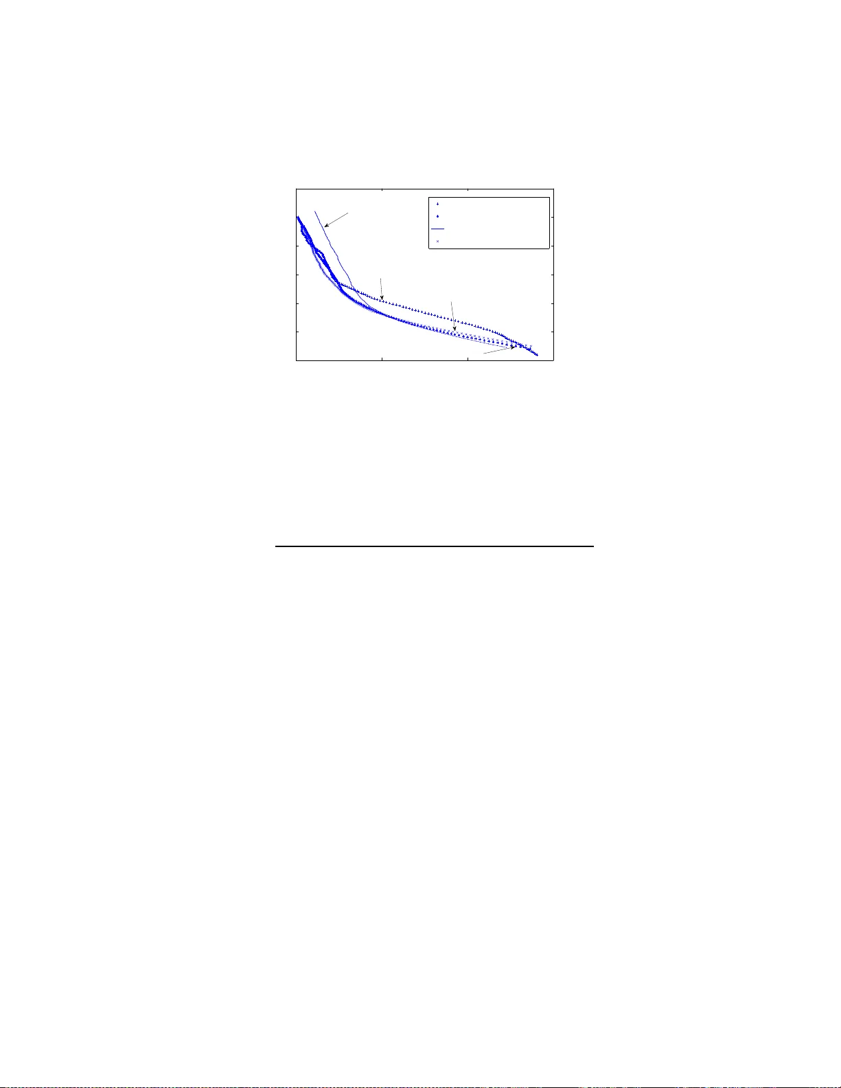
Non-Ba y esian particle filters Alexandre J. Chorin and Xuemin T u Departmen t of Mathematics, Univ ersit y of California at Berk e ley and La wrence Berk eley National Lab oratory Berk eley , CA, 94720 Abstract P article filters for data a ssimilation in nonlinear problems use “par- ticles” (replicas of the underlyin g system) to generate a sequence of probabilit y densit y functions (p dfs) through a Ba y esian pr o cess. This can b e exp ensive b ecause a significant n um b er of particles has to b e used to main tain accuracy . W e offer her e an alternativ e, in whic h the relev ant p dfs are s ampled dir ectly b y an iteration. An example is discussed in detail. Keyw ords pa r t icle filter, c hainless sampling, normalization factor, iter- ation, non-Bay esian 1 In t r o du c tion. There a re many problems in science in whic h the state of a system mus t b e iden tified fro m an uncertain equation supplemen ted b y a stream of no isy data (see e.g. [1]). A natural mo del of this situation consists of a sto c hastic differen tia l equation (SD E): d x = f ( x , t ) dt + g ( x , t ) d w , (1) where x = ( x 1 , x 2 , . . . , x m ) is an m -dimensional ve ctor, d w is m -dimensional Bro wnian motion, f is an m -dimensional v ector function, and g is a scalar (i.e., an m b y m diagonal matrix of the form g I , where g is a scalar and I is the iden tit y mat r ix). The Brow nian motion encapsulates a ll the uncertain ty in this equation. The initial state x (0) is assumed giv en and ma y b e random as we ll. As the experimen t unfolds, it is observ ed, and the v alues b n of a mea- suremen t pro cess are recorded at times t n ; for simplicit y assume t n = nδ , 1 where δ is a fixed time in t erv a l a nd n is an integer. The measuremen ts are related to the evolving state x ( t ) b y b n = h ( x n ) + G W n , (2) where h is a k - dimensional, generally nonlinear, v ector function with k ≤ m , G is a diagonal matrix, x n = x ( nδ ), and W n is a v ector whose comp onents are indep enden t Gaussian v ariables of mean 0 and v ariance 1, indep enden t also of the Brow nian motion in equation (1). The task is to estimate x on the basis of equation ( 1) and the observ ations (2) . If the system (1) is linear a nd the data are Gaussian, the solution can b e found via the Kalman-Bucy filter. In the general case, it is natura l to t r y to estimate x as the mean of its ev olving probability densit y . The initial state x is kno wn and so is its probabilit y densit y; all one has to do is ev aluate sequen tially the densit y P n +1 of x n +1 giv en the probability densit y P n of x n and the data b n +1 . This can b e done b y follo wing “particles” (replicas of the system) whose empirical distribution appro ximates P n . In a Ba y esian filter (see e.g [2, 3 , 4, 5, 6, 7, 8, 9], one uses the p df P n and equation (1) to generate a prior densit y , and then one uses the new data b n +1 to generate a p osterior densit y P n +1 . In addition, one ma y ha v e to sample bac kw ard to tak e in to accoun t the information e ach measuremen t pro vides a b out the past and a v o id ha ving to o man y iden t ical particles. Ev olving pa rticles is typically exp ensiv e, and the backw ard sampling, usually done b y Mark ov chain Monte Carlo (MCMC), can be exp ensiv e as well, b ecause the n um b er of particles needed can grow catastrophically (see e.g. [10]). In this pap er w e offer a n alternativ e to the standard approac h, in whic h P n +1 is sampled directly without recourse t o Ba y es’ theorem and bac kw ard sampling, if needed, is done b y chainles s Mon te Carlo [11 ]. Our direct sam- pling is based on a r epresen tation of a v a r iable with densit y P n +1 b y a col- lection of functions of Gaussian v ariables parametrized by the supp ort of P n , with parameters fo und b y iteratio n. The construction is related to c hainless sampling as described in [11]. The idea in chainle ss sampling is to pr o duce a sample o f a la r g e set of v ariables by sequen tially sampling a grow ing se- quence of nested conditio na lly indep enden t subsets. As observ ed in [12, 13], c ha inless sampling for a SDE reduces to in terp olato r y sampling, as explained b elo w. Our construction will b e explained in the following sections through an example where the p osition o f a ship is deduced from the measuremen ts of an azim uth, already used a s a test b ed in [6, 14, 15]. 2 2 Sampling by in terp olati o n and ite r ati o n. First w e ex plain ho w to sample via in terp olation and iteration in a simple example, related to the example a nd the construction in [12]. Consider the scalar SD E dx = f ( x, t ) dt + √ σ dw ; (3) w e w an t to find sample paths x = x ( t ) , 0 ≤ t ≤ 1, sub ject to the conditions x (0) = 0 , x (1) = X . Let N ( a, v ) denote a Gaussian v ariable with mean a and v ariance v . W e first discretize equation (3) on a regular mesh t 0 , t 1 , . . . , t N , where t n = nδ , δ = 1 / N , 0 ≤ n ≤ N , with x n = x ( t n ), a nd, follow ing [1 2], use a ba lanced implicit discretization [16, 17]: x n +1 = x n + f ( x n , t n ) δ + ( x n +1 − x n ) f ′ ( x n ) δ + W n +1 , where f ′ ( x n , t n ) = ∂ f ∂ x n ( x n , t n ) and W n +1 is N (0 , σ / N ). The joint probability densit y of the v aria bles x 1 , . . . , x N − 1 is Z − 1 exp( − P N 0 V i ), where Z is the normalization constan t and V i = ((1 − δ f ′ )( x n +1 − x n ) − δ f ) 2 2 σ δ = ( x n +1 − x n − δ f / (1 − δ f ′ )) 2 2 σ n , where f , f ′ are functions of the x j , a nd σ n = σ δ / ( 1 − δ f ′ ) 2 (see [18]). O ne can obtain sample solutions b y sampling this densit y , e.g. by MCMC, or one can obta in them by in terp olatio n (chainle ss sampling), as follows . Consider first the sp ecial case f ( x, t ) = f ( t ), so that in particular f ′ = 0. Eac h incremen t x n +1 − x n is no w a N ( a n , σ / N ) v ariable, with the a n = f ( t n ) δ kno wn explicitly . Let N be a pow er of 2. Consider the v ariable x N/ 2 . On one hand, x N/ 2 = N/ 2 X 1 ( x n − x n − 1 ) = N ( A 1 , V 1 ) , where A 1 = P N/ 2 1 a n , V 1 = σ / 2. On the other hand, X = x N/ 2 + N X N/ 2+1 ( x n − x n − 1 ) , 3 so that x N/ 2 = N ( A 2 , V 2 ) , with A 2 = X − N − 1 X N/ 2+1 a n , V 2 = V 1 . The p df of x N/ 2 is the pro duct of the tw o p dfs; o ne can c hec k that exp  − ( x − A 1 ) 2 2 V 1  exp  − ( x − A 2 ) 2 2 V 2  = exp  − ( x − ¯ a ) 2 2 ¯ v  exp( − φ ) , where ¯ v = V 1 V 2 V 1 + V 2 , ¯ a = V 1 A 1 + V 2 A 2 V 1 + V 2 , and φ = ( A 2 − A 1 ) 2 2( V 1 + V 2 ) ; e − φ is the probabilit y of getting from the origin t o X , up to a normalization constan t. Pic k a sample ξ 1 from t he N (0 , 1) densit y; one obt a ins a sample of x N/ 2 b y setting x N/ 2 = ¯ a + √ ¯ v ξ 1 . Giv en a sample of x N/ 2 one can similarly sample x N/ 4 , x 3 N/ 4 , t hen x N/ 8 , x 3 N/ 8 , etc., un til all the x j ha v e b een sampled. If w e define ξ = ( ξ 1 , ξ 2 , . . . , ξ N − 1 ), then for each c hoice of ξ we find a sample ( x 1 , . . . , x N − 1 ) suc h that exp  − ξ 2 1 + · · · + ξ 2 N − 1 2  exp  − ( X − P n a n ) 2 2 σ  = exp  − ( x 1 − x 0 − a 0 ) 2 2 σ / N − ( x 2 − x 1 − a 1 ) 2 2 σ / N − · · · − ( x N − x N − 1 − a N − 1 ) 2 2 σ / N  , (4) where the factor exp  − ( X − P n a n ) 2 2 σ  on the left is the probability o f the fixed end v alue X up to a normalization constan t. In this linear problem, this factor is the same for all the samples a nd therefore harmless. One can r ep eat this sampling pro cess for m ultiple c hoices of the v ariables ξ j ; eac h sample of the corresp onding se t of x n is indep enden t of a n y previous samples o f this set. No w return to the g eneral case. The functions f , f ′ are now functions of the x j . W e obta in a sample of the probability densit y w e w ant b y iteration. First pic k Ξ = ( ξ 1 , ξ 2 , . . . , ξ N − 1 ), where each ξ j is drawn indep enden tly from 4 the N (0 , 1) densit y (this v ector remains fixe d during the iteration). Make a first guess x 0 = ( x 1 0 , x 2 0 , . . . , x N − 1 0 ) (for example, if X 6 = 0, pick x = 0). Ev aluate the functions f , f ′ at x j (note that now f ′ 6 = 0, and therefore the v ariances o f the v arious incremen ts a re no longer constan ts). W e are bac k in previous case, and can find v alues of the incremen ts x n +1 j + 1 − x n j + 1 corresp onding to the v alues of f , f ′ w e ha v e. Rep eat the pro cess starting with the new iterate. If the v ectors x j con v erg e to a v ector x = ( x 1 , . . . , x N − 1 ), w e obtain, in the limit, equation ( 4), where now on the right side σ depends on n so that σ = σ n , and b o th a n , σ n are functions of the final x . The left hand side of (4) b ecomes: exp  − ξ 2 1 + · · · + ξ 2 N − 1 2  exp  − ( X − P n a n ) 2 2 P n σ n  . Note that now the factor exp  − ( X − P n a n ) 2 2 P n σ n  is differen t from sample to sam- ple, and changes the relativ e w eigh ts of the different samples. In av eraging, one should take this factor as w eigh t, o r resample as describ ed at the end of the follow ing section. In order to obta in more uniform weigh ts, one also can use the strategies in [1 1, 12]. One can readily see that the iteration con v erges if K T M < 1, where K is the Lipshitz cons tant of f , T is the length of the in terv al on whic h one w o rks (here T = 1), and M is the maxim um nor m of the vec tors x j + 1 − x j . If this inequalit y is not satisfied for the iteration ab ov e, it can b e re- established b y a suitable underrelaxation. One should course ch o ose N lar g e enough so that the r esults ar e con v erged in N . W e do not pro vide more details here b ecause they are extraneous to our purp ose, whic h is to explain c ha inless/in terp olato ry sampling a nd the use of reference v ariables in a simple con text. 3 The sh i p azim u th pro b lem. The pr o blem w e fo cus on is discuss ed in [6, 14, 15], where it is used to demonstrate the capabilities of particular Ba yes ian filters. A ship se ts out from a p oin t ( x 0 , y 0 ) in the pla ne and undergo es a random w alk, x n +1 = x n + dx n +1 , y n +1 = y n + dy n +1 , (5) 5 for n ≥ 0, and with x 0 = y 0 giv en, and dx n +1 = N ( dx n , σ ), dy n +1 = N ( d y n , σ ), i.e., each displacemen t is a sample o f a Gaussian random v aria ble whose v ariance σ do es not c hange from step to step and whose mean is the v alue of the pr evious displacemen t. An observ er mak es noisy measuremen ts of the azim uth arctan( y n /x n ), recording b n = arctan y n x n + N ( 0 , s ) . (6) where the v ariance s is also fixed; here the observ ed quan tit y b is scalar and is not b e denoted b y a b oldf a ced letter. The problem is to reconstruct t he p ositions x n = ( x n , y n ) from equ ations (5,6). W e tak e the same parameters as [6]: x 0 = 0 . 01 , y 0 = 20, dx 1 = 0 . 002, dy 1 = − 0 . 06, σ = 1 · 10 − 6 , s = 25 · 10 − 6 . W e fo llo w nume rically M particles, all starting from X 0 i = x 0 , Y 0 i = y 0 , as desc rib ed in t he fo llowing sections, and w e estimate the ship’s p osition at time nδ a s the mean o f the lo cations X n i = ( X n i , Y n i ) , i = 1 , . . . , M of the particles at t ha t time. The a uthors of [6] also sho w numeric al results for runs with v arying data and constants; we discuss tho se refinemen ts in section 6 b elo w. 4 F orw ard step. Assume w e ha v e a collection o f M particles X n at time t n = nδ whose empirical densit y approx imates P n ; now w e find incremen ts d X n +1 suc h that the empirical density of X n +1 = X n + d X n +1 appro ximates P n +1 . P n +1 is kno wn implicitly: it is the pro duct of the densit y that can b e deduced f rom the SD E and the o ne that comes f rom t he observ ations, with the a ppropriate normalization. If the incremen ts were kno wn, their probabilit y p (the densit y P n +1 ev aluated at the resulting p o sitions X n +1 ) would b e kno wn, so p is a function of d X n +1 , p = p ( d X n +1 ). F or eac h particle i , w e are go ing to sample a Ga ussian reference densit y , obtain a sample of proba bility ρ , then solv e (b y iteration) the equation ρ = p ( d X n +1 i ) (7) to obtain d X n +1 i . Define f ( x, y ) = arctan( y /x ) and f n = f ( X n , Y n ). W e are working on one par t icle at a time, so the index i can b e temp orarily suppressed. Pick t w o indep enden t samples ξ x , ξ y from a N (0 , 1) density (the reference densit y 6 in the presen t calculation), and set ρ = 1 2 π exp  − ξ 2 x 2 − ξ 2 y 2  ; the v ariables ξ x , ξ y remain unc hanged un til the end of the iteration. W e a re lo oking f o r displacemen ts d X n +1 , d Y n +1 , and parameters a x , a y , v x , v y , φ , suc h tha t : 2 π ρ = exp  − ( dX n +1 − dX n ) 2 2 σ − ( d Y n +1 − d Y n ) 2 2 σ − ( f n +1 − b n +1 ) 2 2 s  exp( φ ) = exp  − ( dX n +1 − a x ) 2 2 v x − ( d Y n +1 − a y ) 2 2 v y  (8) The first equalit y states what we wish to accomplish: find increme nts dX n +1 , d Y n +1 , functions respectiv ely of ξ x , ξ y , whose proba bilit y with resp ect to P n +1 is ρ . The factor e φ is needed to normalize t his term ( φ is called b elo w a “phase”). The second equality sa ys how the goal is reached: w e are lo o king for parameters a x , a y , v x , v y , (all functions of X n ) such that the incremen ts are samples of Gaussian v aria bles with these parameters, with the assumed probabilit y . One should remem b er that in our example the mean of dX n +1 is d X n , and similarly for d Y n +1 . W e are not represen ting P n +1 as a function of a single Gaussian- there is a different Gaussian for every v alue o f X n . T o satisfy the second equalit y w e set up an iteration for vec tors d X n +1 ,j (= d X j for brevit y) that con verges to d X n +1 . Start with d X 0 = 0. W e no w explain ho w to compute d X j + 1 giv en d X j . Appro ximate the o bserv ation equation (6) by f ( X j ) + f x · ( dX j + 1 − dX j ) + f y · ( d Y j + 1 − d Y j ) = b n +1 + N ( 0 , s ) , (9) where the deriv ativ es f x , f y are, like f , ev aluated at X j = X n + d X j , i.e., ap- pro ximate the observ ation equation b y its T ay lor series expansion around the previous iterate. Define a v ariable η j + 1 = ( f x · dX j + 1 + f y · d Y j + 1 ) / p f 2 x + f 2 y . The approx imate observ ation equation says that η j + 1 is a N ( a 1 , v 1 ) v ariable, with a 1 = − f − f x · d X j − f y · d Y j − b n +1 p f 2 x + f 2 y , v 1 = s f 2 x + f 2 y . (10) 7 On the other ha nd, from the equations of motion one finds that η j + 1 is N ( a 2 , v 2 ), with a 2 = ( f x · dX n + f y · d Y n ) / p f 2 x + f 2 y and v 2 = σ . Hence the p df of η j + 1 is, up to normalization factors, exp  − ( x − a 1 ) 2 2 v 1 − ( x − a 2 ) 2 2 v 2  = exp  − ( x − ¯ a ) 2 2 ¯ v  exp( − φ ) , where ¯ v = v 1 v 2 v 1 + v 2 , ¯ a = a 1 v 1 + a 2 v 2 v 1 + v 2 , φ = ( a 1 − a 2 ) 2 2( v 1 + v 2 ) = φ j + 1 . W e can also define a v ariable η j + 1 + that is a linear com bination of dX j + 1 , d Y j + 1 and is uncorrelated with η j + 1 : η j + 1 + = − f y · d Y j + 1 + f x · dX j + 1 p f 2 x + f 2 y . The observ ations do not aff ect η j + 1 + , so its mean and v ariance are known. Giv en the means and v ariances of η j + 1 , η j + 1 + one can easily in v ert the orthog- onal matrix that connects them to dX j + 1 , d Y j + 1 and find the means and v ariances a x , v x of dX j + 1 and a y , v y of d Y j + 1 after their mo dification b y the observ ation (the subscripts on a, v are lab els, not differen tiations). No w one can pro duce v alues for dX j + 1 , d Y j + 1 : dX j + 1 = a x + √ v x ξ x , d Y j + 1 = a y + √ v y ξ y , where ξ x , ξ y are the samples from N (0 , 1 ) c hosen at the b eginning of the iteration. This completes the it eration. This iteration conv erges to X n +1 suc h that f ( X n +1 ) = b n +1 + N (0 , s ), and the phases φ j con v erg e to a limit φ = φ i , where the part icle index i has b een restored. The time in terv al o v er whic h the solution is up dated in eac h step is short, a nd w e do no t expect any problem with conv ergence, either here or in the next section, and indeed t here is none; in all cases the iteration conv erges in a small n um b er of steps. Note that after the it era t io n the v ariables X n +1 i , Y n +1 i are no long er indep enden t- the observ ation creates a relation b etw een them. Do this for all the particles. The particles are now samples of P n +1 , but they hav e b een o btained by sampling differen t densities (remem b er that the parameters in the Gaussians in equation (8) v ary). One can get rid of this het- erogeneit y b y viewing the factors exp( − φ ) as w eigh ts and resampling, i.e., for eac h of M random num b ers θ k , k = 1 , . . . , M dra wn f r om the uniform distri- bution on [0 , 1 ], c ho ose a new ˆ X n +1 k = X n +1 i suc h that Z − 1 P i − 1 j = 1 exp( − φ j ) < 8 θ k ≤ Z − 1 P i j = 1 exp( − φ j ) (where Z = P M j = 1 exp( − φ j )), and then suppress the hat. W e hav e tra ded the resampling of Ba y esian filters fo r a resampling based o n the normalizing factors of the sev eral G aussian densities; this is a w o rth while trade b ecause in a Ba y esian filter one gets a set of samples man y of whic h may hav e low probability with resp ect to P n +1 , and here we hav e a set o f samples eac h one of whic h has high probability with resp ect to a p df close to P n +1 . Note also tha t the resampling do es not ha v e to b e done at ev ery step- for example, one can add up the phases for a giv en part icle and resample only when the ratio of t he largest cum ulativ e weigh t exp( − P φ i ) to the smallest suc h w eigh t exceeds some limit L (the summation is ov er the w eights accrued to a part icular particle i since the last resampling). If one is worried b y to o man y particles b eing close to eac h other (”depletion” in the Ba y esian terminology), one can divide the set of part icles in to subsets of small size and resample only inside those subsets, creating a g reater div ersit y . As will b e seen in section 6, none of these strategies will b e used here and w e will resample fully at ev ery step. 5 Bac kwa rd samplin g . The algorithm of the previous section is sufficien t to create a filter, but accuracy ma y require an additio nal refinemen t. Ev ery observ ation provide s information not only ab o ut the future but also ab out the past- it ma y , for example, ta g as improbable earlier states that had seemed proba ble b efore the observ ation w as made; one ma y ha v e to go ba c k and correct the past after ev ery observ ation (this ba c kw ard sampling is often misleadingly motiv a t ed solely b y the need to create greater div ersit y a mong the particles in a Ba y esian filter). As will b e seen b elo w, this bac kw ard sampling do es not pro vide a significan t b o ost to accuracy in the presen t problem, but it is describ ed here for the sak e a completeness. Giv en a set of particles a t time ( n + 1 ) δ , af ter a forw ard step and maybe a subsequen t resampling, one can figure out where eac h particle i was in the previous t w o steps, and hav e a partial history fo r eac h pa r t icle i : X n − 1 i , X n i , X n +1 i (if resamples had o ccurred, some parts of that history may b e shared amo ng sev eral curren t particles). Kno wing the first and the last mem b er of this sequence , one can in terp olate for the middle term a s in section 2, th us pro- jecting infor ma t ion bac kw ard. This requires that one recompute d X n . 9 Let d X tot = d X n + d X n +1 ; in the presen t section this quan tity is assumed kno wn and remains fixed. In the azim uth problem discussed here , one has to deal with the slight complication due t o t he fact that the mean of eac h incremen t is the v alue of t he previous one, so that t w o successiv e incremen ts are related in a sligh tly more complicated w ay than usual. The displacemen t dX n is a N ( dX n − 1 , σ ) v ariable, and dX n +1 is a N ( d X n , σ ) v ar iable, so that one go es from X n − 1 to X n +1 b y sampling first a (2 dX n − 1 , 4 σ ) v a riable that tak es us f rom X n − 1 to an in termediate p oin t P , with a correction b y the observ ation ha lf w ay up this first leg, and then one samples a N ( dX tot , σ ) v ariable to reach X n +1 , and similarly f o r Y . Let the v a riable that connects X n − 1 to P b e d X new , so that what replaces d X n is d X new / 2. Accordingly , w e are lo o king for a new displacemen t d X new = ( dX new , d Y new ), and for parameters a new x , a new y , v new x , v new y suc h t hat exp  − ξ 2 x + ξ 2 y 2  = exp  − ( dX new − 2 dX n − 1 ) 2 8 σ − ( d Y new − 2 d Y n − 1 ) 2 8 σ  × exp  − ( f n − b n ) 2 2 s  × exp  − ( dX new − dX tot ) 2 2 σ − ( d Y new − dX tot ) 2 2 σ  exp( φ ) = exp  − ( dX new − ¯ a x ) 2 2 v new x − ( d Y new − ¯ a y ) 2 2 v new y  , where f n = f ( X n − 1 + dX new / 2 , Y n − 1 + d Y new / 2) and ξ x , ξ y are indep enden t N (0 , 1) Gaussian v ariables. As in equation (8) , the first equalit y em b o dies what w e wish to accomplish- find incremen ts, functions o f the reference v ari- ables, that sample the new p df at time nδ defined b y the forw ard motion, the constraint imp osed b y the observ ation, and b y kno wledge of the p osition at time ( n + 1) δ t . The second equalit y states that t his is done by finding particle-dep enden t parameters f or a G aussian densit y . W e again find these parameters as w ell as the incremen ts b y iteration. Muc h of the w ork is separate for the X and Y comp onen ts of the equations of motion, so we write some o f the equations for the X comp o nent o nly . Again set up a n iteration for v a r ia bles dX new ,j = dX j whic h con ve rge to dX new . Start with d X 0 = 0. T o find dX j + 1 giv en dX j , approx imate the observ ation 10 equation (6), a s b efore, b y equation (9); define again v aria bles η j + 1 , η j + 1 + , one in the direction o f t he approximate constraint and one orthogona l to it; in the direction of the constrain t multiply the p dfs as in the previous section; construct new means a 1 x , a 1 y and new v a riances v 1 x , v 1 y for dX , d Y at time n , taking in to a ccount the observ a tion at time n , again as b efore. This also pro duces a phase φ = φ 0 . No w tak e in to accoun t that the lo cation of the b oat at time n + 1 is know n; this creates a new mean ¯ a x , a new v ariance ¯ v x , and a new phase φ x , by ¯ v = v 1 v 2 v 1 + v 2 , ¯ a x = a 1 v 1 + a 2 v 2 v 1 + v 2 , φ x = ( a 1 − a 2 ) 2 v 1 + v 2 , where a 1 = 2 a 1 , v 1 = 4 v 1 x , a 2 = X tot , v 2 = σ . Finally , find a new in terp olated p osition dX j + 1 = a new x / 2 + √ v new x ξ x (the calculation for d Y j + 1 is similar, with a phase φ y ), and w e are done. The total phase for in this iteration is φ = φ 0 + φ x + φ y . As the iterates d X j con v erg e to dX new , the phases conv erge to a limit φ = φ i . The probabilit y of a particle arriving at the giv en p osition at time ( n + 1) δ t having b een determined in the forward step, there is no need to resample b efore comparing samples . Once one has the v a lues of X new , a f orw a rd step giv es corrected v alues of X n +1 ; one can use this interpolation pro cess to correct estimates of X k b y subseque n t observ ations for k = n − 1 , k = n − 2 , . . . , as many as are useful. 6 Numerical re s ults. Before presen ting examples of n umerical results for the azimuth problem, we discuss the accuracy one can exp ect. A single set of observ a t ions for our problem relies on 160 samples of a N (0 , σ ) v ar iable. The maxim um lik eli- ho o d estimate of σ give n these samples is a random v ariable with mean σ and standard deviation . 11 σ . W e estimate the unce rtaint y in the p osition of the b oat by pick ing a set of observ ations, then making m ultiple runs of the b oat where the random comp onents of the motion in the direction of the constrain t are fr o zen while the ones orthogonal to it ar e sampled ov er and o v er from t he suitable Gaussian densit y , then computing the distances to the fixed observ ations, es timating the standard deviation of these difference s, and accepting the tra jectory if the estimated standard deviation is within one standard deviation of the nominal v alue of s . This pro cess generates a family of b oat tra jectories compatible with the giv en observ ations. In T able I w e displa y t he standard deviations of the differences b et wee n the r esulting paths and the original path tha t pro duced the observ ations after the num- b er of steps indicated there (t he means of these differences are statistically 11 indistinguishable fro m zero). This T able provides an estimate of the accu- racy w e can exp ect. It is fa ir to assume that these standard deviations are underestimates of t he uncertain ty - a v ariation of a single standar d deviation in s is a strict constrain t, and w e allow ed no v ariatio n in σ . T able I In trinsic uncertaint y in the azim uth problem step x comp onent y comp onent 40 .0005 .21 80 .004 .58 120 .010 .88 160 .017 .95 If o ne w ants reliable informatio n ab out the p erformance of the filter, it is not sufficien t to run the b oat once, record observ ations, and then use the filter to reconstruct the b oat’s path, b ecause the difference b et w een the true path and the r econstruction is a random v ariable whic h may b e acciden tally at ypically small or at ypically larg e. W e ha v e therefore run a large n um b er of suc h reconstructions and computed the means and standard deviations of the discrepancies b etw een path and reconstruction a s a function of the n um b er of steps and of other parameters. In T ables I I and I I I we display the means and standard deviations of these discrepancie s (not of their mean!) in the the x and y comp onen ts of the pa t hs with 2000 runs, at the steps and num b ers of pa r ticles indicated, with no bac kw ard sampling. (Ref. [6] used 100 particles). On the av erage the error is zero, and the error that can b e exp ected in an y one run is of the order of magnitude of the unav oidable error. The standard deviation of the discrepancy is not significan tly smaller with 2 particles that with 100 - the main source of t he discrepancy is the uncertain ty in the data. Most of time one single particle (no resampling) is enough; how ev er, a single par t icle may tempo r a rily stra y in to lo w-probability areas and creates lar ge arguments and n umerical difficulties in the v ar io us functions used in the program. Tw o particles with resampling k eep eac h other within b o unds, because if one of them stra ys it gets replaced b y a replica of t he other. The v arious more sophisticated resampling strategies at the end of section 4 mak e no discernible difference here, and backw ard sampling do es not help m uc h either, b ecause they t o o are unable to remedy the limitatio n of the data set. 12 T able I Ia Mean a nd standard v aria tion of the discrepancy b etw een syn thetic data and their reconstruction, 20 0 0 runs, no bac k step, 100 part icles n. o f steps x comp onent y comp onen t mean s.d. mean s.d. 40 .0004 .04 .0001 .17 80 -.001 .04 -.01 .54 120 -.0008 .07 -.03 1.02 160 -.002 .18 -.05 1.56 T able I Ib Mean a nd standard v aria tion of the discrepancy b etw een syn thetic data and their reconstruction, 20 0 0 runs, no bac k step, 2 pa rticles n. o f steps x comp onent y comp onen t mean s.d. mean s.d. 40 .002 .17 -.0004 .20 80 .01 .43 -.0006 .58 120 .01 .5 7 .009 1.08 160 .006 .5 4 .01 1.67 In Figure 1 w e plot a sample b oat pat h, its reconstruction, and the re- constructions obtained (i) when the initial data for the reconstruction are strongly p erturb ed ( here, the initial data for x, y w ere p erturb ed initially b y , resp ectiv ely , . 1 and . 4 ) , and (ii) when t he v alue of σ a ssumed in the recon- struction is random: σ = N ( σ 0 , ǫσ 0 ), where σ 0 is the constan t v alue used un til no w and ǫ = 0 . 4 but the calculation is otherwise identical. This produces v ariations in σ of the o rder of 40 %; any larger v ariance in the p erturbations pro duced negativ e v alue of σ . The differences betw een the reconstructions and the true pa t h remain w ithin the acc eptable rang e of erro rs. The se graphs sho w that the filter has little sensitivit y to perturbatio ns (w e did not calculate statistics here b ecause the insensitivit y holds for eac h individual run). W e now estimate the parameter σ from data . The filter needs an esti- mate of σ to function, call this estimate σ assumed . If σ assumed 6 = σ , the other assumptions used to pro duce the data set (e.g. indep endence of the displace- men ts and of the observ ations) a re also false, and all one has to do is detect 13 0 0.5 1 1.5 10 12 14 16 18 20 22 X Y (1) boat path (2) its reconstruction (3) its reconstruction (i) (4) its reconstruction (ii) (4) (1) (3) (2) Figure 1: Some b oat tra jectories (explained in the text) the fallacy . W e do it b y pic king a tra jectory of a particle and computing the quan tit y D = ( P J 2 ( dX j + 1 − dX j )) 2 + ( P J 2 ( d Y j + 1 − d Y j )) 2 P J 2 ( dX j + 1 − dX j ) 2 + P J 2 ( d Y j + 1 − d Y j ) 2 . If the increm en ts are independen t then on the av erage D = 1; w e will try to find the real σ b y finding a v alue of σ assumed for whic h this happ ens. W e c ho se J = 40 (the early part of a t ra jectory is less noisy than the later par t s). As w e already kno w, a single run cannot prov ide an accurate estimate of σ , and accuracy in the reconstruction dep ends o n ho w man y runs are used. In T able I I I w e displa y some v alues of D a v eraged o v er 200 and ov er 5000 runs as a function of the ratio of σ assumed to the v alue o f σ used to generate the data. F rom the longer computation one can find the correct v alue of σ with an erro r of ab out 3%, while with 200 runs the uncertain ty is ab out 10 %. T able I I I The mean of the discriminan t D as a function of σ assumed /σ , 30 particles 14 σ assumed /σ 5000 runs 200 runs .5 1.14 ± .01 1.21 ± .08 .6 1.08 ± .01 1.14 ± .07 .7 1.05 ± .01 1.10 ± .07 .8 1.04 ± .01 1.14 ± .07 .9 1.00 ± .01 1.01 ± .07 1.0 1.00 ± .01 .96 ± .07 1.1 .97 ± .01 1.01 ± .07 1.2 .94 ± .01 .99 ± .0 7 1.3 .93 ± .01 1.02 ± .07 1.4 .90 ± .01 .85 ± .0 6 1.5 .89 ± .01 .93 ± .0 7 2.0 .86 ± .01 .78 ± .0 5 7 Conclus ions. W e ha ve exhibite d a non-Bay esian filtering metho d, related to recen t w ork on c ha inless sampling, designed to fo cus pa rticle paths more sharply and thus require few er of them, at the cost of an added complexity in the ev aluation of eac h path. The main features of the algor it hm are a represen ta t io n of a new p df by means of a set of functions of Gaussian v ariables and a resampling based on normalizat io n fa ctors. The construction w as demonstrated on a standard ill-conditioned test problem. F urther applications will b e published elsewhere . 8 Ac kn owledgmen t s. W e would lik e to thank Prof. R. Kupferman, Prof. R. Miller, and Dr. J. W eare fo r a sking searching questions and providing go o d advice. This work w a s supported in part b y the Director, O ffice of Science, Computational and T ec hnology Researc h, U.S. D epartmen t of Energy under Contract No. DE-A C02-05CH112 31, and b y the Natio nal Science F oundatio n under gr an t DMS-070591 0. 15 References [1] Doucet, A., de F reitas, N., and Gordon, N. (eds) (2001), Sequen tial Mon te Carlo Metho ds in Practice, Spring er, New Y ork. [2] Maceac hern, S., Clyde, M., and Liu, J. (1999), C an. J. Stat. 27:251–2 6 7. [3] Liu, J. and Sabati, C. (200 0), Biome trika 87:353–369. [4] Doucet, A., Go dsill, S., a nd Andrieu, C. (20 00), Stat. Comp. 10:197–208. [5] Arulampalam, M., Mask ell, S., Gordon, N., and Clapp, T. (2002) , IEEE T r a ns. Sig. Pr o c. 50:174–188 . [6] Gilks, W. and Berzuini, C. (20 01), J. R oy. Statist. So c. B 63:127 –146. [7] Chorin, A.J. and Krause, P . (20 04), Pr o c. Nat. A c ad. Sci. USA 101:15013 –15017. [8] Do wd, M. (200 6), Envir on metrics 17:435–45 5 . [9] Doucet, A. a nd Johansen, A., P article Filtering and Smoo thing: Fif- teen years Later, Handb o ok o f Nonlinear Filtering (eds. D. Crisan et B. Rozo vsky), Oxford Unive rsit y Press, to app ear. [10] Sn yder, C., Bengtsson, T., Bic k el, P , and Anderson, J. (2008), Mon. We a. R ev. 1 36:4629–46 40. [11] Chorin, A.J. (2008), Comm . Appl. Math. Comp. Sc. 3:77– 93. [12] W eare, J. (200 7), Pr o c. Nat. A c ad. Sc. USA 1 04:12657–1 2662. [13] W eare, J., P article filtering with path sampling and a n a pplication to a bimo dal o cean curren t mo del, in press, J. Comput. Ph ys. [14] Gordon, N., Salmond, D., and Smith A. (1993), I EEE Pr o c e e dings-F 140: 1 07–113. [15] Carp en ter, J., Clifford, P ., and F earnhead, P . (1999 ) IEEE Pr o c e e dings- R adar Sonar and Navigation 146:2 –7. [16] Milstein, G., Platen, E., and Sc h urz H. (1998), SI AM J. Num. Anal. 35:1010–1 019. 16 [17] Klo eden, P . and Platen, E. (1992), Numerical Solution of Sto c hastic Differen tial Equations, Springer, Berlin. [18] Stuart, A., V oss, J., and Wilb erg, P . ( 2 004), Com m. Math. Sc. 4:685– 697. 17