Polynomial Linear Programming with Gaussian Belief Propagation

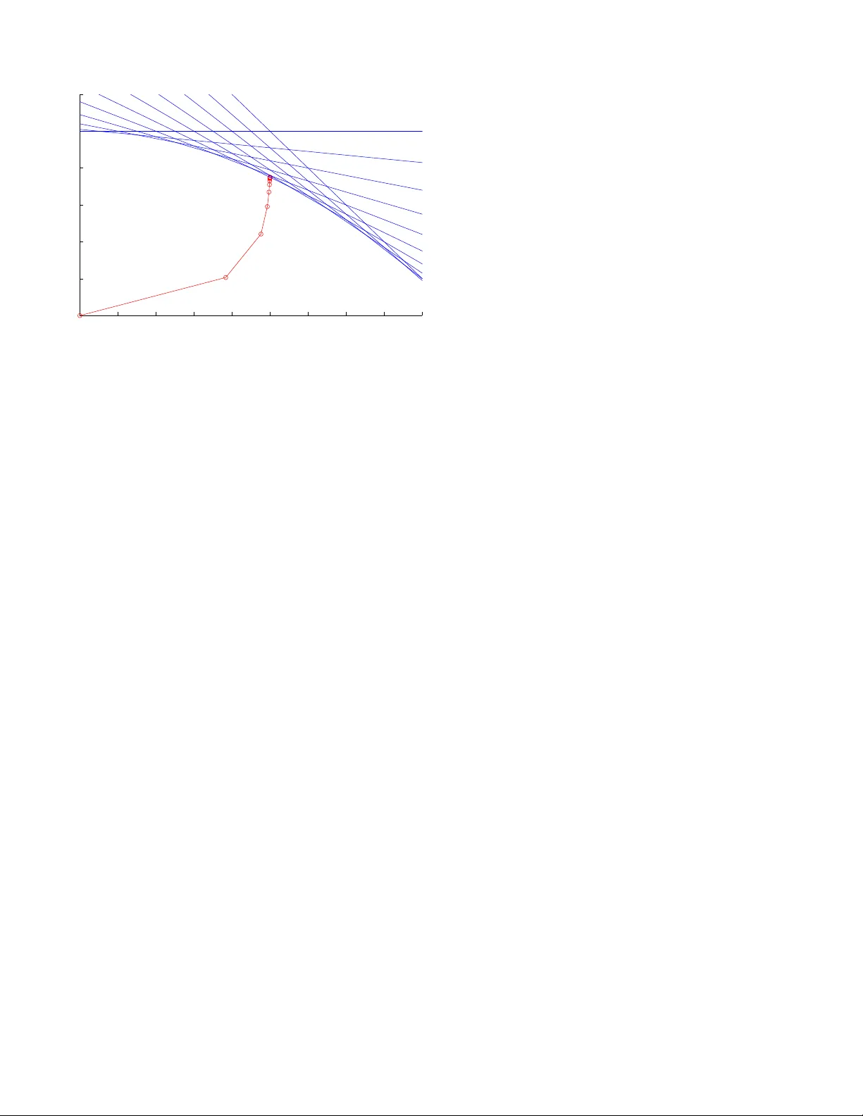
Polynomial Linear Programming with Gaussian Belief Propagation Danny Bickson, Y oav T ock IBM Haifa Resear ch Lab Mount Carmel Haifa 31905, Israel Email: { dannybi,tock } @il .ibm.com Ori S hental Center for Magnetic Recording Researc h UCSD, San Diego 9500 Gilman Driv e La Jolla, CA 92093, USA Email: oshental@ucsd. edu Danny Dole v School of Computer Science and Engineering Hebre w Univ ersity of Jerusalem Jerusalem 91904, Israel Email: dolev@cs.huji.ac.il Abstract —Interior -point methods are state- of-the-a rt al- gorithms f or solving linear programming (LP) problems with polyno mial complexit y . Specifically , the K armarkar algorithm typically solves LP problems in time O ( n 3 . 5 ) , where n is the number of unknown v ariables. Karmarkar’s celebrated a lgorithm is known to be an instance of the log-barrier method using the Newton iteratio n. The main computationa l overhead of this met hod is in in verting the Hessian matrix of the Newton iteration. In t his contribution, we propose the applicatio n of the Ga ussian belief propagation (GaBP) alg orithm a s part of an efficient and dis tributed LP solver that exploits t he sparse and symmetric structure of the Hessian matrix and av oids the need for direct matr ix inversion. This approach shifts the computation f rom realm of linear algebra to that of proba- bilistic inference on graphical models, thus applying GaBP as an efficient inference engine. Our construction is general and can be used for a ny interior-point algorithm which uses t he Newto n method, including non-linear program solvers. I . I N T R O D U C T I O N In recent years, cons iderable attent ion has been dedicated to the relation b etween belief propagation message pass ing and linear programming s chemes. This relation is natural since the maximum a- posteriori (MAP) in ference problem can be t rans- lated into i nteger linear programmin g (ILP) [1]. W eiss et al. [1] approximate the solu tion to the ILP probl em by relaxing it to a LP problem usin g con vex variational methods. In [2], tree-re weighted belief propagation (BP) is used to find the global minimum of a con ve x approximation to the free ener gy . Both of these works apply discrete forms of BP . Globerson et al. [3], [4] assum e con ve xity of the prob lem and modi fy the BP update rul es using dual-coordi nate ascent algori thm. Hazan et al. [5] describe an algo rithm for s olving a general con vex free energy min imization. In both cases the algorithm i s guaranteed to con ver ge to the global minimum as t he problem is tailored to b e conv ex. In the present work we take a differe nt path. Un - like m ost of the pre vious work which uses gradient- descent methods, we s how how t o use int erior -point methods which are shown to hav e strong advantages over gradient and steepest descent m ethods. (For a comparativ e study see [6, § 9 . 5 ,p. 49 6].) Th e main benefit of using interior point m ethods is their rapid con vergence, which is quadratic once we are close enough to the optim al solution. Their main drawback is that t hey require heavier com putational ef fort for formin g and in verting the Hessian ma- trix, n eeded for computing t he Newton step. T o overc ome this, we propose the use of Gaussian BP (GaBP) [7], [8], which i s a variant o f BP applicable when the underlyi ng distribution is Gaussian. Usin g GaBP , we are able to reduce the time associated with the Hessian inv ersion task, from O ( n 2 . 5 ) to O ( np log( ǫ ) / lo g( γ )) at the worst case, where p < n is the size o f the constraint matrix A , ǫ is th e desired accuracy , and 1 / 2 < γ < 1 i s a parameter characterizing the matrix A . This computati onal saving is accomplished by exploiting the sparsi ty of the Hess ian matrix. An add itional b enefit of our GaBP-based ap- proach i s that the polynomial-com plexity LP solver can be imp lemented i n a di stributed manner , en- abling ef ficient solution of large-sca le problems. W e also provide what we belie ve is the first theoretical analysi s of the con vergence speed of the GaBP algorithm. The paper is organized as foll ows. In Section II, we reduce standard lin ear programm ing to a least-squares probl em. Section III shows how t o solve t he least-squ ares problem using t he GaBP algorithm. In Section IV, we extend our construction to the primal-dual metho d. W e give our con ver gence results for the GaBP algorit hm in Section V, and demonstrate our construction in Section VI us ing an elementary example. W e p resent our conclusions in Section VII. I I . S T A N DA R D L I N E A R P RO G R A M M I N G Consider th e standard li near p rogram minimize x c T x (1a) subject to Ax = b , x ≥ 0 (1b) where A ∈ R n × p with rank { A } = p < n . W e assume the problem is solvable with an optimal x ∗ assignment. W e also assume that the problem is strictly fea sible, or in other words there exists x ∈ R n that s atisfies Ax = b and x > 0 . Using the log-barrier m ethod [6, § 11 . 2 ], one gets minimize x ,µ c T x − µ Σ n k =1 log x k (2a) subject to Ax = b . (2b) This is an approxi mation to the origi nal problem (1a). The quality o f the approximati on improves as the parameter µ → 0 . Now we would like t o use the Newton method in for solvi ng the log -barrier constrained ob jectiv e function (2a ), described in T able I. Suppose t hat we hav e an initi al feasible point x 0 for the canoni cal linear program (1a). W e approximate the obj ectiv e function (2a) around the curre nt point ˜ x using a second-order T aylor expansion f ( ˜ x + ∆ x ) ≃ f ( ˜ x ) + f ′ ( ˜ x )∆ x + 1 / 2∆ x T f ′′ ( ˜ x )∆ x . (3) Finding the optimal search direction ∆ x yields the computation of the gradient and compare it to zero ∂ f ∂ ∆ x = f ′ ( ˜ x ) + f ′′ ( ˜ x )∆ x = 0 , (4) ∆ x = − f ′′ ( ˜ x ) − 1 f ′ ( ˜ x ) . (5) Denoting the current po int ˜ x , ( x , µ, y ) and the Ne wton step ∆ x , ( x , y , µ ) , we compute the gradient f ′ ( x , µ, y ) ≡ ( ∂ f ( x , µ, y ) /∂ x , ∂ f ( x , µ, y ) /∂ µ, , ∂ f ( x , µ, y ) /∂ y ) The Lagrangian is L ( x , µ, y ) = c T x − µ Σ k log x k + y T ( b − Ax ) , (7) ∂ L ( x , µ, y ) ∂ x = c − µ X − 1 1 − y T A = 0 , (8) ∂ 2 L ( x , µ, y ) ∂ x = µ X − 2 , (9) where X , diag ( x ) and 1 is the all-one colum n vector . Substit uting (8)-(9) into (4), we get c − µ X − 1 1 − y T A + µ X − 2 x = 0 , (10) c − µ X − 1 1 + x µ X − 2 = y T A , (11) ∂ L ( x , µ, y ) ∂ y = Ax = 0 . (12) Now multipl ying (11) by AX 2 , and using (12) to eliminate x we get AX 2 A T y = AX 2 c − µ AX 1 . (13) These normal equ ations can be recognized as gen- erated from the l inear least-squares p roblem min y || XA T y − Xc − µ A X1 || 2 2 . (14) Solving for y we can compute the Ne wton direction x , taking a step towar ds the boundary and compose one iteration of the Ne w ton algorithm. Next, we will explain how to shift the deterministic LP problem to the probabili stic do main and solve i t dist ributi vely using GaBP . T ABLE I T H E N E W T O N A L G O R I T H M [ 6 , § 9 . 5 . 2 ] . Giv en feasible starting point x 0 and tolerance ǫ > 0 , k = 1 Repeat 1 Compute the Newton step and decrement ∆ x = f ′′ ( x ) − 1 f ′ ( x ) , λ 2 = f ′ ( x ) T ∆ x 2 Stopping criterion. quit if λ 2 / 2 ≤ ǫ 3 Line search. Choose step size t by backtracking line search. 4 Update. x k := x k − 1 + t ∆ x , k = k + 1 I I I . F RO M L P T O P R O BA B I L I S T I C I N F E R E N C E W e start from the least-squares prob lem (14), changing notations t o min y || Fy − g | | 2 2 , (15) where F , X A T , g , X c + µ A X1 . Now we define a multiv ariate Gauss ian p ( ˆ x ) , p ( x , y ) ∝ exp( − 1 / 2( Fy − g ) T I ( Fy − g )) . (16) It is clear that ˆ y , the m inimizing s olution of (15), is the MAP est imator of the cond itional probability ˆ y = arg max y p ( y | x ) = = N (( F T F ) − 1 F T g , ( F T F ) − 1 ) . (17) Recent results by Bickson and Shental et al. [7]– [9] show t hat t he pseudoin verse problem (17) can be computed efficiently and di stributi vely by usin g the GaBP alg orithm. The formulation (16) allows us to shi ft the l east- squares problem from an algebraic t o a probabil istic domain. Inst ead of sol ving a determi nistic vector - matrix linear equati on, we now solve an inference problem i n a graphical model describing a certain Gaussian d istribution functi on. Following [9] we define t he joint cov ariance matrix C ,  − I F F T 0  (18) and the s hift vector b , { 0 T , g T } T ∈ R ( p + n ) × 1 . Giv en the covariance matri x C and the shift vector b , one can write explicitly the Gaussian density functi on, p ( ˆ x ) , and its corresponding graph G with edge potentials (‘compatibilit y functions’) ψ ij and self-potentials (‘evidence’) φ i . These graph potentials are determined according to th e follow- ing pai rwise factorization o f the Gaussian distribu- tion p ( x ) ∝ Q n i =1 φ i ( x i ) Q { i,j } ψ ij ( x i , x j ) , resulting in ψ ij ( x i , x j ) , exp( − x i C ij x j ) , and φ i ( x i ) , exp  b i x i − C ii x 2 i / 2  . The set of edges { i, j } cor- responds to the set of non-zero entries in C (18 ). Hence, we would like to calculate the marginal densities, wh ich must als o be Gaussian, p ( x i ) ∼ N ( µ i = { C − 1 g } i , P − 1 i = { C − 1 } ii ) , ∀ i > p, where µ i and P i are the marginal m ean and inv erse var iance (a.k.a. p recision), respectiv ely . Recall that, according t o [9], the inferred m ean µ i is identical to t he desired solution ˆ y of (17). The GaBP update rules are summarized in T able II. It is known that if GaBP con verges, it results in exact inference [10]. Howe ver , in contrast to con- ventional iterative metho ds for the so lution of sys - tems of l inear equations, for GaBP , determi ning the exact region of con ve r gence and con ve r gence rate remain open research problems. All that is known is a sufficient (but not necessary) condi tion [11], [12] stating that GaBP conv er ges when the spectral ra- dius satisfies ρ ( | I K − A | ) < 1 . A stricter sufficient condition [10], determines that the matrix A mus t be diagonally do minant ( i.e. , | a ii | > P j 6 = i | a ij | , ∀ i ) in o rder for GaBP to con ve r ge. Con vergence speed is d iscussed in Section V. I V . E X T E N D I N G T H E C O N S T RU C T I O N T O T H E P R I M A L - D UA L M E T H O D In the pre vious section we hav e shown how to compute one it eration of the Newton m ethod using GaBP . In thi s section we extend the technique for T ABLE II C O M P U T I N G x = A − 1 b V I A G A B P [ 7 ] . # Stage Operation 1. Initial ize Compute P ii = A ii and µ ii = b i / A ii . Set P k i = 0 and µ k i = 0 , ∀ k 6 = i . 2. Iterate P ropagate P k i and µ k i , ∀ k 6 = i such th at A k i 6 = 0 . Compute P i \ j = P ii + P k ∈ N ( i ) \ j P k i and µ i \ j = P − 1 i \ j ( P ii µ ii + P k ∈ N( i ) \ j P k i µ k i ) . Compute P ij = − A ij P − 1 i \ j A j i and µ ij = − P − 1 ij A ij µ i \ j . 3. Chec k If P ij and µ ij did not conv er ge, return t o #2. Else, con tinue to #4 . 4. Infer P i = P ii + P k ∈ N( i ) P k i , µ i = P − 1 i ( P ii µ ii + P k ∈ N( i ) P k i µ k i ) . 5. Output x i = µ i computing the primal-dual m ethod. This construc- tion i s attractiv e, since the extended techniqu e has the same computation overhe ad. The dual p roblem ( [13]) conforming to (1a) can be computed using t he Lagrangian L ( x , y , z ) = c T x + y T ( b − Ax ) − z T x , z ≥ 0 , g ( y , z ) = inf x L ( x , y , z ) , (19a) subject to Ax = b , x ≥ 0 . (19b) while ∂ L ( x , y , z ) ∂ x = c − A T y − z = 0 . (20) Substitutin g (20 ) into (19a) we get maximize y b T y subject to A T y + z = c , z ≥ 0 . Primal op timality is o btained u sing (8) [13] y T A = c − µ X − 1 1 . (22) Substitutin g (22) in (21a) we g et the connection between the p rimal and dual µ X − 1 1 = z . In total, we ha ve a prim al-dual system (again we assume that the soluti on is strictly feasible, namely x > 0 , z > 0 ) Ax = b , x > 0 , A T y + z = c , z > 0 , Xz = µ 1 . The solution [ x ( µ ) , y ( µ ) , z ( µ )] of these equ ations constitutes t he central path of solu tions to t he log- arithmic barrier method [6, 11.2.2]. App lying the Ne wton method to this system of equ ations we get   0 A T I A 0 0 Z 0 X     ∆ x ∆ y ∆ z   =   b − A x c − A T y − z µ 1 − Xz   . (24) The solution can be computed explicitl y by ∆ y = ( AZ − 1 XA T ) − 1 · ( AZ − 1 X ( c − µ X − 1 1 − A T y ) + b − Ax ) , ∆ x = X Z − 1 ( A T ∆ y + µ X − 1 1 = c + A T y ) , ∆ z = − A T ∆ y + c − A T y − z . The main compu tational overhead in this m ethod is t he comp utation of ( AZ − 1 XA T ) − 1 , whi ch is deriv ed from the Newton step in (5). Now we would like to use GaBP for computing the solution. W e make the fol lowing si mple change to (24) to make it symmetric: s ince z > 0 , we can multiply the third row by Z − 1 and get a modified symmetric sy stem   0 A T I A 0 0 I 0 Z − 1 X     ∆ x ∆ y ∆ z   =   b − Ax c − A T y − z µ Z − 1 1 − X   . Defining ˜ A ,   0 A T I A 0 0 I 0 Z − 1 X   , and ˜ b ,   b − Ax c − A T y − z µ Z − 1 1 − X   . one can use GaBP iterativ e algorithm s hown in T able II. In general, by looking at (4) we see that the solution o f each Newton step in volv es in verting th e Hessian matrix f ′′ ( x ) . The state-of-the-art approach in practical imp lementations of the Ne wton s tep is first comp uting t he Hessian in verse f ′′ ( x ) − 1 by using a (sparse) decomposi tion m ethod l ike (sparse) Cholesky decomposit ion, and then multipl ying the result by f ′ ( x ) . In our approach, t he GaBP al- gorithm computes directly the result ∆ x , without computing the ful l matrix in verse. Furthermore, if the GaBP algorit hm con ver ges, t he comput ation of ∆ x is guaranteed to be accurate. V . N E W C O N V E R G E N C E R E S U L T S In thi s section we give an upper boun d on the con vergence rate of the GaBP algo rithm. As far as we kn ow this is the first theoretical result b ounding the con ve r gence s peed of the GaBP algorithm. Our upper bound is based on the work of W eiss et al. [10, Claim 4 ], which proves th e correctness of the m ean computati on. W eiss uses th e pairwise potentials form 1 , where p ( x ) ∝ Π i,j ψ ij ( x i , x j )Π i ψ i ( x i ) , ψ i,j ( x i , x j ) ≡ exp( − 1 / 2( x i x j ) T V ij ( x i x j )) , V ij ≡  ˜ a ij ˜ b ij ˜ b j i ˜ c ij  . Assuming the opti mal solutio n is x ∗ , for a desi red accurac y ǫ || b || ∞ where || b || ∞ ≡ max i | b i | , and b is the shift vector , we need to run the algorithm for at most t = ⌈ log ( ǫ ) / lo g( β ) ⌉ rounds to get an accuracy of | x ∗ − x t | < ǫ || b || ∞ where β = max ij | ˜ b ij / ˜ c ij | . The problem with appl ying W eis s’ result di rectly to our m odel is that we are working with different parameterizations. W e use the informat ion for m p ( x ) ∝ exp( − 1 / 2 x T Ax + b T x ) . The decomposition of the matrix A in to pairwise potentials is not unique. In order to use W eiss’ result, we propose such a decomposit ion. Any decomp osition from the canonical form to t he pairwi se p otentials form should be subject to t he following constraints [10] ˜ b ij = A ij , Σ j ˜ c ij = A ii . W e propose to init ialize the pairwise potentials as following. Assum ing t he matrix A is diagonally 1 W eiss assumes scalar variables wi th zero means. dominant, we define ε i to b e t he non negati ve gap ε i , | A ii | − Σ j | A ij | > 0 . and the fol lowing decomposition ˜ b ij = A ij , ˜ c ij = A ij + ε i / | N ( i ) | , where | N ( i ) | is the num ber o f graph neighbors of node i . Following W eiss, we define γ to be γ = max i,j | ˜ b ij | | ˜ c ij | = | a ij | | a ij | + ε i / | N ( i ) | = = max i,j 1 1 + ( ε i ) / ( | a ij || N ( i ) | ) < 1 . (25) In total, we get that for a desired accuracy of ǫ || b || ∞ we need to iterate for t = ⌈ log( ǫ ) / log ( γ ) ⌉ rounds. Note that this is an up per bound and in practice we indeed have observed a much faster con vergence rate. The computation of the parameter γ can be easil y done in a distributed manner: Each nod e locally computes ε i , and γ i = max j 1 / (1 + | a ij | ε i / N ( i )) . Finally , one maximum operation is p erformed glob- ally , γ = max i γ i . A. Applications to Interior-P oint Methods W e would like to compare the running time of our proposed method to the Newton interior-point method, utilizing our ne w con vergence results of the pre vi ous s ection. As a reference we take t he Karmarkar algorithm [14] which is kn own to be an i nstance of the Newton met hod [15]. Its running time is composed of n rounds, where on each roun d one Ne wton step is computed. Th e cost of com put- ing on e Newton step on a dense Hessian matrix is O ( n 2 . 5 ) , so the to tal runn ing t ime i s O ( n 3 . 5 ) . Using our app roach, the total numb er of Newton iterations, n , remains th e sam e as in the Karmarkar algorithm. Howe ver , we exploit the special structure of the Hessian matrix, which is both symm etric and sparse. Assum ing that the si ze of the con straint matrix A i s n × p, p < n , each iteratio n of GaBP for computing a single N e wton step take s O ( np ) , and based on our new con ver gence analysis for accuracy ǫ || b || ∞ we need to iterate for r = ⌈ log( ǫ ) / log ( γ ) ⌉ rounds , where γ i s defined in (25). The tot al computati onal burde n for a single Newton step is O ( np log( ǫ ) / log( γ )) . T here are at most n rounds, hence in tot al we get O ( n 2 p log( ǫ ) / lo g ( γ )) . 0 0.1 0.2 0.3 0.4 0.5 0.6 0.7 0.8 0.9 0 0.2 0.4 0.6 0.8 1 1.2 x1 x2 Fig. 1. A simple example of using GaBP for solving li near programming with two variables and elev en constraints. Each red circle shows one iteration of the Ne wton method . V I . E X P E R I M E N TA L R E S U LT S W e dem onstrate the applicabili ty of the propo sed algorithm using the following simple linear program borrowed from [16] maximize x 1 + x 2 subject to 2 px 1 + x 2 ≤ p 2 + 1 , p = 0 . 0 , 0 . 1 , · · · , 1 . 0 . Fig. 1 shows execution of the affine-scaling al- gorithm [17], a variant of Karmarkar’ s algorithm [14], on a small problem wit h two variables and ele ven const raints. Each circle i s one Newton step. The in verted Hessian is computed u sing t he GaBP algorithm, us ing two computing nodes. M atlab code for this example can be downloaded from [18]. Regarding larger scale problems, we hav e ob- served rapid con ver g ence (of a single Ne wton step computation) on very large scale problems. For example, [19] demons trates con ver g ence of 5-10 rounds on sp arse constraint m atrices with several millions of variables. [20] shows con ver gence of dense constraint m atrices of size up to 150 , 000 × 150 , 000 in 6 roun ds, where t he algorithm is run in parallel using 1, 024 CPUs. Em pirical comparison with other iterative algorith ms is given in [8]. V I I . C O N C L U S I O N In this paper we hav e shown how to efficiently and dist ributi vely solve interior-point methods using an i terativ e algorit hm, t he Gaus sian belief p ropaga- tion algorithm. Unli ke previous approaches w hich use di screte b elief propagatio n and gradient descent methods, we t ake a different path by using con- tinuous beli ef propagation appli ed t o interior-point methods. By shiftin g the Hessian matrix in verse computation required by the Newton method, from linear algebra domain to the probabilisti c domain, we gain a significant speedup in performance of the Newton method. W e believe there are numerous applications that can benefit f rom our ne w approach. A C K N OW L E D G E M E N T O. Shental acknowledges t he partial s upport of the NSF (Grant CCF-0514859). D. Bickson would like to thank Nati Linial from the Hebrew Univ ersity of Jerusalem for proposing t his research di rection. The authors are grateful to Jack W olf and Paul Siegel from UCSD for useful discussi ons and for constructive comment s on the manuscript. R E F E R E N C E S [1] C. Y ano ver , T . Meltzer, and Y . W eiss, “Li near programming relaxations and belief propagation – an empirical study , ” in J ournal of Machine Learning Resear ch , vol. 7. Cambridge, MA, US A: MIT Press, 200 6, pp. 1887–1907. [2] Y . W eiss, C. Y anover , and T . Meltzer , “Map estimation, linear programming and b elief pro pagation with co n v ex free energies, ” in The 23th Confer ence on Uncertainty in A rtificial Intelligence (U AI) , 2007. [3] A. Globerson and T . Jaakkola, “F ixing max-product: Conv er- gent message passing algorithms for map lp-relaxations, ” in Advances i n Neural Information Proce ssing Systems (NIPS) , no. 21, V ancouver , Canada, 2007. [4] M. Collins, A. Globerson, T . Koo , X. Carreras, and P . Bartlett, “Exponentiated gradient algorithms for conditional rando m fields and max-margin markov networks, ” in Journ al of Ma- chine Learning Resear ch. Accepted for publication , 2008. [5] T . Hazan and A. Shashua, “Con vergent message-passing al- gorithms for inference over general graphs wi th con vex free energy , ” in The 24th Confer ence on Uncertainty in Artificial Intelligence (UAI) , Helsinki, July 2008. [6] S. Boyd and L. V andenberghe, Con vex Optimization . Cam- bridge University Press, March 2004. [7] O. Shental, D. Bickson, P . H. Siegel, J. K. W olf, and D. Dolev , “Gaussian belief propagation solver for systems of linear equa- tions, ” in IE EE Int. Symp. on Inform. Theory (ISIT) , T oronto, Canada, July 2008. [8] D. Bickson, O. Shental, P . H. Siegel, J. K. W olf, and D. Dolev , “Linear detection via belief propagation , ” in Pr oc. 45th Allerton Conf. on Communications, Contr ol and Computing , Monticello, IL, US A, Sept. 2007. [9] ——, “Gaussian belief propagation based multi user detection, ” in IEEE Int. Symp. on Inform. Theory (ISIT) , T oronto, Canada, July 200 8. [10] Y . W eiss and W . T . Freeman, “Correctness of belief propagation in G aussian graphical models of arbitr ary topology , ” Neural Computation , vol. 13, no. 10, pp. 2173–22 00, 2001. [11] J. K. Johnson, D. M. Malioutov , and A. S. Willsky , “W alk- sum interpretation and analysis of Gaussian belief propag ation, ” in Advances in Neural Information Proc essing Systems 18 , Y . W eiss, B . Sch ¨ olkop f, and J. Platt, Eds. Cambridge, MA: MIT P ress, 200 6, pp. 579–586. [12] D. M. Malioutov , J. K. Johnson, and A. S. W illsky , “W alk-sums and belief propagation in Gaussian graphical models, ” Journal of Mac hine L earning Researc h , vol. 7, Oct. 2006. [13] S. Portno y and R. Koen ker , “The gaussian hare and the laplacian tortoise: Computability of squared- error versus absolute-error estimators, ” in Statistical Science , vo l. 12, no. 4. Institute of Mathematical S tatistics, 199 7, pp. 279–296. [14] N. Karmarkar , “ A new polynomial-time algorithm f or li near programming, ” in STOC ’84: P r oceed ings of the si xteenth annual ACM symposium on T heory of computing . New Y ork, NY , USA: A CM, 1984, pp. 302– 311. [15] D. A. Bayer and J. C. Lagarias, “Karmarkar’ s li near pro- gramming algorithm and ne wton’ s method, ” in Mathematical Pr og ramming , vol. 50, no. 1, March 1991, pp. 291–330 . [16] http://en.wikipedia. org/wiki/Karm arkar’s_algorithm . [17] R. J. V ande rbei, M. S. Meketon, and B. A. Freedman, “ A modification of karmarkar’ s linear programming algorithm, ” in Algorithmica , vol. 1, no. 1, March 1986, pp. 395–407. [18] http://www.cs.huji.a c.il/labs/dan ss/p2p/gabp/ . [19] D. Bickson and D. Malkhi, “ A unifying framework for rating users and data items in peer-to-peer and social networks, ” in P eer -to-P eer Networking and Applications (PPNA) Jou rnal, Spring er-V erlag , April 2008. [20] D. Bickson, D. Dolev , and E. Y om-T ov , “ A gaussian belief propagation solver for large scale support vector machines, ” in 5th Eur opean Confer ence on Complex Systems , Jerusalem, Sept. 200 8.