Fountain Codes and Invertible Matrices

F OUNTAIN codes were first mentioned in [1]. LT-codes [3] are first practical Fountain codes. In Fountain codes we have k input symbols and n output symbols. We call an encoding graph a bipartite graph where on the other side are the input symbols and on the other side the output symbols. There are edges which mark the connections between the input symbols and the output symbols. We call the degree of an output symbol the number of input symbols the output symbol is connected to. The degree distribution ρ(i) tells the probability that an output symbol has i connections. We call an encoding matrix R a k × k matrix where an element r lm is 1 if the m:th input symbol affects (has a connection) to the l:th output symbol and 0 if it has not. Generally, R may have rank < k, but here we restrict the treatment to matrices which have full rank, i.e. all the rows are linearly independent. These matrices are invertible. This way the number of output symbols n equals the number of input symbols k. Fountain codes for which the matrix R is of full rank are always decodable.

The output bits are calculated by

where y is output bits in vector form, x is input bits in vector form and the multiplication is done modulo 2 as is the idea in Fountain coding. The decoding is done by

Our first result (Result 1) is that when there are two different inputs x (1) and x (2) , the two outputs y (1) and y (2) are always different. This is due to the fact that when decoding y (i) we end up to an unique x (i) .

From the Result 1 follows the next result: By multiplying an input vector x several times by the encoding matrix, we end up back to x at some point. Each multiplication results to different output until we end up to x. Depending on the choice of the initial input we end up to different cycles. Thus, in principle, we could make decoding of an output by multiplying the output, length of the cycle -1 times. Of course, we have to know the length of the cycle. If we number the different length k vectors by 1, 2, …, 2 k we can say that an encoding matrix R induces an unique permutation. We can use the list presentation of a permutation [2], pp. 52-64, to express the permutation. From the list presentation can be seen that there are s! different possible permutations of s elements. This could be used as the upper bound for the number of different encoding matrices. However, it turns out that 2 k ! (we have 2 k elements) grows faster than the total number of different 0-1 matrices 2 (k 2 ) (in a k × k matrix there are k 2 elements). Thus this upper bound is practically useless. We may also conclude that invertible 0-1 matrices of size k × k do not induce all possible permutations of size 2 k .

One result is that encoding matrices (invertible 0-1 matrices) form a group with modulo 2 multiplication operation. Namely, two such matrices multiplied is also such a matrix. There is a unit element, a unit matrix. Also, the inverse element is the inverse matrix. And the multiplication is associative.

Next, we come to entropy considerations. We state a result, that when all different input vectors are multiplied by an encoding matrix, the entropy remains the same on average. This is due to the fact that if the entropy would change, we could compress the input vector below what the initial entropy indicates. Even if the entropy increased on the average, we could reduce the entropy by using the inverted matrix. However, according to our experimental results, if the entropy is “big”, i.e., the number of 0’s and 1’s are near the same, the entropy decreases on the average when multiplied by an encoding matrix. This we have calculated on a 8 bit long input and the Ideal Soliton degree distribution as described in [3]. As we shall see later, we can construct a special encoding matrix with almost all distribution weigth on degree 2 with which the reduction in entropy is demonstrated also on large input lengths. For the first mentioned 8 bit long input, with 4 zeros and 4 ones we give the probabilities of zero in output in Table I (ρ(i) is the Ideal Soliton degree distribution):

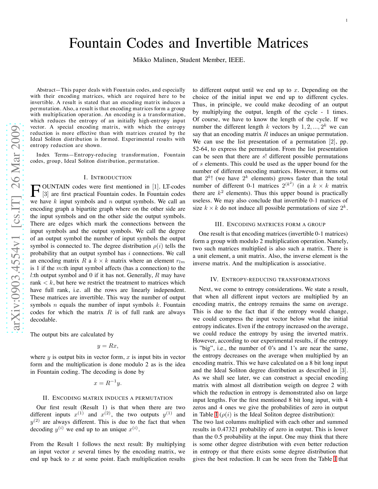
The two last columns multiplied with each other and summed results in 0.47321 probability of zero in output. This is lower than the 0.5 probability at the input. One may think that there is some other degree distribution with even better reduction in entropy or that there exists some degree distribution that gives the best reduction. It can be seen from the Table I Fig. 1. Saving in bits (vertical direction) when transformation is applied to input of length 30204 with different reduced number of ones in the input (horizontal direction) degree i = 2 gives the lowest probability of zero in the output, 0.42857. We used this degree and formed a special invertible encoding matrix R:

For example, a 4 × 4 encoding matrix R would be:

There is a single 1 in the last row at the last column. These matrices are invertible and thus suitable for encoding and decoding. We ran simulations

…(Full text truncated)…

This content is AI-processed based on ArXiv data.