Supernodal Analysis Revisited

In this paper we show how to extend the known algorithm of nodal analysis in such a way that, in the case of circuits without nullors and controlled sources (but allowing for both, independent current and voltage sources), the system of nodal equations describing the circuit is partitioned into one part, where the nodal variables are explicitly given as linear combinations of the voltage sources and the voltages of certain reference nodes, and another, which contains the node variables of these reference nodes only and which moreover can be read off directly from the given circuit. Neither do we need preparational graph transformations, nor do we need to introduce additional current variables (as in MNA). Thus this algorithm is more accessible to students, and consequently more suitable for classroom presentations.

💡 Research Summary

The paper revisits the classic Supernodal Analysis (SNA) technique for linear circuits and proposes a streamlined algorithm that can be taught easily to undergraduate students. Traditional Nodal Analysis (NA) works well for circuits that contain only admittances and independent current sources, because the node‑admittance matrix Yₙ and current vector Jₙ can be read directly from the schematic. However, as soon as independent voltage sources, controlled sources, or nullors appear, NA must be extended. The Modified Nodal Analysis (MNA) solves the general case by introducing extra current variables for voltage sources, but its matrix formulation is considered too abstract for introductory courses.

The author therefore refines the definition of a “supernode”: a maximal connected sub‑circuit consisting solely of nodes and independent voltage sources. Under this definition, an ordinary node that is not incident to any voltage source is itself a supernode. Each supernode is assigned a local reference node (the global reference node 0 may serve as a local reference for its own supernode). The key insight is that, if every supernode has a tree topology (or, more generally, if any loop of voltage sources inside a supernode satisfies Kirchhoff’s Voltage Law), then the voltage of any node inside the supernode can be expressed uniquely as the voltage of its local reference plus the signed sum of the voltage sources that lie on the unique path from the reference to the node.

The algorithm proceeds in four steps:

1. Initialization – Identify all supernodes, count the number N + 1 of nodes after contracting each supernode to a single vertex, and choose local reference nodes.
2. Express internal voltages – For each supernode, write every internal node voltage as a linear combination of the local reference voltage and the independent voltage sources belonging to that supernode.
3. Apply KCL at supernodes – Write one Kirchhoff‑Current‑Law equation per supernode (except the one containing the global reference). Because the internal voltages have already been eliminated, each equation involves only the local reference voltages.
4. (Optional) Handle controlled sources – Temporarily treat voltage‑controlled sources as independent voltage sources (“taping”), apply the same procedure, and finally substitute the controlling variables back (“untaping”).

After step 3 the system of equations has the compact form

  bYₙ · bVₙ = bJₙ

where bVₙ is the vector of local‑reference node voltages, bYₙ is the node‑admittance matrix of the contracted circuit (the graph obtained by collapsing each supernode to a single node and removing loops), and bJₙ is a current vector that accounts for independent current sources and the contribution of voltage sources.

The major contribution of the paper is a pair of “fill‑in” rules that allow bYₙ and bJₙ to be read directly from the original schematic without any graph transformations or extra algebra:

• Rule 1 (bYₙ entries) – The diagonal entry (A,A) equals the sum of all admittances that are incident on supernode A at exactly one end. The off‑diagonal entry (A,B) equals the negative of the sum of all admittances that connect supernodes A and B. Admittances that touch the same supernode at both ends are ignored because they cancel out in KCL.

• Rule 2 (bJₙ entries) – For each supernode A (excluding the datum node), the corresponding entry of bJₙ is obtained by:

  • Adding the currents of all independent current sources directed into A,
  • Subtracting the currents of all independent current sources directed out of A,
  • Adding, for each admittance Gₖ that connects A to another supernode, the product Gₖ · Σ_Aₖ, where Σ_Aₖ is the signed sum of the voltages of all independent voltage sources lying on the unique oriented path γ_A_Gₖ that starts at the local reference of the opposite supernode, traverses the admittance Gₖ, and ends at the local reference of A. The sign of each voltage source in Σ_Aₖ is positive if the source polarity opposes the path orientation, negative otherwise.

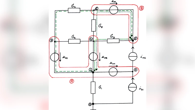
These rules are illustrated with a small example circuit containing two voltage sources, several resistors, and a current source. The paper shows how the supernodes are identified, how internal node voltages are expressed, and how the reduced 2 × 2 system (equation (2) in the text) is obtained directly from the schematic using the two rules.

The author also discusses extensions:

• Voltage‑controlled current sources (VCCS) – By treating the controlling voltage source as an independent source during the supernode construction, the same rules apply. After solving the reduced system, the controlling voltage is substituted back.
• Current‑controlled sources (CCCS) – Currents that belong to branches inside a supernode can be expressed as sums of currents entering the supernode through its leaf nodes (in a rooted‑tree view). KCL at the root then yields the required expressions.
• Nullors – The paper attempts to apply the same methodology to circuits containing nullors but concludes that the supernode concept becomes contradictory: nullors both fix node voltages (through the nullator) and require those voltages to appear as variables (through the norator). Consequently, no simple fill‑in rule analogous to Rules 1 and 2 can be derived for nullor‑containing circuits, and this remains an open problem.

In summary, the paper delivers a pedagogically friendly version of Supernodal Analysis that avoids the extra variables and graph‑theoretic preprocessing required by MNA. By providing explicit, diagram‑based rules for constructing the reduced admittance matrix and source vector, it makes the method accessible to students and suitable for classroom demonstration, while still being rigorous enough for practical circuit analysis. The limitations concerning controlled sources and nullors are clearly identified, pointing to directions for future research.