On the Iterative Decoding of High-Rate LDPC Codes With Applications in Compressed Sensing

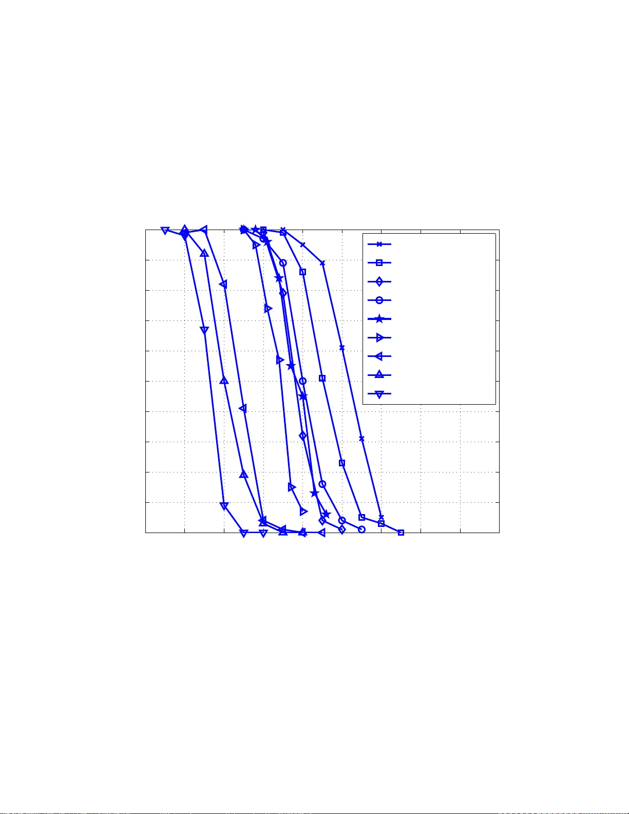
1 V eriﬁcat ion Decoding of High-Rate LDPC Codes with Applications in Compressed Sensing (CLN 9-610 First Re vision 01/22/12) Fan Zh ang a nd Henry D. Pﬁster Departmen t of E lectrical an d Com puter En gineerin g, T exas A&M University {fanzhang, hpﬁster}@tamu.ed u Abstract This paper considers the performance of ( j, k ) -regular lo w-density parity-check (LDPC) codes with message- passing (MP) dec oding algorithms in the high-rate r egime. In particular, we deriv e the high-rate scaling law for MP decoding of LDPC codes on the binary erasure channel (BE C) and the q -ary symmetric channel ( q -SC). For the BEC and a ﬁxed j , the density evo lution (DE) threshold of iterative decoding scales like Θ( k − 1 ) and the cri tical stopping ratio scales like Θ( k − j / ( j − 2) ) . For the q -SC and a ﬁxed j , the DE threshold of veriﬁcation decoding depends on the details of the decoder and scales like Θ( k − 1 ) for one decoder . Using the fact t hat coding ov er large ﬁnite alphabets is very similar t o coding over the real numbers, the analysis of veriﬁcation decoding is also extended to the the compressed sensing (CS) of strictl y-sparse signals. A DE based approach is used to analyze t he CS systems with randomized-reco nstruction guarantees. This leads t o the result that strictly-sparse signals can be r econstructed ef ﬁciently with high-probability using a constant oversamp ling ratio (i .e., when the number of measurements scales linearly with the sparsity of the signal). A stopping-set based approach is also used to get stronger (e.g., uniform-in-probability) reconstruction guarantees. Index T erms LDPC codes, veriﬁcation decoding, compressed sensing, stopping sets, q -ary symmetric channel I . I N T RO D U C T I O N Compressed sensing ( CS) is a relativ ely n ew area o f sign al proce ssing th at has re cently received a large amount of atten tion. Th e main idea is that many real-world sig nals ( e.g., those sparse in so me transform d omain) can be reconstruc ted from a relativ ely small n umber of lin ear m easurements. I ts r oots lie in th e areas o f statistics and signal processing [1], [2], [3], but it is also very much r elated to p revious work in co mputer science [4], [5] and applied mathematics [6], [7], [8] . CS is also very closely r elated to error corre cting code s, a nd ca n be seen as source codin g using linear co des over rea l n umber s [9], [1 0], [1 1], [12], [ 13], [1 4], [1 5]. October 24, 2018 DRAFT 2 In this paper, we analyze the perform ance o f low-density p arity-che ck ( LDPC) codes with veriﬁcation d ecoding [16] as applied to CS. The resultin g appr oach is alm ost ide ntical to that o f Sudo codes [9], but ou r n ew perspective allows one to numer ically comp ute sparsity thr esholds for a broa d class of m easurement matrices un der veriﬁcation - based decod ing. Changing the en semble of measuremen t matrices also allows an unbo unded reduction in th e oversampling ratio relative to Sudoco des. A scaling ap proach is ado pted to d erive simple expressions for the sp arsity threshold as it appro aches zero . Since ma ny interesting application s of CS in volve very sparse (or com pressible) signals, this is a very inter esting regime. From a c oding per spectiv e, this correspo nds to the high -rate limit and our results also have imp lications for veriﬁcation- based decodin g o f LDPC codes over large ﬁn ite ﬁelds. The analy sis o f CS in this p aper is based on the noiseless measu rement o f strictly -sparse signals [6], [3], [9]. In the real world, the measuremen t process may introd uce noise and reco nstruction algo rithms m ust be im plemented with ﬁnite-precision arithmetic. Altho ugh the veriﬁcation deco der discussed in this paper is un stable in the pr esence of n oise, this does not imp ly that its perform ance an alysis is not useful. Th e veriﬁcation dec oder can be seen as a suboptimal version of list-message p assing decoder [17], wh ich itself can be seen as a high-SNR limit o f the fu ll belief-pr opagation (BP) decod er fo r CS [10], [11]. Idea lly , o ne would study the BP d ecoder directly , but the DE analysis techniq ue remains intra ctable for dec oders that pass fun ctions as messages. Still, we expect that a su ccessful analysis of the BP d ecoder would show that its perfor mance is lower bound ed by the veriﬁcation decoder . Sparse me asurement m atrices and message-p assing r econstructio n algorithms fo r CS wer e intro duced in [9], [10]. Both ideas h av e since been considered by a n umber o f o ther au thors [ 12], [1 3], [1 8], [19], [20], [21], [ 22], [23], [24]. For example, [19], [1 8] show empirically that spar se binary measur ement matrices with linear-programm ing (LP) r econstruction are as goo d as den se rand om matrices. In [22], [23], d ense m atrices with i.i.d. Gaussian random entries and an itera ti ve threshold ing alg orithm, which is a message- passing ty pe of algorithm , is proved to h av e the same spar sity-under sampling trad eoff as co n vex o ptimization reco nstruction. In [20], sparse measureme nt m atrices and me ssage-passing deco der ar e u sed to solve a sparse signal recovery prob lem in the ap plication of per-ﬂo w data measuremen t on high-sp eed link s. All these works imp ly that sparse matrices with message-p assing reconstructio n algorithm s can be a g ood solu tion for CS systems. For reconstru ction, the minimu m numbe r of measureme nts d epends on the signa l model, the measureme nt noise, the recon struction algorithm, and the way rec onstruction error is measur ed. Consider the reconstru ction of a length - n signal that ha s p no n-zero (or do minant) entries. For strictly-sparse sign als, Dono ho comp uted sparsity thr esholds below which LP r econstructio n su cceeds w .h. p. f or h igh-dim ensional signals [25], [26]. For a comp ressible sign al with noisy m easuremen ts, [27] deri ves an informatio n-theore tic bound th at shows Ω ( p ln( n/p )) noisy measurem ents are requ ired. In [ 28], it is shown that O ( p ln( n/p )) no isy m easurements a re needed to reconstruct a strictly-sparse signal. In [29], it is shown that the lower bound O ( p ln( n/p )) canno t be furthe r imp roved (r educed) fo r a certain compressible sig nal model. In this paper, we sh ow th at veriﬁcation-based reco nstruction allows line ar-time (in the signal dimen sion) recon struction of strictly -sparse signals with O ( p ) mea surements u sing r eal-valued measuremen t matrices and noiseless measurements. At ﬁrst, this seems to vio late the lo wer bo unds on the number of measurements. Howe ver , we provide a inform ation-theo retic explanation th at shows the O ( p ln( n/p )) lower bound d oes not apply October 24, 2018 DRAFT 3 to this system because the measurem ents are real-valued an d provid e an inﬁnite amoun t of infor mation when ther e is n o measureme nt n oise. A. Main Contribution This p aper provid es detailed description s and extension s of work r eported in two co nferenc e pap ers [13], [14]. W e b eliev e the main contribution of all these results are: 1) The ob servation th at th e Sudoco des reconstru ction algorith m is an instance of veriﬁcation decod ing and its decodin g thresho lds can b e co mputed precisely using num erical DE [13]. For en sembles with at least 3 non- zero en tries in each colu mn, this implies th at n o o uter co de is requ ired. For signals with δ n non- zero entries, this reduces the lower b ound on th e nu mber o f no iseless me asurements req uired f rom O ( n ln n ) to O ( n ) . 2) The introduction of the high-rate scaling analysis for iterativ e erasure and veriﬁcation decoding of LDPC codes [13], [14]. This tech nique provide s closed-for m upp er an d lower bou nds on deco ding th resholds that hold unifor mly as the ra te appr oaches 1. For example, it shows th at (3 , k ) -LDPC co des achieve 8 1% of capacity on the BEC for sufﬁciently large k . Th is also shows that, fo r strictly-sparse signals with δ n non -zero en tries and noiseless measurem ents, 3 δ n measuremen ts are sufﬁcient (with (4 , k ) -L DPC codes) for veriﬁcation- based r econstructio n u niformly as δ → 0 . While it is known that δ n + 1 measur ements are sufﬁcient for reconstruc tion v ia exhaustive search of all support sets [30], th is shows th at O ( δ n ) measuremen ts a lso sufﬁce for sparse m easurement matr ices with low-complexity rec onstruction . In constrast, the best bou nds for linear- progr amming reconstruc tion require a t le ast O  δ n ln 1 δ  measuremen ts. 3) The application of the high -rate scaling analysis to com pute the stopping distance of erasure and veriﬁcation decodin g. For example, this shows that almost all lo ng ( j, k ) -LDPC codes, with j = 2 + ⌈ 2 ln( k − 1 ) ⌉ , can correct all erasure patter ns who se fra ction o f er asures is smaller than 1 k − 1 . B. Structu r e of the P aper Section II provid es background information on coding and CS. Section II I summar izes the main results. In Section IV, proofs and details are giv en for the main results based on DE. W hile in Section V, proof s an d details are provided for the main r esults based on stoppin g-set an alysis. Section VI d iscusses a simple inf ormation -theoretic bound on the number o f m easurements re quired f or r econstructio n. Sec tion VII p resents simulatio n r esults co mparing the algorithm s d iscussed in this paper with a ran ge of other algo rithms. Finally , some co nclusions are discussed in Section VIII. [Author ’ s Note: T he eq uations in this paper were orig inally typeset for two-co lumn p resentation, but we have submitted it in one- column forma t for easier readin g. Please acce pt our ap ologies f or some of the rough looking equations.] October 24, 2018 DRAFT 4 I I . B AC K G RO U N D O N C O D I N G A N D C S A. Backgr ound on LDPC Codes LDPC co des are linear co des introdu ced by Gallager in 1962 [3 1] and re-discovered b y MacKay in 199 5 [3 2]. Binary LDPC cod es are now known to b e capacity app roaching on various ch annels when the b lock length ten ds to inﬁnity . They can b e rep resented by a T anner graph , where the i -th variable no de is co nnected to the j -th check node if th e entry on the i -th colu mn and j -th row of its parity-ch eck matrix is n on-zero . LDPC co des can be deco ded by an iterative message-passing (MP) algorithm, wh ich passes m essages between the variable nodes and ch eck no des iterativ ely . If the messages passed a long th e e dges are probab ilities, th en the algorithm is also called b elief pr opagation (BP) decod ing. T he p erform ance of the MP alg orithm can b e ev aluated using d ensity evolution (DE) [3 3] and stoppin g set (SS) analysis [3 4] [3 5]. Th ese techniq ues allow one to c ompute noise th resholds (b elow which decod ing succeeds w . h.p.) for average-case and worst-ca se erro r mod els, respectively . B. Enco ding and Decod ing An LDPC code is deﬁned by its parity-check matrix Φ , which can be represen ted by a sparse bipartite graph . In the bipartite graph , there are two types of nod es: v ariable nodes repre senting code symbols and check no des representing parity-ch eck equ ations. In the standard irregular cod e ensemble [ 36], the co nnections between variable nod es a nd check n odes are d eﬁned by the degree distribution (d. d.) pairs λ ( x ) = P d v i =1 λ i x i − 1 and ρ ( x ) = P d c i =1 ρ i x i − 1 where d v and d c are the maxim um variable and check n ode degrees an d λ i and ρ i denote the fractio n of edges co nnected to degree- i variable and chec k n odes, respectively . The sparse grap h r epresentation of LDPC cod es imp lies th at the en coding and decoding algo rithms can be implem ented with linear com plexity in th e blo ck length 1 . Since LDPC cod es are usually deﬁned over the ﬁnite ﬁeld GF ( q ) instead of the real numb ers, we need to m odify the encodin g/decodin g algorithm to d eal with sign als over r eal nu mbers. Eac h en try in the p arity-check m atrix is chosen either to be 0 or to be a real number drawn from a contin uous d istribution. The par ity-check matrix Φ ∈ R m × n can also be used as the mea surement matrix in the CS system (e.g., th e signal vector x ∈ R n is o bserved as y = Φ x ); if there are no degree- 1 nod es, then it will be f ull-rank with hig h p robability (w .h.p.). The process of gen erating th e measu rement variables can also be seen fr om the b ipartite T anner graph repre- sentation. Figure 1 shows the en coder stru cture. Each no n-zero entry in Φ is the edge- weight of its correspon ding edge in this gr aph. Th erefore, the me asurement p rocess associate d with a degree d ch eck node is as fo llows: 1) Encoding: Th e measurement variable is the weighted sum (using the edge weights) of the d neighbor ing variable nodes giv en by y i = P j Φ ij x i . In this work, we con sider only strictly-sp arse signals a nd we use two deco ders based on veriﬁcatio n, wh ich wer e ﬁrst pro posed and an alyzed in [ 16]. Th e second algorithm was also p roposed inde penden tly f or CS in [9]. The decodin g p rocess u ses th e following rules: 1 The complexity here refers to both the time and s pace complexi ty in terms of basic ﬁeld operations and storage of ﬁeld elements, respecti ve ly . October 24, 2018 DRAFT 5 Figure 1. Structure of the encode r . 1) If a measurem ent is zero, then all n eighbo ring variable nodes are veriﬁed as zero. 2) If a check node is of degree one, then verify the variable no de with the value of the measurem ent. 3) [Enhanced veriﬁcation] If two check n odes overlap in a single variable nod e a nd have the same measur ement value, then verify that variable no de to the value of the measureme nt. 4) Remov e all veriﬁed variable nod es an d the edges attach ed to them by subtracting out the veriﬁed values from the measureme nts. 5) Repeat steps 1-4 until decod ing succeeds or m akes no fu rther pr ogress. Note the ﬁrst alg orithm follows steps 1, 2 , 4 and 5. T he second algorith m fo llows steps from 1 to 5. These two algorithm s correspon d to the ﬁrst and seco nd algorithms in [ 16] an d ar e referred to as L M1 an d n ode-b ased L M2 (LM2-NB) in th is p aper 2 . Th e Sud ocodes intr oduced in [9] are simply LDPC codes with a r egular check d.d. and Poisson variable d .d. that u se LM2-NB reco nstruction . On e d rawback of this choice is that th e Poisson v ariable d.d. with ﬁnite- mean h as (w .h .p.) a linear fraction of variables nodes that do n ot particip ate in any measur ement [38]. For this reason , Sudoc odes req uire a two-ph ase enc oding that prevents the sche me from ach ieving a con stant oversampling rate. A detailed discussion of the LM2-NB algo rithm, which is a n ode-based imp rovement of th e message-based LM2 ( LM2-MB), ca n b e found in [1 7]. In gene ral, th e scheme de scribed above does no t guarante e that all veriﬁed symbols ar e actually co rrect. The ev ent th at a symb ol is veriﬁed but inco rrect is called false veriﬁcation (FV). In o rder to guaran tee there ar e no FVs, one can ad d a constraint on the signal such that th e weigh ted sum, of any subset of a che ck nod e’ s non -zero neighbo rs, does no t equal to zero [9], [12]. Another scenar io wh ere it makes sense to assume no FV is when we consider rando m signals with co ntinuou s distributions so that FV occurs with prob ability zero. Finally , if th e measured sig nal is a ssumed to be no n-negative, then FV is impossible for the LM1 d ecoding algorithm. V eriﬁcation d ecoding was or iginally introd uced and analyze d for the q -SC. It is based on the obser vation tha t, over large alphabets, the probab ility that “two indepen dent random n umbers are equ al” is quite small. This lead s 2 In [16], the second algorithm (which we refer to as LM2) was describe d in a node-based (NB) fashion (as abov e), but analyzed using a message-based (MB) density-e vol ution. There is an implici t assumption that the two algorithms perform the same. In fact, they perform dif ferent ly and the LM2-NB algorith m is superior as observ ed in [37][17]. October 24, 2018 DRAFT 6 to th e veriﬁcation assumption that any two m atching values ( during de coding) ar e gen erated by the same set of non-ze ro c oefﬁcients with high p robab ility . The primary connection between CS, codes over real numbers, a nd veriﬁcation deco ding lies in the fact th at: The veriﬁcation assumption a pplies eq ually well to b oth larg e discr ete alp habets and the r eal n umbers. C. An alysis T o ols Based on the sparse grap h structure, LDPC codes can be decoded efﬁciently u sing iterative MP algorithms. The average per forman ce of MP decodin g algo rithms ca n be analy zed with density ev olution (DE) [33] o r extrinsic informa tion transfer (EXI T) char ts [39]. Th e co ncentration the orem [3 3] shows th at ran dom r ealizations o f d ecoding are close to the av erage be havior w .h .p. fo r lon g b lock leng ths. DE analysis provides a thresho ld below which decodin g (or rec onstruction ) suc ceeds w .h. p. as the blo ck le ngth goes to inﬁn ity . The decod ing thre shold can also be im proved b y o ptimizing th e edge degree distribution (d. d.) pair λ ( x ) and ρ ( x ) . Decoding can also be analyzed using combinator ial metho ds such as stopping-set analysis [3 4] and [35]. Stopping- set a nalysis gives a threshold b elow which all error pattern s can b e recovered with ce rtainty un der the assum ption of no FV . In ge neral, DE and stopping-set analysis lead to different thr esholds. Since stoppin g-set analy sis implies unifor m recovery o f all the error patterns, instead of just m ost of them , th e thresho ld given b y stopping -set a nalysis is always lower than the one given by DE. For example, DE analy sis of (3 , 6 ) regular co des o n the BEC shows that almost all erasu re p atterns o f size less than 0 . 4 29 of the block leng th c an b e corrected w .h .p. [36]. On th e other hand, stoppin g-set an alysis guarantees th at most code s corr ect all e rasure patterns of size less th an 0 . 018 of the block len gth as n → ∞ . Like wise, in CS systems, there are two stand ard measure s of r econstructio n: un iform r econstructio n an d random- ized (or no n-uniform ) recon struction. A CS system ach iev es r andomize d re construction for signal set (e.g., p -spar se signals) if most rand omly ch osen m easuremen t matrices recover most of the sign als in the signal set. While a CS system ach iev es unifor m reconstructio n if a measu rement matrix an d the deco der recover all the sign als in the sign al set w ith certainty . Ano ther criterio n, which is between unifo rm reco nstruction and rando mized recon struction, is what we call uniform-in- pr o bability reco nstruction. A CS system achieves uniform -in-pro bability rec onstruction if, for any signal in the signal set, most rand omly chosen measurem ent matrices achieve successfu l deco ding. Since DE and th e co ncentration theore m lead to w .h. p. statements fo r MP d ecoding over all signals and graph s, it is natu ral to adopt a DE ana lysis to evaluate the p erform ance o f rand omized reconstru ction CS systems b ased on LDPC codes. For u niform r econstructio n, a stopping -set analysis of the MP decod er is the natu ral choice. Wh ile this works for the BEC, the p ossibility of FV prevents th is type of strong statement for veriﬁcation d ecoding . If the n on-zero entries of Φ are c hosen ran domly from a continuo us distribution, howev er , then the probability of FV is zero for all signa ls. T herefor e, one can use stopp ing-set an alysis to analyze MP deco ding of LD PC co de ensembles and show that the LDPC codes with M P deco ding ach iev es u niform- in-pro bability reconstruction for the CS system . The reader is caution ed that these results are somewhat brittle, howev er , be cause they rely on exact calculation an d m easuremen t of r eal number s. October 24, 2018 DRAFT 7 While the method s d iscussed above can be used to num erically c ompute sparsity threshold s o f veriﬁcation-b ased reconstruc tion fo r irregular LDPC-type measur ement matrices, we are par ticularly interested in und erstanding h ow the num ber o f measurem ents scales w hen the signal is b oth high-d imensional and extrem ely spar se. T o compar e results, we focu s o n the oversampling r atio (i.e., the n umber of measuremen ts d i vided by the numb er of non- zero elements in th e signal) required for reconstructio n. This leads us to consider the high-rate scaling of DE and stopping- set analysis. D. Decod ing Algo rithms In CS, optim al decodin g (in te rms o f oversampling ratio) req uires a com binatorial search that is known to be NP-Hard [40]. Practical reconstru ction algo rithms ten d to either b e based o n linear prog ramming (e. g., b asis pu rsuit (BP) [1]) or low-complexity iter ati ve algorithm s (e.g ., Ortho gonal Matching Pursuit (OMP) [4 1]). A wide ran ge of a lgorithms allow one to trade- off the oversampling ratio for recon struction co mplexity . In [9], LDPC codes are used in the CS system and th e algorithm is essentially identical to the veriﬁcation- based decodin g prop osed in [16]. The scaling -law analysis shows the oversampling ratio for LDPC cod es based CS system can be quite good. Encodin g/decod ing comp lexity is also a consideratio n. LDPC codes have a sparse bipartite-g raph repr esentation so that encodin g a nd decoding is p ossible with co mplexity linear in the blo ck len gth. There are se veral existing MP decod ing algorith ms fo r LDPC co des over no n-bina ry ﬁelds. I n [36] and [42], an analysis is intr oduced to ﬁnd provably capacity-ac hieving co des f or erasur e ch annels under MP de coding. Metz ner presents a mod iﬁed m ajority-log ic decod er in [ 43] that is similar to veriﬁcation deco ding. Davey and MacKa y develop and ana lyze a symb ol-level MP decoder over small ﬁnite ﬁelds [4 4]. T wo veriﬁcatio n deco ding algor ithms for large discrete alph abets are pro posed by Lu by and Mitzenm acher in [ 16] an d ar e called LM1 and LM 2 in this paper . The list-m essage-passing (LMP) algo rithm [17] pr ovides a smooth trade- off between the pe rforman ce and complexity of the two d ecoding algorithms introduc ed by Shokr ollahi an d W ang in [4 5]. All of these algor ithms are sum marized in [ 17]. One can get a rough idea o f the perfo rmance of th ese a lgorithms b y co mparing their perform ance for the standard (3 , 6) -regular LDPC co de. A standard pe rforman ce measu re is th e noise threshold (o r sparsity th reshold for CS) below which de coding succ eeds with high prob ability . The threshold of the LM1 algorith m in this case is 0 . 16 9 . This means that a long r andom (3 , 6) -regu lar LDPC code will corr ect a q -SC erro r p attern with high pro bability as long as the er ror r ate is less than 0 . 1 69 . Like wise, it means that u sing the sam e code for LM1 r econstruction of a strictly- sparse signal will succeed w .h.p. as long as th e spar sity rate (i.e., fraction of non-ze ro elements) of the sign al vector is less than 0 . 169 . The LM2 -MB algorith m im proves this thresho ld to 0 . 210 an d the LM2-NB algorithm is co njectured to imp rove th is th reshold to 0 . 25 9 [ 17]. Like wise, the stopping -set an alysis of the LM1 algorithm in Section V shows that a (3 , 6) -regular code exists where LM1 suc ceeds (ig noring FV) for a ll er ror (or sparsity) p atterns wh ose frac tion o f no n-zero entr ies is less than 0 . 0055 . In co mparison, th e BEC stoppin g-set threshold of the (3 , 6) code is 0 . 0 1 8 fo r erasur e pattern s. Howe ver , both of these thresho lds can be incre ased sign iﬁcantly (fo r the same code rate) by incre asing the variable no de October 24, 2018 DRAFT 8 0 0.1 0.2 0.3 0.4 0.5 0.6 0.7 0.8 0.9 0 0.05 0.1 0.15 0.2 0.25 0.3 0.35 1−rate Error Threshold LM1SS BECSS LM1DE Figure 2. Thresholds vs 1- R , where R is the code rate, for L M1 stopping s et/DE analysis and the BEC stopping-set analysis. degree. In fact, th e (7 , 14) -regular LDPC co de gives the b est (bo th LM1 an d BEC) stopping-set thresho lds and they are (respec ti vely) 0 . 0364 and 0 . 0 645 . Finally , if th e signal is non -negativ e, then FV is not possible dur ing LM1 de coding and th erefore 0 . 03 6 4 is a lower b ound on the tru e LM1 rate- 1 2 threshold for uniform recon struction. Fig. 2 shows the best decoding /recovery th resholds fo r regu lar LD PC co des with BEC stopping-set analy sis, LM1 stopping- set analysis, LM1 DE analysis LM2-MB DE analysis and the boun d by using linear progr amming (LP) decodin g with dense measure ment matrix [21]. As we can see from Fig. 2 , LM2- MB DE gives the b etter upp er bound in the high- rate regime. Note th at if the signal coefﬁcients are non -negative, the thre shold of LM1 given by stopping- set a nalysis is co mparab le to th e stro ng b ound given in [ 46, Fig . 1 (a)], and th e thresho ld of LM1 given by DE analysis is co mparab le to the weak bo und given in [ 46, Fig. 1( b)]. Since the scaling-law a nalysis becom es so mewhat tediou s wh en com plicated algorithms are applied, we co nsider only the ( j, k ) -regular cod e en semble an d the relatively simple alg orithms LM1 and LM2- MB. The rathe r surp rising result is that, even with regular c odes and simple decodin g algo rithms, th e scalin g law imp lies that LDPC codes with veriﬁcation deco ding perfo rm very well fo r n oiseless CS systems with strictly-spar se signals. E. Sign al Model There are some signiﬁcant differences b etween coding theo ry a nd CS. On e of them is the signal mo del. The ﬁrst d ifference is that co ding the ory typ ically uses d iscrete alph abets (see [47] f or one exception to th is) while CS deals with signals over th e real numb ers. Fortunately , some codes design ed for large discrete alph abets ( e.g., the q -ary symmetric channel) can be a dapted to the real num bers. By explor ing the c onnection an d th e an alogy between real ﬁeld and ﬁnite ﬁeld with large q , the CS system can be seen as an essentially a syn drome -based source co ding system [13]. Usin g the par ity-check matrix o f a n on-bin ary LDPC co de as th e measureme nt matrix , the MP decodin g alg orithm ca n b e used as the rec onstruction algo rithm. The second difference in the signal mod el is that CS u sually models the sparse sig nal x ∈ R n as coming from a October 24, 2018 DRAFT 9 particular set, such as th e n -dim ensional unit ℓ r -ball. This co nstraint enfo rces an “ap proxima te sparsity” p roperty of the signal. In informatio n theo ry and cod ing, th e signal model is typically pro babilistic. Each compo nent o f the signal is d rawn i.i. d. from a distribution, on the real n umbers, that d eﬁnes the sign al ensemble. A strictly- sparse signal ca n be ca ptured in this pro babilistic mode l by choo sing the distribution to contain a Dirac delta func tion at zero [10], [ 21], [ 11]. F . Inter esting Rate Re gime In coding th eory , the cod e r ate d epends on the app lication and the interesting rate regime varies fro m close to zero to almost o ne. In CS sy stems, the signal is spar se in so me d omain and becomes in creasingly sparse as th e dimension incr eases. In tuitiv ely , this m eans that on e can use cod es with very little r edund ancy or very h igh cod e rate to r epresent th e sign al. The setting where CS systems achieve th e largest gains co rrespond s to the hig h-rate regime in codin g. Therefor e, we con sider how the system p arameters must scale as the rate g oes to one . It is imp ortant to note that the re sults p rovide bound s for a wide range o f r ates, but are tight as the r ate app roaches o ne. I I I . M A I N R E S U LT S The main m athematical results of this p aper ar e now listed. Details and pro ofs follow in section IV an d section V. Note that all results hold for a symptotically- long rando mly-cho sen regular LDPC codes with variable-degree j and check- degree k . Th e m ain idea is to ﬁx j and ob serve how th e decoding threshold scales when increase k . This provides a scaling law fo r the d ecdoing thresho ld a nd leads to nec essary a nd sufﬁcient co nditions for successful reconstruc tion. (i) [DE- BEC] For the BEC, ther e is a K < ∞ such that: a chec k-regular LDPC code with average variable n ode degree j ≥ 2 and che ck-degree k can recover a δ < ¯ αj / ( k − 1) fraction of erasu res (w .h .p. as n → ∞ ) when k ≥ K . Th e constant ¯ α is in depend ent of k and gives the f raction of the optimal δ ∗ = j /k th reshold. Con versely , if the er asure p robab ility δ > ¯ αj / ( k − 1) , then decod ing fails (w .h.p . a s n → ∞ ) fo r all k . (ii) [ SS-BEC] For any 0 ≤ θ < 1 , there is a K < ∞ such that: fo r all k ≥ K , a ( j, k ) -regula r LDPC code with j ≥ 3 can recover all erasur es (w .h.p. as n → ∞ ) of size θ ne ( k − 1 ) − j / ( j − 2) . (iii) [DE- q -SC-LM1] For the q -SC, when one cho oses a code ran domly f rom the ( j, k ) regular ensemble with j ≥ 2 and uses LM1 as decoding algorithm, then there is a K 1 < ∞ such that one can recover alm ost all error patterns of size nδ fo r δ < ¯ α j ( k − 1) − j / ( j − 1) (w .h. p. as n → ∞ ) for all k ≥ K 1 . Con versely , when δ > ¯ α j ( k − 1) − j / ( j − 1) , there is a K 2 < ∞ such that the decoder fails (w .h.p. as n → ∞ ) for all k ≥ K 2 . (iv) [DE- q -SC-LM2-MB] For the q -SC, wh en o ne chooses a co de r andomly fr om the ( j, k ) regular ensemble with j ≥ 3 an d uses LM2-M B as d ecoding alg orithm, th en ther e is a K 1 < ∞ such tha t on e can recover almost all error pa tterns of size nδ f or δ < ¯ α j j /k ( w .h.p . as n → ∞ ). The constant ¯ α j is in depend ent of k a nd giv es the fraction of the optimal δ ∗ = j /k threshold. Co n versely , there is a K 2 < ∞ such tha t the decod er fails (w . h.p. as n → ∞ ) w hen δ > ¯ α j j /k for all k ≥ K 2 . October 24, 2018 DRAFT 10 (v) [SS- q -SC-LM 1] For any 0 ≤ θ < 1 , th ere is a K < ∞ such that: For all k ≥ K , a ( j, k ) -r egular LDPC cod e with j ≥ 3 u sing LM1 d ecoding can recover ( w .h.p as n → ∞ ) all q - SC erro r patterns of size θn ¯ β j ( k − 1) − j / ( j − 2) if no false veriﬁcations o ccur . For the sake of simplicity an d unif ormity , the c onstants K , K 1 , K 2 and ¯ α j are reused even thoug h they may take d ifferent values in (i) , (ii), ( iii), (iv) an d ( v). I V . H I G H - R A T E S C A L I N G V I A D E N S I T Y E VO L U T I O N A. DE Sca ling-Law An alysis for the BEC DE analysis provides a n explicit recur sion, wh ich conn ects th e distributions of me ssages passed fro m variable nodes to check nod es at two consecutive iterations of MP algorithm s. In the ca se o f BEC, this DE ana lysis ha s b een derived in [48] and [ 36]. It has been sh own th at the expected f raction o f erasur e messages, which a re p assed in the i -th iteration, called x i , evolves a s x i = δ λ (1 − ρ (1 − x i − 1 )) w here δ is the erasure probab ility of the c hannel. For general chan nels, the recu rsion may be much mo re complicated beca use one h as to trac k the gen eral distributions, which cannot b e represented by a single para meter [49]. T o illustrate th e scalin g law , we start by analyzin g the BEC case using DE . Alth ough this is not applicab le to CS, it motiv ates th e scaling-law analysis for the q -SC, which is related to CS. The scaling law of LDPC codes of check-regular ensemble over the BEC is shown b y th e following theo rem. Theorem 1. Consider a sequen ce of check-r e gular LDPC codes with ﬁxed variable d e gr ee distribution λ ( x ) and incr easing chec k de gr ee k . Let j = 1 / ´ 1 0 λ ( x ) d x be the a verage variable degr ee and α , which is called α - thr eshold, be the lar gest α such tha t λ  1 − e − αj x  ≤ x for x ∈ [0 , 1] . F or the erasure pr obability δ = αj / ( k − 1) , the iterative d ecoding of a rando mly chosen len gth- n co de fr om this ensemble fails (w .h. p as n → ∞ ) for a ll k if α > α . Conver sely , if α < α , then th er e exists a K < ∞ such tha t iterative decodin g succeeds (w .h.p a s n → ∞ ) for all k ≥ K . Before pr oceeding to the p roof of T heorem 1, we introd uce two lemmas that will be u sed throu ghout the p aper . Lemma 2 . F or all s ≥ 0 , x ≥ 0 an d k 1+ s > | x | , the seque nce a k =  1 − x k 1+ s  k is strictly in cr easing in k and 1 − xk − s ≤ a k ≤ e − xk − s . (1) Pr o of o f Lemma 2: W e r estrict ou r attention to x ≥ 0 b ecause the proo f is simp liﬁed in this case an d th e continuatio n does no t require x < 0 . W e show that a k is strictly increasing with k by con sidering the p ower series expansion of ln a k , which con verges if k 1+ s > | x | . This gives ln a k = k ln  1 − x k 1+ s  = − xk − s − ∞ X i =2 x i i k (1+ s ) i − 1 , (2) and keeping only the ﬁr st te rm shows th at ln a k ≤ − xk − s . Since all the ter ms are negative an d decreasing with k , we see that a k is strictly increasing with k . Since a k is conv ex in x for k 1+ s > | x | , the lower b ound a k ≥ 1 − xk − s follows from th e tangent lower boun d a t x = 0 . October 24, 2018 DRAFT 11 Lemma 3 . Let D ⊆ C be a n ope n conn ected set contain ing [0 , 1] and f k : D → C be a sequenc e o f func tions that ar e an alytic an d un iformly bou nded on D . If f k ( x ) conver ges to f ∗ ( x ) fo r all x ∈ [0 , 1] , then f k ( x ) (all its derivatives) conver ge uniformly to f ∗ ( x ) on [0 , 1] . I f, in add ition, f k (0) = 0 for all k , then 1 x f k ( x ) also conver ges uniformly to 1 x f ∗ ( x ) on [0 , 1] . Pr o of of Lemma 3 : Since the set [0 , 1] ⊂ D co ntains a n accu mulation p oint, the ﬁrst statement fo llows directly from V itali’ s Theo rem [50]. Wh en f k ( x ) = 0 , it follows from the p ower series abo ut x = 0 th at the fu nction 1 x f k ( x ) is an alytic an d u niform ly b ound ed o n D . T herefor e, V itali’ s Theo rem again implies unifor m co n vergence. Pr o of o f Th eor em 1: Using th e substitutio n, x i = αj k − 1 y i , the DE re cursion is scaled so that y i +1 = f k ( y i ) , α α λ 1 −  1 − αj y i k − 1  k − 1 ! . (3) By Lemma 2, (1 − x k − 1 ) k − 1 increases m onoton ically (for x ≤ k − 1 ) to e − x , and theref ore f k ( y ) decreases monoto nically to f ∗ ( y ) = α α λ  1 − e − αj y  . I f α > α , then the deﬁnition of α im plies that f ∗ ( y ′ ) > y ′ for some y ′ ∈ [0 , 1] . Since f k ( y ′ ) ≥ f ∗ ( y ′ ) > y ′ and each f k ( y ) is con tinuous, it follows th at the r ecursion y i +1 = f k ( y i ) will no t conver ge to zero (fro m y 0 = 1 ) for all k ≥ 2 . T herefor e, iterative decoding will also fail w .h.p . as n → ∞ . For the next part, we notice that each f k ( y ) is an entire function satisfyin g f k (0) = 0 and | f k ( y ) | ≤ α α λ  1 + e αj | y |  . Therefo re, we can apply Le mma 3 (with D = { y ∈ C | | y | ≤ 2 } ) to see that 1 y f k ( y ) is a sequen ce of continuo us function s that converges un iformly to 1 y f ∗ ( y ) o n [0 , 1] . If α < α , then the deﬁnition o f α implies tha t 1 y f ∗ ( y ) ≤ α α for y ∈ [0 , 1] . Sin ce 1 y f k ( y ) ց 1 y f ∗ ( y ) unif ormly on [0 , 1] , there m ust exist a K < ∞ such th at 1 y f k ( y ) ≤ α + α 2 α for y ∈ [0 , 1] and k ≥ K . Therefor e, the r ecursion y i +1 = f k ( y i ) will converge to zero (from y 0 = 1 ) fo r all k ≥ K and itera ti ve deco ding will succeed w .h.p. as n → ∞ . I n p ractice, o ne can cho ose K to be the smallest k such tha t f k ( y ) < y for y ∈ (0 , 1] . The following corollary determines a few α -thr esholds explicitly . Corollary 4. F or ( j, k ) r egular LDPC codes, the α - thr eshold of BEC decod ing is g iven by α j with α 2 = 0 . 5 , 0 . 8184 < α 3 < 0 . 8 185 , and 0 . 7 722 < α 4 < 0 . 772 3 . Pr o of: See Ap pendix A. Remark 5 . For example, if j = 3 and α = 0 . 75 < α 3 , the n nume rical r esults show that K = 9 sufﬁces so tha t DE conver ges fo r all k ≥ 9 when δ < 3(0 . 75 ) / ( k − 1) . Ther efore, this appro ach provides a lower bo und on the threshold for a ll k ≥ 9 th at is tigh t as k → ∞ . B. DE Sca ling-Law An alysis for the q -SC 1) DE Scaling- Law Ana lysis for LM1: For the simplicity o f our analysis, we o nly consid er ( j, k ) -regular code ensemble an d th e LM1 d ecoding algo rithm [1 6] for the q -SC with error probab ility δ . The D E recu rsion fo r LM1 is ( from [16]) x i +1 = δ  1 − h 1 − (1 − δ )  1 − (1 − x i ) k − 1  j − 1 − x i i k − 1  j − 1 , (4) October 24, 2018 DRAFT 12 where x i is the frac tion of unveriﬁed messages in the i -th iteration. Our an alysis of the scalin g law relies on th e following lemma. Lemma 6 . Let the function s g k +1 ( x ) and g k +1 ( x ) be d eﬁned b y g k +1 ( x ) , α α j 1 − " 1 −  1 − α k j / ( j − 1)   1 −  1 − α j x k j / ( j − 1)  k  j − 1 − α j x k j / ( j − 1) # k ! j − 1 and g k +1 ( x ) , α α j   1 − " 1 − α j − 1 j x j − 1 k − α j x k j / ( j − 1) # k   j − 1 , wher e α j ≥ 1 , α ∈ (0 , α j ] , an d j ≥ 2 . F or x ∈ (0 , 1] a nd k > α j − 1 j , these fun ctions satisfy (i) g k ( x ) ≤ g k ( x ) , (ii) g k ( x ) is monoto nically decreasing with k fo r k > α j − 1 j , and (iii) g ∗ ( x ) , lim k →∞ g k ( x ) = lim k →∞ g k ( x ) = α α j  1 − e − α j − 1 j x j − 1  j − 1 . Pr o of: See th e Appendix B. Theorem 7. Consider a sequ ence o f ( j, k ) -re gu lar LDP C cod es with ﬁxed va riable degr ee j ≥ 2 a nd inc r easing chec k d e gr ee k . Let α j be the la r gest α such tha t (1 − e − α j − 1 x j − 1 ) j − 1 ≤ x for x ∈ [0 , 1 ] . If the sparsity of th e signal is nδ for δ = α ( k − 1) − j / ( j − 1) and α < α j , then ther e exists a K 1 such that by randomly choo sing a length- n code fr om the ( j, k ) re gu lar LDPC cod e en semble, LM1 r econstruction succeeds (w .h.p as n → ∞ ) for all k ≥ K 1 . Conver sely , if α > α j then ther e exists a K 2 such tha t LM1 r econstruction fa ils (w .h.p a s n → ∞ ) for all k ≥ K 2 . Pr o of: Scaling ( 4) using the chang e of variables δ = α ( k − 1 ) − j / ( j − 1) and x i = α j y i ( k − 1 ) − j / ( j − 1) giv es y i +1 = g k ( y i ) . Le mma 6 deﬁnes the sequ ence g k ( y ) and shows th at g k ( y ) ≤ g k +1 ( y ) ≤ g k ( y ) for k > α j − 1 j . I t will also be usef ul to observe th at 1 y g k ( y ) and 1 y g k ( y ) a re b oth sequence s of co ntinuou s functio ns that co n verge unifor mly to 1 y g ∗ ( y ) on [0 , 1] . T o see th is, we can apply Lemma 3 with D = { y ∈ C | | y | ≤ 2 } because g k ( y ) and g k ( y ) are sequen ces of entire function s that can be un iformly bound ed on D . If α < α j , then the deﬁnition of α j implies that 1 y g ∗ ( y ) ≤ α α j for all y ∈ [0 , 1] . Since 1 y g k ( y ) ց 1 y g ∗ ( y ) unifor mly o n [0 , 1] , there mu st exist a K 1 < ∞ such that 1 y g k ( y ) ≤ α + α 2 α for y ∈ [0 , 1] and k ≥ K 1 . Since g k ( y ) ≤ g k ( y ) , th e recursion y i +1 = g k ( y i ) will con verge to z ero (fro m y 0 = 1 ) fo r all k ≥ K 1 and iterative decodin g will succeed w .h.p . as n → ∞ . I n p ractice, one can c hoose K 1 < ∞ to be the smallest k such that g k ( y ) < y for all y ∈ (0 , 1 ] . October 24, 2018 DRAFT 13 If α > α j , then (by th e deﬁnition of α j ) g ∗ ( y ′ ) > y ′ for some y ′ ∈ [0 , 1] . Since lim k →∞ g k ( y ) = g ∗ ( y ) , ther e must exist a K 2 such that g k ( y ′ ) > y ′ for all k ≥ K 2 . Sinc e each g k ( y ) is con tinuous, the recursion y i +1 = g k ( y i ) will n ot co n verge to zero (from y 0 = 1 ) and iterative decoding will fail w .h. p. as n → ∞ for all k ≥ K 2 . Remark 8 . Con sider a rand omly chosen code fr om the ( j, k ) regular ensem ble is applied to a CS system with L M1 reconstruc tion. For sufﬁciently large k , ran domized recon struction succeeds (w .h.p as n → ∞ ) when the sparsity is nδ with δ < δ 0 , ¯ α j ( k − 1) − j / ( j − 1) . Le t γ 0 , j δ 0 ( k − 1) = ¯ α − ( j − 1) /j j δ − 1 /j 0 j and o bserve that an oversampling ratio γ = j δk larger than γ 0 implies δ < k − 1 k δ 0 . This implies th at m = γ nδ measurem ents sufﬁce ( w .h.p as n → ∞ ) fo r γ > ¯ α − ( j − 1) /j j δ − 1 /j 0 j and sufﬁciently small δ 0 . The following lemma shows how to c alculate th e scaled th reshold ¯ α j . Corollary 9. F or ( j, k ) r egular LDPC cod es with j ≥ 2 , the α -thr eshold of LM1-MB is given by ¯ α j ≥ 1 an d numerical calculation s show ¯ α 2 = 1 , 1 . 87 32 < ¯ α 3 < 1 . 873 3 , 1 . 66 45 < ¯ α 4 < 1 . 664 6 and 1 . 52 07 < ¯ α 5 < 1 . 5 208 . Pr o of: See Ap pendix C. Corollary 10. F or r e g ular LDPC codes and LM1 reconstruction, choo sing j =  ln 1 δ  allows on e to uppe r b ound the oversampling ratio by  ln 1 δ  e for sufﬁciently small δ . Pr o of: For su fﬁciently small δ , a sufﬁcient oversamplin g ratio is γ 0 = ¯ α − ( j − 1) /j j j δ − 1 /j ≤ j δ − 1 /j because ¯ α j ≥ 1 . Choosing j =  ln 1 δ  and taking the lo garithm of both sides shows that ln γ 0 ≤ ln  ln 1 δ  + 1  ln 1 δ  ln 1 δ ≤ ln  ln 1 δ  + 1 . (5) 2) Sc aling-Law Ana lysis Based on DE for LM2-MB: For th e seco nd alg orithm in [1 6], th e DE recu rsion fo r th e fraction x i of unveriﬁed messages in the i -th iteratio n is x i +1 = δ  λ (1 − ρ (1 − x i )) + λ ′ (1 − ρ (1 − x i ))  ρ (1 − x i ) − ρ  1 − (1 − δ ) λ (1 − ρ (1 − x i )) − x i   . (6) Like the analy sis of LM1 , we ﬁrst introd uce a lemma to bound the scaled DE equa tion. Lemma 1 1. The function s g k ( x ) and ¯ g k ( x ) ar e d eﬁned a s g k ( x ) , α ¯ α j  s ( x )  j − 1 + ( j − 1)  s ( x )  j − 2  1 − αj x k  k − 1  1 −  1 − 1 − αj k 1 − αj x k  s ( x )  j − 1  k − 1  ! , October 24, 2018 DRAFT 14 wher e s ( x ) = 1 −  1 − αj x k  k − 1 , i.e., 1 − ρ (1 − y ) , an d ¯ g k ( x ) , α ¯ α j 1 −  1 − αj x k  k ! j − 1 + ( j − 1) 1 −  1 − αj x k  k ! j − 2  1 − αj x k  k ! . F or x ∈ (0 , 1] an d k > α , these functio ns satisfy ( i) g k ( x ) ≤ ¯ g k ( x ) , (ii) lim k →∞ g k ( x ) = lim k →∞ g k ( x ) = g ∗ ( x ) wher e g ∗ ( x ) , α ¯ α j  1 − e − αj x  j − 2  1 + ( j − 2 ) e − αj x  , (7) and (iii) ¯ g k ( x ) is a mo notonic ally d ecr easing functio n of k . Pr o of: See th e Appendix D. Theorem 12. Consider a sequen ce o f ( j, k ) -re gu lar LDPC co des with variab le no de d e gr ee j ≥ 3 . Let α j be the lar gest α such that  1 − e − αj x  j − 2  1 + ( j − 2) e − αj x  ≤ x for x ∈ [0 , 1] . If the sparsity of the signal is nδ with δ = αj /k an d α < α j , then ther e exists a K 1 such that LM2-MB r econstruction succeeds (w .h.p as n → ∞ ) for all k ≥ K 1 . Convers ely , if α > α j then there exis ts a K 2 such that LM2 -MB decod ing fails (w .h. p a s n → ∞ ) for all k ≥ K 2 . Pr o of: The LM2 -MB DE recu rsion is given by (6). Using the chan ge of variables x i = α j j k y i and δ = αj k , the scaled DE equation can be written as y i +1 = g k ( y i ) . Lem ma 11 deﬁnes the sequ ence g k ( y ) and shows that g k ( y ) ≤ g k +1 ( y ) ≤ g k ( y ) . I t will also be usefu l to observe that 1 y g k ( y ) and 1 y g k ( y ) ar e both sequ ences of continuo us fu nctions that co n verge unifor mly to 1 y g ∗ ( y ) on [0 , 1] . T o see this, we can apply Lemm a 3 with D = { y ∈ C | | y | ≤ 2 } because g k ( y ) and g k ( x ) are seque nces of entire f unctions that are unifo rmly b ounded o n D . If α < α j , then the deﬁnition o f ¯ α j implies th at 1 y g ∗ ( y ) < α α j for y ∈ [0 , 1 ] . Since g k ( y ) ց g ∗ ( y ) u niform ly on [0 , 1] , the re must exist a K 1 < ∞ such th at 1 y g k ( y ) ≤ α + α 2 α for y ∈ [0 , 1] and k ≥ K 1 . Since g k ( y ) ≤ g k ( y ) , the recursion y i +1 = g k ( y i ) will conver ge to zer o (fr om y 0 = 1 ) fo r all k ≥ K 1 and iter ati ve d ecoding will succeed w .h.p . as n → ∞ . I n practice, on e can choose K 1 < ∞ to be the smallest k such that g k ( y ) < y fo r a ll y ∈ (0 , 1 ] . If α > α j , then (by the deﬁn ition of α j ) g ∗ ( y ′ ) > y ′ for some y ′ ∈ [0 , 1 ] . Therefor e, th ere exists a K 2 < ∞ su ch that g k ( y ′ ) > y ′ for all k ≥ K 2 . Sinc e each g k ( y ) is contin uous, th e re cursion y i +1 = g k ( y i ) doe s not converge to zero (from y 0 = 1 ) and iterative decoding will fail w .h. p. as n → ∞ f or all k ≥ K 2 . For j = 2 , the quan tity α 2 is undeﬁned because  1 − e − αj x  j − 2  1 + ( j − 2 ) e − αj x  = 1 . This implies that (2 , k ) regular LDPC codes d o n ot ob ey this scaling law for LM2-MB decodin g. October 24, 2018 DRAFT 15 Remark 13 . If a random ly cho sen co de fro m th e ( j, k ) regular ensemble is applied to a CS system with L M2-MB reconstruc tion, then ran domized recon struction succeeds ( w .h.p as n → ∞ ) when th e spar sity is nδ with δ < ¯ α j j /k . This requires m ≥ γ n δ m easurements an d an oversampling ratio of γ > γ 0 = 1 / ¯ α j . Remark 14 . For ( j, k ) regular L DPC co des, the α -th reshold of LM2-MB is given by α j and can be calculated numerically to g et α 3 = 1 6 , 0 . 3416 < α 4 < 0 . 3 417 an d 0 . 3723 < α 5 < 0 . 372 4 . The interesting part of this result is that the nu mber o f measurem ents nee ded f or random ized reco nstruction with LM2- MB (as n → ∞ ) is upper boun ded by γ δ n u niformly as δ → 0 . All othe r reconstruc tion metho ds with moderate complexity requir e O  δ n ln 1 δ  measuremen ts as δ → 0 . V . S C A L I N G L AW S B A S E D O N S T O P P I N G - S E T A N A LY S I S DE analysis provid es the thre shold below which the rando mized (or non-un iform ) recovery is gua ranteed, in the following sense: the signal and the measuremen t ma trix are both ch osen random ly , and w .h.p. the reconstru ction algorithm giv es th e correct answer . If the reconstruction algorithm is guaran teed to succeed for all signals of sufﬁcient sparsity , this is called uniform re covery . On the other hand, if reconstruc tion algorith m is unif orm over all support sets o f sufﬁcient sparsity , but succeed s w .h .p. over the amp litudes o f th e non-zer o elem ents (i. e., h as a small but non -zero failure probab ility based on a mplitudes), then th e recon struction is called uniform-in- pr obability recovery . According to the an alysis in section IV, we know that the number of measur ements n eeded for rand omized recovery by using LM2-MB is O ( p ) for a p -spar se signa l. Still, th e r econstructio n algorithm m ay fail d ue to the support set (e. g., it reac hes a stopp ing set) or due to th e n on-zero am plitudes o f the signal (e.g., a false veriﬁcation occurs). In th is section , we will analyze the p erforma nce of MP deco ding alg orithms with uniform -in-pr obability recovery in th e high-r ate r egime. This follows from a stopping -set an alysis of the deco ding alg orithms. A stopp ing set is deﬁned as an erasure pattern (or inte rnal d ecoder state) from which the decoding algorith m makes no f urther progr ess. Following th e deﬁnition in [34], we let G = ( V ∪ C, E ) be th e T anner gr aph of a code wh ere V is the set of variable n odes, C is the set of check no des an d E is the set of edges between V an d C. A su bset U ⊆ V is a BEC sto pping set if no c heck no de is conn ected to U via a single ed ge. The scaling law below uses the average stopping- set enumera tor for LDPC co des as a starting p oint. A. Sca ling-Law An alysis for Stop ping Sets on the BEC The average stopp ing set distribution E n,j,k ( s ) is deﬁn ed as th e av erage ( over th e e nsemble) number of stopping sets with size s in a ran domly chosen ( j, k ) regular co de with n v ariable nodes. The no rmalized stopping set distribution γ j,k ( α ) is deﬁned as γ j,k ( α ) , lim n →∞ 1 n ln E n,j,k ( nα ) . The critical stopping ratio α ∗ j,k is deﬁned as α ∗ j,k , inf { α > 0 : γ j,k ( α ) ≥ 0 } . Intuitively , if the n ormalized size of a stop ping set is g reater tha n o r equal to α ∗ j,k , then the av erage numb er of stopp ing sets grows expone ntially with n. If the no rmalized size is less than α ∗ j,k , then October 24, 2018 DRAFT 16 the average number of stopping sets d ecays expon entially with n . In fact, there exist codes with n o stopp ing sets of norm alized size less than α ∗ j,k . Ther efore, th e quantity α ∗ j,k can also be thoug ht of as a deterministic decoding thr eshold. The no rmalized average stopp ing set distribution γ j,k ( α ) f or ( j, k ) regular ensemb les on the BEC is given by [35] γ j,k ( α ) ≤ γ j,k ( α ; x ) , j k ln (1 + x ) k − k x x kα ! − ( j − 1 ) h ( α ) , where h ( · ) is the entr opy o f a bina ry distribution an d the bo und h olds for any 0 ≤ x ≤ 1 . Th e optimal value x 0 is the uniqu e positive solution of x ((1 + x ) k − 1 − 1) (1 + x ) k − k x = α. (8) This gives the following theor em. Theorem 1 5. F o r an y 0 ≤ θ < 1 , ther e is a K < ∞ such th at, for all k ≥ K , a randomly chosen ( j, k ) r e gular LDPC c ode ( j ≥ 3 ) will (w .h.p . as n → ∞ ) corr ect a ll erasur e patterns of size less th an θne ( k − 1) − j / ( j − 2) . Sketch o f P r oo f: Her e, we provide a sketch of proof fo r the interest o f b revity . Since there is no explicit solution fo r x 0 , we use a 2nd order expansion of the LHS of (8) aroun d x = 0 and solve for x . Th is gives x 0 = q α k − 1 + o ( α ) . Since γ j,k ( α ) ≤ γ j,k ( α, x ) ho lds fo r all x ≥ 0 , we have γ j,k ( α ) ≤ j k ln ( 1+ √ α k − 1 ) k − k √ α k − 1 ( α k − 1 ) kα 2 ! − ( j − 1) h ( α ) . (9) Next we expand the RHS o f (9) arou nd α = 0 and neglect the h igh order terms; solv ing for α gi ves an upper bound on the critical stop ping ra tio α ∗ j,k ≥ e ( k − 1 ) − j / ( j − 2) . It can be shown that this bound on α ∗ j,k is tight as k → ∞ . This mean s that, for any 0 ≤ θ < 1 , ther e is a K such that θ e ( k − 1) − j / ( j − 2) ≤ α ∗ j,k ≤ e ( k − 1 ) − j / ( j − 2) for all k > K . Th erefore, the cr itical stopp ing r atio α ∗ j,k scales like e ( k − 1) − j / ( j − 2) as k → ∞ . Remark 16 . Although the thresho ld is strictly increasing with j , th is ign ores th e fact that the co de rate is decrea sing with j . However , if one optimizes the oversampling r atio instead, the n the choice o f j ∗ = 2 + ⌈ 2 ln ( k − 1) ⌉ is nearly optim al. Mor eover , it leads to the simple resu lt α ∗ j ∗ ,k ≥ 1 k − 1 which implies an oversamplin g r atio that grows logarithm ically in k . In fact, this oversampling ratio is only a factor of 2 larger than the o ptimal result imp lied by the binary entropy fu nction. B. Stop ping-S et Ana lysis for the q -SC with LM1-NB A stopping set for LM1- NB is deﬁn ed by co nsidering a decode r where S, T , U are disjoint sub sets o f V correspo nding to veriﬁed, c orrect, and incorrect variable nodes. Decod ing p rogre sses if and only if (i) a check node has all but one edg e attached to S or (ii) a check nod e has all ed ges attached to S ∪ T . Otherwise, the October 24, 2018 DRAFT 17 pattern is a stopping set. In the stopping -set analysis for q -SC, we can deﬁn e E n,j,k ( α, β ) as the average n umber of stoppin g sets with | T | = nα cor rectly received variable nod es and | U | = nβ inco rrectly r eceiv ed variable nodes where n is the co de len gth. The average num ber of stopping sets E n,j,k ( α, β ) can b e com puted b y co unting the number of ways, S n,j,k ( a, b ) , that a c orrect variable n odes, b incor rect variables nod es, and n − a − b veriﬁed variable nod es can be conn ected to nj k check no des to fo rm a stopp ing set. The nu mber S n,j,k ( a, b ) ca n be computed using th e gener ating fu nction for one check, g k ( x, y ) , (1 + x + y ) k − k y −  (1 + x ) k − 1  , which enumer ates the num ber of edg e conn ection patter ns (“1 ” co unts veriﬁed edges, “ x ” coun ts corr ect edges, and “ y ” counts incorrect ed ges) that prevent decode r prog ress. Generalizin g the appr oach of [35] gives E n,j,k ( α, β ) =     n nα, nβ , n (1 − α − β )     S n,j,k ( αn, β n )     nj nj α, nj β , nj (1 − α − β )     (10) where S n,j,k ( a, b ) , coeff  g k ( x, y ) nj /k , x j a y j b  . For this work, we ar e mainly in terested in largest β f or wh ich E n,j,k ( α, β ) g oes to zero as n → ∞ . Since the growth (or decay) rate of E n,j,k ( α, β ) is expon ential in n , this leads us to conside r the normalized average stopping set d istrib ution γ j,k ( α, β ) , which is d eﬁned as γ j,k ( α, β ) = lim n →∞ 1 n ln E n,j,k ( α, β ) . (11) Like wise, the critical stopp ing ratio β ∗ j,k is d eﬁned as β ∗ j,k = inf { β ∈ [0 , 1] : w j,k ( β ) > 0 } (12) where w j,k ( β ) , sup α ∈ [0 , 1 − β ] γ j,k ( α, β ) . Note that w j,k ( β ) describes the asymptotic growth rate o f the av erage n umber of stoppin g sets with num ber of incorrectly r eceiv ed nodes n β . T he average numb er of stop ping sets with size less than nβ ∗ j,k decays expo nentially with n and the on es with size larger than nβ ∗ j,k grows exponentially with n. Theorem 17. Th e no rmalized av erag e stopp ing set distribution γ j,k ( α, β ) for LM1 can b e bo unded by October 24, 2018 DRAFT 18 γ j,k ( α, β ) ≤ γ j,k ( α, β ; x, y ) , j k ln  1 + (1 + x + y ) k − k y − (1 + x ) k  x kα y kβ + (1 − j ) h ( α, β , 1 − α − β ) (13) wher e the tightest bou nd is given by choosing ( x, y ) to b e the u nique po sitive solution of x  (1 + x + y ) k − 1 − (1 + x ) k − 1  1 + (1 + x + y ) k − k y − (1 + x ) k = α (14) and y  (1 + x + y ) k − 1 − 1  1 + (1 + x + y ) k − k y − (1 + x ) k = β . (15) Pr o of: Star ting f rom (10) an d u sing Stirlin g’ s formu la, it can be veriﬁed easily that lim n →∞ 1 n ln  n nα,nβ ,n (1 − α − β   nj nj α,nj β , nj (1 − α − β  = (1 − j ) h ( α, β , 1 − α − β ) , where h ( · ) is the entro py of a terna ry distribution. Using a Chern off-type bound fo r S n,j,k ( a, b ) (i.e., coeff  f ( x, y ) , x i y j  ≤ f ( x ,y ) x i y j for all x, y > 0 ), we deﬁne ψ j,k ( α, β ; x, y ) , nj k ln  1 + (1 + x + y ) k − k y − (1 + x ) k  x kα y kβ . Minimizing th e bound over x, y giv es γ j,k ( α, β ) ≤ γ j,k ( α, β ; x, y ) = ψ j,k ( α, β ; x, y ) + (1 − j ) h ( α, β , 1 − α − β ) , where ( x, y ) is the un ique p ositiv e solu tion of (14) and ( 15). One can also show th at the bo und is exp onentially tight in n . C. Sc aling-Law Analysis for LM1 Stopp ing Sets For m any CS p roblems, th e prim ary intere st is in scenarios wh ere β is small. This means th at we need to perf orm stopping- set analysis in the high-ra te regime o r to th e sign al vector s with sparse supp ort. For the convenience of analysis, we on ly derive the analy sis for ( j, k ) regular c odes tho ugh it can be g eneralized to irr egular co des [35]. In our an alysis, the variable n ode degree j is ﬁxed and the check n ode degree k is in creasing. By calculatin g the scaling law of w j,k ( β ) , we ﬁnd the uniform- in-prob ability recovery decod ing thresho ld β ∗ j,k , which tells us the relationship between the minimum numb er of m easurements needed for u niform -in-pro bability recovery and the sparsity o f the sign al. October 24, 2018 DRAFT 19 The following theorem sh ows the scaling law of LM1 for th e q -SC. Theorem 18. There is a code fr om ( j, k ) re gu lar LDPC code en semble an d a constant K such that for the q -SC, all err or p atterns of size nδ for δ < ¯ β j ( k − 1 ) − j / ( j − 2) can be r ecover ed by LM1 (w .h.p . as n → ∞ ) for k ≥ K wher e ¯ β j is th e unique p ositive r oot in c of th e following implicit fun ction v ( d ) = d 2  ( c − 1) j ln(1 − c ) − 2 c ln( c ) + (1 + c )( j − 2)( − 1 + ln d )  (16) wher e d = (1 − c ) − j / ( j − 2) c 2 / ( j − 2) . Lemma 1 9. Consider seq uences of ( x k , y k ) g iven by (14) and (1 5), which satisfy β k = Θ  ( k − 1) − j / ( j − 2)  as k goes to inﬁnity . In this case, th e qu antities x k , y k , and α k must all tend to zer o. Pr o of: See Ap pendix E. Lemma 20. F o r the q -SC with LM1 deco ding and j ≥ 3 , the average numb er of stop ping sets with size sublinear in n goes to zer o as n → ∞ . More pr ecisely , for each 3 ≤ j < k ther e exis ts a δ j,k > 0 such tha t lim n →∞ δ j,k n X b =1 n − b X a =0 E n,j,k  a n , b n  = 0 . Pr o of: See Ap pendix F. Pr o of o f Theorem 18: The main idea of the proof is to start fro m (13) an d ﬁnd a scaling law for w j,k ( β ) as k grows. Since w j,k ( β ) is th e expon ent o f the average n umber o f stopping sets an d the resu lting scaling fun ction v ( d ) is negati ve in the range  0 , ¯ β j  , alm ost all codes have no stopp ing sets of size nδ with 0 < δ < ¯ β j ( k − 1) − j / ( j − 2) . Because ﬁndin g the limiting functio n of th e scale d w j,k ( β ) is m athematically difﬁcult, we ﬁrst ﬁnd an u pper bound on w j,k ( β ) and th en a nalyze the limitin g fu nction o f this up per bound . Before we make any assum ptions on the stru cture of x and y , we note th at pick ing any x and y g i ves a n up per bound of γ j,k ( α, β ) . T o make th e b ound tight, we should pick go od values for x and y . For example, th e ( x, y ) that leads to th e tigh test b ound is the p ositiv e solution of (14) and (1 5). Since we are free to choose the variables x and y arbitrar ily , we assume that x and y scale like o  1 k − 1  . This implies th at the T aylor expansions o f (14) and (15) co n verge. Applying T aylor expansion for small x, y to (1 4) and (15), we have xy ( k − 1 ) ≈ α ( xy + y 2 ) ≈ β . Solving th ese equations fo r x a nd y g i ves the appr oximation s x 0 ≈ α p ( β − α )( k − 1) y 0 ≈ r β − α k − 1 . October 24, 2018 DRAFT 20 Next, we cho ose α = cβ fo r 0 < c < 1 , which requires 3 that 0 < α < β . Applying th ese substitutions to (13) g iv es γ j,k  cβ , β ; cβ √ β (1 − c )( k − 1) , q β (1 − c ) k − 1  , which equals β 2  (1 + c ) (2 − j ) (1 − ln( β )) − (1 − c ) j ln(1 − c ) − 2 c ln( c ) + (1 + c ) j ln( − 1 + k )  + O  β 3 / 2  . (17) Plugging β = d ( k − 1) − j / ( j − 2) into th is e quation f or d ≥ 0 g iv es γ j,k ( α, β ) ≤ d 2 ( k − 1) − j / ( j − 2)  ( c − 1) j ln(1 − c ) − 2 c ln( c ) + (1 + c )(2 − j )(1 − ln d )  + O  ( k − 1) − 2 j / ( j − 2)  . (18) Scaling the RHS of (18) by ( k − 1) j / ( j − 2) giv es the limiting fun ction v ( c, d ) , d 2  ( c − 1) j ln(1 − c ) − 2 c ln( c ) + (1 + c )(2 − j )(1 − ln d )  . (19) Next, we maximize the scaled upp er bound of γ j,k ( α, β ) over α b y maxim izing v ( c, d ) over c . The resulting func tion v ( d ) , max c ∈ (0 , 1) v ( c, d ) is a scaled u pper bo und on w j,k ( β ) as k g oes to inﬁn ity . T aking the derivati ve w .r .t. c , setting it to zer o, an d solv ing for d g i ves the unique solution d = (1 − c ) − j / ( j − 2) c 2 / ( j − 2) . (20) Since the seco nd deriv ati ve d 2  − 2 c − j 1 − c  ( k − 1) − j / ( j − 2) is negative, we h ave fo und a max imum. Moreover, v ( d ) is g iv en implicitly b y (19) and (20). The only positive roo t of v ( d ) is denote d ¯ β j and is a co nstant indepen dent of k . Fig. 3 shows the cu rves g iv en by n umerical ev aluation of th e scaled w j,k ( β ) , which is given by w ′ j,k ( d ) = ( k − 1) j / ( j − 2) w j,k  d/ ( k − 1) j / ( j − 2)  , and the limiting function v ( d ) . 3 The scaling regi me we consider is β = o ( k − 1 ) and this leads to the s calin g of x, y . T his scaling of x, y also implies that 0 < α < β . So we see that, although there exist stopping sets with α ≥ β , they do not occur in the scaling regime we consider . October 24, 2018 DRAFT 21 0 0.5 1 1.5 2 2.5 3 3.5 4 4.5 0 0.5 1 1.5 2 2.5 3 3.5 4 d Zoomed Region 0.8 0.82 0.84 0.86 0.88 −0.02 −0.01 0 0.01 0.02 0.03 0.04 v(d) w’ 3,12 (d) w’ 3,24 (d) w’ 3,48 (d) w’ 3,6 (d) Figure 3. Numerical e v aluati on w ′ j,k ( d ) and theoreti cal bound v ( d ) The p roof is not yet complete, howev er , bec ause we ha ve not y et con sidered stopping sets whose sizes are sublinear in n . T o h andle these, we u se Lemma 2 0, which shows that the average numbe r o f stoppin g sets with size sublinear in n also go es to zero . Remark 21 . In a CS system with strictly-spar se signals and LM1 reconstru ction, we have un iform-in -prob ability reconstruc tion (w .h. p. as n → ∞ ) of all sign als with sparsity at most nδ wher e δ < ¯ β j ( k − 1) − j / ( j − 2) . This requires m = γ nδ measuremen ts and an oversampling rate o f γ > γ 0 = ¯ β − ( j − 2) /j j j δ − 2 /j . Remark 22 . If the signal has a ll non- negativ e compo nents, then the veriﬁcation -based algorithm w ill have n o FV because the neighb ors of a ch eck node will su m to zero only if these neighb ors are exactly ze ro. The refore, the above analysis imp lies u niform rec overy of n on-negative signals that are sufﬁciently sparse. October 24, 2018 DRAFT 22 V I . I N F O R M AT I O N T H E O RY A N D S PA R S E C S As we me ntioned in Section I, many previous works show that, for p - sparse signals of length - n , there is a lower bound of O ( p log( n/ p )) o n the number of measu rements for CS systems with noisy measurem ents [2 7], [ 28], [29], [19]. In g eneral, th ese bo unds can be o btained by thin king of the CS system as a commun ication system and treating the measureme nts as different observations of the sparse signal throu gh the measu rement ch annel. The bou nd can be calculated by dividing th e entropy in the unknown sparse sign al by th e entr opy obtain ed by each measurement. For the cases that the entro py of the sparse signal scales as O ( p log( n/p )) an d the capacity o f th e m easuremen t channel is ﬁnite, the lower bou nd O ( p log ( n/p )) on the nu mber of measu rements is essentially the best lower bound shown in [29], [19]. For example, let’ s consider a p -sparse signal with 1 ’ s at th e no n-zero coe fﬁcients. The entropy of the signal is log  n p  ≥ p log ( n/p ) bits. If the mea surement is n oisy , i.e ., the capa city of the measuremen t channel is ﬁnite, it is easy to see the minimum n umber of measuremen ts sho uld scale as O ( p log( n/ p )) in order to recover th e signal. At ﬁrst glance, the results in this paper seem to be at odds with existing lower bound s on the num ber o f measuremen ts r equired for CS. In this section, we explore the fu ndamen tal con ditions for linear scaling u sing sparse measureme nts from a n inf ormation theoretic p oint o f v iew . Let k and j b e check an d variable degrees; let n be th e num ber of variable n odes and m = n ω be the nu mber of check sym bol n odes. The ran dom signal vector X n 1 has i.i.d. comp onents drawn fro m f X ( x ) and th e r andom measuremen t vector is Y m 1 . The number of non-zero elem ents in the signal is co ntrolled b y assuming th at the av erage number of non- zero variable nodes attache d to a check nod e is gi ven b y λ . This allows us to write f X ( x ) = k − λ k δ ( x ) + λ k f Z ( x ) , wh ere Z is th e ran dom variable associated with a n on-zero sign al element. Since nj = mk , the condition ω < 1 imp lies k → ∞ an d that the n umber of non- zero variable nodes attached to a check node becom es Poisson with mea n λ . Theref ore, th e amoun t of informatio n provid ed by the measurements is g i ven by H ( Y m 1 ) ≤ m X i =1 H ( Y i ) = nj k ∞ X i =0 e − λ λ i i ! H ( Z ∗ Z ∗ · · · ∗ Z | {z } i times ) ≤ j n 1 − ω ∞ X i =0 e − λ λ i i ! ( iH ( Z )) = j n 1 − ω λH ( Z ) . Since λ/k is the average fr action of non -zero variable no des, the entr opy o f the sign al vector can be written as H ( X n 1 ) = − nh  λ k  + n λ k H ( Z ) = λn 1 − ω ln 1 λn − ω + λn 1 − ω H ( Z ) + O  n 1 − 2 ω  . October 24, 2018 DRAFT 23 10 20 30 40 50 60 70 80 90 100 0 0.1 0.2 0.3 0.4 0.5 0.6 0.7 0.8 0.9 1 Number of non−zero elements Probability of success LM2NB (3,6) LP SP ROMP RWLP−0 RWLP−0.5 LM2−MB (3,6) LM1 (3,6) Figure 4. Simulation results for zero-one sparse s ignals of length 256 with 128 measurement s. This implies th at H ( Y m 1 ) − H ( X n 1 ) ≤ λn 1 − ω  ( j − 1) H ( Z ) − n 1 λn − ω  . Since a ne cessary co ndition f or reconstructio n is H ( Y m 1 ) − H ( X n 1 ) ≥ 0 , we ther efore ﬁn d tha t n ≤ exp  H ( Z )( j − 1) + ln λ ω  is requ ired fo r recon struction. This implies, that f or any CS algor ithm to work, either H ( Z ) h as to b e inﬁnite or j has to g row a t least lo garithmically with n. This d oes not co nﬂict with the analysis of LM2-MB for ra ndomized reconstruc tion because, for sign als over rea l n umber s or u nboun ded alp habets, the en tropy H ( Z ) can be inﬁnite. V I I . S I M U L A T I O N R E S U LT S In this section , we pr ovide the simulation results of LM1, LM 2-MB and LM2 -NB recon struction algo rithms and compare these results with other recon struction algorithms. W e con sider two ty pes of strictly-spar se sign als. The ﬁrst typ e is the zero -one sparse signa l where the entries of the sign al vector are either 0 or ± 1 . The second type October 24, 2018 DRAFT 24 20 30 40 50 60 70 80 90 100 0 0.1 0.2 0.3 0.4 0.5 0.6 0.7 0.8 0.9 1 Number of non−zero elements Probability of success LM2NB (3,6) LP SP ROMP RWLP−0 RWLP−0.5 LM2−MB (3,6) LM1 (3,6) Figure 5. Simulation results for Gaussian sparse signals of length 256 with 128 m easurement s. is the Gaussian spar se case where the entr ies of the signal are either 0 o r a Gaussian rando m variable with zero mean and unit variance. W e cho ose the signal length n = 2 56 and n umber of m easurements m = 128 . W e comp are d ifferent recovery a lgorithms such as linea r-programmin g (LP) [40], subspac e pursuit (SP) [51], regularized o rthogo nal matching pursuit (R OMP) [52], reweighted ℓ q minimization (R WLP- q ) [53], LM1, LM2- MB a nd LM2- NB. The measuremen t matr ices for LM1, LM2-MB and LM2-NB are ge nerated rand omly from the (3 , 6) , (4,8) and (5 ,10) en sembles with out d ouble e dges an d 4 -cycles. W e a lso pick the non -zero entries in the measuremen t matrices to b e i.i.d. Gaussian ran dom variables. In all oth er alg orithms, the measu rement m atrices are i.i.d . Gaussian random matrices with zero mean and unit variance 4 . Each point is obtained b y simulating 10 0 blocks. Fig . 4 shows the simulation results for th e zer o-one spar se signal and Fig. 5 shows the r esults fo r Gau ssian sparse signal. Fro m the results we can see LM2-MB an d LM2 -NB pe rform fav orably when compared to other algorithm s. 4 W e also tried the other algori thms with our sparse measurement matrices (for the sake of fa irness), but the performa nce was worse than the dense Gaussian random matrices. October 24, 2018 DRAFT 25 From the simulation results, we can see LM2-NB outp erform s LM2-MB. In [17], the authors provide details about the analysis of L M2-NB an d LM2 -MB. In g eneral, no de-based algor ithms per form b etter than message-based algorithm s for the same co de. Another interesting observation is th at LM1, LM2-M B an d LM2-NB are no t sensitive to th e magnitud es of the non-ze ro coefﬁcients. Th ey perfo rm almo st the same for zero -one sparse signal and Gaussian sparse signal. Th is is due to the veriﬁcation-based nature of the deco ding alg orithm. T he other advantage o f L M1 and LM2- NB is that they have lower complexity in b oth the measurin g pro cess (i.e ., en coding ) and the recon struction pro cess (i.e ., decodin g) than all o ther algorithms. In NB veriﬁcatio n d ecoding, if the deco ding ﬁnally succeeds, in each iteration th ere is at least o ne node in the bipartite graph removed due to veriﬁcation. In each de coding iteration, all variable nodes and check nodes are operating in parellel. Supp ose th at there is only one node removed in eac h iteration, the numb er of mu ltiplication and addition operatio ns on each node, or the time th at a h alf-iteration takes, is linear ly with the check nod e degree k (sinc e we ﬁx the variable n ode degre e j ). Since the ch eck nod e d egree k also scales with n and goes to inﬁnity in our setting, the co mplexity of a check-n ode opera tion is linear ly with k . Notice th at there are k variable n odes removed in each check n ode veriﬁcatio n, th e co mplexity f or removing each variable n ode is a co nstant indepen dent of n . Since th ere are n variable no des in the graph , th e com plexity f or successful decoding scales linearly with n . For LM1 alg orithm, it ha s equiv alent MB and NB imp lementation s [ 17]. Therefor e, the complexity of LM1 also scales lin early with n . For L M2-MB a lgorithm, if the variable and ch eck n ode degrees are constants ind epende nt of n , it is easy to show the linearity of c omplexity . Howe ver , in our setting , ch eck nod e d egree k goes to in ﬁnity as n goes to inﬁnity . W e cannot show th e complexity is linearly in n . Fortunately , for small j an d k , a nd large n , LM2 -MB ru ns almo st as fast as NB algo rithm based on our simulation. W e also ﬁnd the maximu m sparsity p ∗ for perfect reco nstruction whe n we use pa rity-check m atrices from (3 , k ) and (5 , k ) ensembles (with different k ) as th e measur ement matrices when n is large and try to see how p ∗ scales with the cod e ra te. In the simu lation, we ﬁx n = 10000 , try different k ’ s (or m ’ s) and u se LM 2-MB as the deco ding algorithm . Fig. 6 shows the how p ∗ scales with m in high-rate regime. W e also show the theor etical scaling in Fig. 6, wh ich is ¯ α j nj /k with ¯ α 3 = 1 / 6 and 0 . 372 3 < ¯ α 5 < 0 . 372 4 . Since w e are con sidering high-ra te scaling as k → ∞ and ﬁxing j , wh ich also me ans m n = j k → 0 , wher e m is the n umber of measureme nts. Theref ore, our results are more accur ate when m is small. Notice that the simulation an d the theo retical results match very well in the h igh-rate r egion. The simulation results for (3 , 6) , (4 , 8 ) a nd (5 , 10) ensembles are shown in Fig. 7 and Fig. 8. T he results show that for short b lock len gth an d rate a h alf, using me asurement matrix f rom en semble with hig her VN/CN d egree leads to worse p erform ance. This seems to conﬂict the r esults shown in Fig . 6 , since the results in Fig. 6 show that (5, k ) ensemb le should per form better th an (3, k ) ensemb le. The reason for this is th at ou r scaling-law analysis is on ly accurate when co de rate is high. In the scaling -law an alysis, we con sider rates close to 1 an d large b lock-leng th, which is n ot satisﬁed in the simulatio n o f Fig. 7 and Fig. 8. October 24, 2018 DRAFT 26 V I I I . C O N C L U S I O N W e analyze message-passing decodin g algorithm s f or L DPC codes in the high-rate regime. Th e results can be applied to com pressed sensing systems with strictly- sparse signals. A high -rate analysis based on DE is u sed to d eriv e th e scaling law for ran domized recon struction CS systems and stopping- set an alysis is u sed to an alyze unifor m-in-pr obability/uniform reco nstruction. The scaling -law analysis gives the surp rising result th at LDPC c odes, together with the LM2- MB a lgorithm, allow rando mized rec onstruction whe n the numb er of measu rements scales linearly with the sparsity of the signal. Simulatio n results and com parisons with a nu mber of o ther CS re construction algorithm s are also pr ovided. A P P E N D I X A P R O O F O F P R O P O S I T I O N 4 Pr o of: Starting with th e conver gence c ondition λ  1 − e − α j j x  ≤ x for x ∈ (0 , 1] , we ﬁrst solve f or α j to g et α j = inf x ∈ (0 , 1) − 1 j x ln  1 − λ − 1 ( x )  . (21) Next, we substitute x = λ (1 − e − y ) and simplify to g et α j = inf y ∈ (0 , ∞ ) y j λ (1 − e − y ) . (22) For j ≥ 3 , this func tion is un boun ded as y → 0 or y → ∞ , so the minimum m ust occur at a n interio r critical p oint y ∗ . Choosing λ ( x ) = x j − 1 and setting the d eriv ati ve w .r .t. y to ze ro g iv es j  1 − e − y ∗  j − 1 − j ( j − 1) y ∗  1 − e − y ∗  j − 2 e − y ∗ j 2 (1 − e − y ∗ ) 2 j − 2 = 0 (23) Canceling terms and simplifyin g the num erator g iv es 1 − e − y ∗ − ( j − 1) y ∗ e − y ∗ = 0 , which can be rewritten as e y ∗ = ( j − 1) y ∗ + 1 . Ignorin g y ∗ = 0 , this implies that y ∗ is given b y the unique intersection of e y and ( j − 1) y + 1 for y > 0 . That inter section po int ca n be written in closed form using th e non- principal re al br anch o f th e La mbert W -fun ction [54], W − 1 ( x ) , and is g i ven by , for j ≥ 2 , y ∗ j = − 1 j − 1  1 + ( j − 1 ) W − 1  − 1 j − 1 e − 1 / ( j − 1)  . (24) Using this, the α -th reshold fo r j -regular en sembles is given b y α j = 1 j y ∗ j  1 − e − y ∗ j  1 − j . For j = 2 , the minim um occurs as y ∗ 2 → 0 and the limit giv es α 2 = 1 2 . A P P E N D I X B P R O O F O F L E M M A 6 Pr o of: A ll statemen ts are implied to hold fo r all k > α j − 1 j , all x ∈ [0 , 1] , and all α ∈ [0 , α j ] . Since 1 − (1 − x ) k is co ncave for k ≥ 1 , the tang ent upp er bou nd at x = 0 shows that 1 − (1 − x ) k ≤ k x . This implies that 1 −  1 − α j x k j / ( j − 1)  k ! j − 1 ≤ α j − 1 j x j − 1 k . (25) October 24, 2018 DRAFT 27 Since α k j/ ( j − 1) ≤ α j α j − 1 j ≤ 1 , we can use (25) to upper b ound g k +1 ( x ) with g k +1 ( x ) ≤ α α j 1 − " 1 − α j − 1 j x j − 1 k + α k j / ( j − 1) α j − 1 j x j − 1 k − α j x k j / ( j − 1) # k ! j − 1 ≤ α α j 1 − " 1 − α j − 1 j x j − 1 k − α j x k j / ( j − 1) # k ! j − 1 . This completes the p roof o f ( i). The fact tha t g k +1 ( x ) is monoto nically decr easing f ollows f rom Lemma 2. This co mpletes the proof of (ii). Lemma 2 also shows that the limit of g k +1 ( x ) is g ∗ ( x ) , α α j  1 − e − α j − 1 j x j − 1  j − 1 . This proves the ﬁrst par t of (iii). Next, we will show that lim k →∞ g k ( x ) = α α j  1 − e − α j − 1 j x j − 1  j − 1 . First, we sh ow th at lim k →∞ k 1 −  1 − α j x k j / ( j − 1)  k ! j − 1 = α j − 1 j x j − 1 . (26) In light of th e the upper b ound (25), th e lim it is clearly u pper bound ed by α j − 1 j x j − 1 . Using the lower bound in Lemma 2, we see tha t  1 − α j x k j / ( j − 1)  k ≥ e − α j xk − 1 / ( j − 1)  1 + α j xk − j / ( j − 1)  α j xk − 1 / ( j − 1) ≥ e − α j xk − 1 / ( j − 1)  1 + α j xk − j / ( j − 1)  ≥  1 − α j x k j / ( j − 1)  e − α j xk − 1 / ( j − 1) . This implies th at 1 −  1 − α j x k j / ( j − 1)  k ! j − 1 ≥  1 −  1 − α j x k j / ( j − 1)  e − α j xk − 1 / ( j − 1)  j − 1 . T ogether with lim k →∞ k  1 −  1 − α j x k j / ( j − 1)  e − α j xk − 1 / ( j − 1)  j − 1 = α j − 1 j x j − 1 , we see th at the limit (2 6) ho lds. T o calc ulate the limit of g k ( x ) , we can use the fact th at lim k →∞  1 − a k + o  1 k  k = e − lim k →∞ ka k whenever lim k →∞ k a k exists. Using this, we see that lim k →∞ g k +1 ( x ) can be rewritten as October 24, 2018 DRAFT 28 lim k →∞ α α j    1 −   1 − 1 −  1 − α j x k j / ( j − 1)  k ! j − 1 + o  1 k    k    j − 1 = α α j  1 − e − α j − 1 j x j − 1  j − 1 , where the last step f ollows from (2 6). A P P E N D I X C P R O O F O F C O RO L L A RY 9 Pr o of: Recall that ¯ α j is d eﬁned as the largest α s.t.  1 − e − α j − 1 x j − 1  j − 1 < x for x ∈ (0 , 1] . Solving th is inequality for α allows o ne to express ¯ α j as ¯ α j = inf x ∈ (0 , 1] h j ( x ) (27) where h j ( x ) =  − ln  1 − x 1 / ( j − 1)  x (1 − j )  1 / ( j − 1) . Sin ce − ln  1 − x 1 / ( j − 1)  ≥ x 1 / ( j − 1) , it fo llows that h j ( x ) ≥ x 1 / ( j − 1) 2 − 1 ≥ 1 for x ∈ (0 , 1] . Theref ore, ¯ α j ≥ 1 for j ≥ 2 . Notice th at h j ( x ) is a mo notonic ally in creasing fu nction o f x wh en j = 2 . So we have ¯ α 2 = lim x → 0 h j ( x ) = 1 . (28) When j ≥ 3 , h j ( x ) goes to inﬁnity wh en x g oes to either 0 or 1 , so the inﬁmu m is achieved at an interio r p oint x ∗ j . By takin g d eriv ati ve of x and setting it to zero, x ∗ j is th e solution of x 1 j − 1  1 − x 1 j − 1  ln  1 − x 1 j − 1  = − ( j − 1) 2 . (29) So x ∗ j = 1 + 1 ( j − 1) 2 W − 1  − e − 1 / ( j − 1) 2 / ( j − 1) 2  ! 2 . (30) By solvin g th is num erically , we ﬁn d that x ∗ 3 = 0 . 816 042 , x ∗ 4 = 0 . 938 976 and x ∗ 5 = 0 . 9 7108 7 . Substituting x ∗ j into (27), we h av e 1 . 8 7321 < ¯ α 3 < 1 . 8 7322 , 1 . 6 6455 < ¯ α 4 < 1 . 6 6456 and 1 . 5 2 073 < ¯ α 5 < 1 . 5 2074 . A P P E N D I X D P R O O F O F L E M M A 1 1 Pr o of: L et us deﬁne th e fu nction ˆ g k ( x ) with October 24, 2018 DRAFT 29 ˆ g k ( x ) , α ¯ α j 1 −  1 − αj x k  k − 1 ! j − 1 + ( j − 1) 1 −  1 − αj x k  k − 1 ! j − 2  1 − αj x k  k − 1 . T o p rove (i), we will show g k ( x ) < ˆ g k ( x ) < ¯ g k ( x ) . T o see that g k ( x ) < ˆ g k ( x ) , we must simply obser ve that 1 −   1 − 1 − αj k 1 − αj x k 1 −  1 − αj x k  k − 1 ! j − 1   k − 1 < 1 . This can b e seen by working from the in ner expression outwards and u sing the facts that 0 < αj k < 1 and 0 < x < 1 . Each step giv es a result that is b ound ed b etween 0 and 1. T o show ˆ g k ( x ) < ¯ g k ( x ) , we ﬁrst chan ge variables to z =  1 − αj x k  k where z ∈ (0 , 1) . This allows ¯ g k ( x ) to be written a s a fu nction o f z with ¯ g k ( z ) = α ¯ α j  (1 − z ) j − 1 + ( j − 1) (1 − z ) j − 3 z  . (31) T aking th e der iv ati ve of ¯ g k ( z ) with resp ect to z giv es d ¯ g k ( z ) d z = − α ¯ α j ( j − 2) ( j − 1 ) (1 − z ) j − 3 z , (32) which is negativ e for j ≥ 3 . So ¯ g k ( z ) is a m onoton ically decreasing fu nction o f z . Using the ineq uality  1 − αj x k  k − 1 >  1 − αj x k  k , we ﬁn d that ˆ g k ( x ) < ¯ g k ( x ) . Next, w e will prove (ii) by showing the limits of g k ( x ) and ¯ g k ( x ) are the same. First, we take the the ter m by term lim it o f ¯ g k ( x ) to see that lim k →∞ ¯ g k ( x ) = α ¯ α j   1 − e − αj x  j − 1 + ( j − 1)  1 − e − αj x  j − 2 e − αj x  = α ¯ α j  1 − e − αj x  j − 2  1 + ( j − 2) e − αj x  . (33) Next, we use the fact th at  1 − αj x k  k − 1 → e − αj x to see that lim k →∞   1 − 1 − αj k 1 − αj x k 1 −  1 − αj x k  k − 1 ! j − 1   k − 1 = 0 . From this, we ﬁnd tha t the term by term limit of g k ( x ) is also eq ual to ( 33). October 24, 2018 DRAFT 30 T o prove (iii), we rec all that, u sing the chan ge of variables z =  1 − αj x k  k , ¯ g k ( z ) is a mono tonically dec reasing function of z . Moreover , ¯ g k ( z ) does not dep end on k and z =  1 − αj x k  k is a mon otonically incr easing function of k (e.g., see Lemma 2 ). So ¯ g k ( x ) is a monoto nically decreasing function of k . A P P E N D I X E P R O O F O F L E M M A 1 9 Pr o of: Consider whether th e sequences x k and y k conv erge to zero or not. Clearly , there are o nly 4 possible cases. If x k = o (1) and y k = Ω(1) , the limit lim k →∞ β k = lim k →∞ y k (1 + y k ) k − 1 (1 + y k ) k = lim k →∞ y k (34) contradicts β k = Θ  ( k − 1) − j / ( j − 2)  . If x k = Ω(1) and y k = o (1) , the limit lim k →∞ k β k = lim k →∞ y k (1 + x k ) k − 1 y k (1 + x k ) k − 1 = 1 contradicts β k = Θ  ( k − 1) − j / ( j − 2)  . If x k = Ω(1) and y k = Ω(1) , the limit satisﬁes lim k →∞ β k = lim k →∞ y k (1 + x k + y k ) k − 1 (1 + x k + y k ) k − ( 1 + x k ) k > lim k →∞ y k 1 + x k + y k , and this c ontradicts β k = Θ  ( k − 1) − j / ( j − 2)  . A P P E N D I X F P R O O F O F L E M M A 2 0 Since all stoppin g sets with size sub linear in n shrink to the zero p oint on the scaled curve, we mu st treat sublinear stopping sets separately . The p roof proceed s by conside ring sep arately stopping sets of size O (ln n ) and size δ n for very sm all δ . The numb er of corre ct and inco rrect variable nodes in a stop ping set is den oted, respectively , a and b (i.e., nα = a and nβ = b ). Pr o of: Usin g (10) a nd L emma 23, we can b ound E n,j,k ( α, β ) with E n,j,k ( α, β ) ≤ j e 1 12 jn e (1 − j ) nh ( α,β , 1 − α − β ) S n,j,k ( αn, β n ) . The coefﬁcient S n,j,k ( a, b ) can be boun ded using a Chernoff-type b ound and this g iv es ln S n,j,k ( a, b ) ≤ j n k ln 1 + (1 + x + y ) k − k y − (1 + x ) k x j a y j b ≤ j n k ln  (1 + x + y ) k − k y − k x  − j a ln x − j b ln y October 24, 2018 DRAFT 31 for arbitrary x ≥ 0 and y ≥ 0 . Choo sing x = 1 √ n and y = 1 √ n giv es the bo und S n,j,k ( a, b ) ≤ e 2 j ( k − 1)+ O ( n − 1 / 2 ) n ( a + b ) j / 2 ≤ C n ( a + b ) j / 2 , (35) where C is a constan t indepen dent of n . Applying (35) to th e E n,j,k ( α, β ) bound shows that E n,j,k  a n , b n  ≤ j e 1 12 nj exp  (1 − j ) nh  a n , b n , 1 − a n − b n  S n,j,k ( a, b ) ≤ j e 1 12 nj  a n  ( j − 1) a  b n  ( j − 1) b S n,j,k ( a, b ) ≤ j e 1 12 j C n ( a + b )( j / 2 − ( j − 1)(1 − ǫ ))  a n ǫ  ( j − 1) a  b n ǫ  ( j − 1) b (36) where 0 < ǫ < 1 4 and j ≥ 3 . Now , we can use this to show that lim n →∞ A ln n X b =1 n − b X a =0 E n,j,k  a n , b n  = 0 . Since a stopp ing set cannot have a ch eck n ode that attache s to only veriﬁed and correct ed ges, a simple countin g argument shows that S n,j,k ( a, b ) = 0 if a > ( k − 1) b . Therefo re, the above condition can b e simpliﬁed to lim n →∞ A ln n X b =1 ( k − 1) b X a =0 E n,j,k  a n , b n  = 0 . (37) Starting from (36), we no te that b ≤ A ln n and a ≤ ( k − 1) b implies that  a n ǫ  ( j − 1) a  b n ǫ  ( j − 1) b < 1 fo r large enoug h n . T herefor e, we ﬁn d tha t th e do uble sum in ( 37) is upp er bou nded by j e 1 12 j C n ( j / 2 − ( j − 1)(1 − ǫ )) ( k − 1)( A ln n ) 2 for large en ough n . Since the expon ent ( a + b )( j / 2 − ( j − 1)(1 − ǫ )) of n is negative as long as ǫ < 1 4 and j ≥ 3 , we also ﬁnd th at the limit of the dou ble sum in (37) goes to ze ro as n go es to inﬁnity for any A > 0 . Now , we co nsider stopping sets o f size greater than A ln n but less than δ j,k n . Combining (13) an d Lemma 23 shows that E n,j,k ( α, β ) ≤ j e 1 12 jn e nγ j,k ( α,β ) . Notice that (17) is an ac curate u pper bound on γ j,k ( α, β ) for small enoug h β and its maximum over α is given pa rametrically by (16). Moreover , v ( d ) is strictly decr easing at d = 0 , and th is imp lies that γ j,k ( α, β ) is strictly decreasin g in β at β = 0 for all valid α . Ther efore, there is a δ j,k > 0 and η > 0 suc h that γ j,k ( α, β ) < − η β for all 0 ≤ β ≤ δ j,k . From this, we con clude that A ln n n < β < δ j,k n , which implies tha t E n,j,k ( α, β ) ≤ j e 1 12 jn e nγ j,k ( α,β ) ≤ j e 1 12 jn e − nηβ ≤ j e 1 12 jn e − ηA ln n ≤ j e 1 12 jn n − Aη , October 24, 2018 DRAFT 32 where Aη can be m ade arbitrarily large by increasing A . Cho osing A = 3 η so that Aη = 3 shows that lim n →∞ δ j,k n X b =log n n − b X a =0 E n,j,k  a n , b n  ≤ lim n →∞ n 2 j e 1 12 jn n − 3 = 0 . This completes the p roof. A P P E N D I X G L E M M A 2 3 Lemma 2 3. The ratio D ,     n a, b, n − a − b         nj aj, bj, ( n − a − b ) j     can be bound ed with j ex p  (1 − j ) nh ( a n , b n , 1 − a n − b n ) − 1 12 n  ≤ D ≤ j exp  (1 − j ) nh ( a n , b n , 1 − a n − b n ) + 1 12 j n  . Pr o of: L et D b e deﬁn ed b y D =   n a + b     a + b a     nj ( a + b ) j     ( a + b ) j aj   . Using Stirlin g’ s app roximation , the bin omial coefﬁcient can be boun ded using 1 p 2 π nλ (1 − λ ) exp  nh ( λ ) − 1 12 nλ (1 − λ )  ≤   n λn   ≤ 1 p 2 π nλ (1 − λ ) exp ( nh ( λ )) , where h ( · ) is the en tropy fun ction in nats [55]. Apply ing this bound to D g iv es, after some manipu lation, that October 24, 2018 DRAFT 33 j exp (1 − j )  nh  a + b n , 1 − a + b n  + ( a + b ) h  a a + b , b a + b  − 1 12 n ! ≤ D ≤ j exp (1 − j )  nh  a + b n , 1 − a + b n  + ( a + b ) h  a a + b , b a + b  + 1 12 j n ! . Finally , we notice that nh  a + b n , 1 − a + b n  + ( a + b ) h  a a + b , b a + b  = nh  a n , b n , 1 − a n − b n  . This completes the p roof. R E F E R E N C E S [1] S. Chen, D. Donoho, and M. Saunders, “ Atomic decomposition by basis pursuit, ” SIAM J. Sci. Comp. , vol. 20, no. 1, pp. 33–61, 1998. [2] D. L. Donoho, “Compressed sensing, ” IEEE Tr ans. Inform. T heory , vol. 52, no. 4, pp. 1289–1306, 2006. [3] E. J. Candès, J. Romberg, and T . T ao, “Robust uncertaint y principle s: exact signal reconstr uction from highly incomplet e frequency informati on, ” IE EE T rans. Inform. Theory , vol. 52, no. 2, pp. 489–509, 2006. [4] G. Cormode and S. Muthukrishnan , “ An improv ed data stream summary: the count-min sketch and its application s, ” Jou rnal of Algorithms , vol. 55, no. 1, p. 75, 2005. [5] A. C. Gilbert, M. J. Strauss, J. A. Tropp, and R. V ershynin, “One sketch for all: Fast algorithms for compresse d sensing, ” in in Proce edings of the ACM Symposium on the Theory of Computing (STOC 2007) , 2007. [6] A. Cohen, W . Dahmen, and R. DeV ore, “Compressed sensing and best k-term approximation, ” IGPM Report, RWTH-Aachen , July 2006. [7] W . Johnson and J. Lindenstrauss, “Extensions of lipschitz maps into hilbert space, ” Contemp. Math. , vol . 26, pp. 189–206, 1984. [8] E. D. Gluskin, “Norms of random matrices and widths of ﬁnite-dimensi onal sets, ” Math. USSR Sbornik , vol. 48, pp. 173–182, 1984. [9] S. Sarvoth am, D. Baron, and R. G. Baraniu k, “Sudocodes–f ast measurement and reconstructi on of sparse signals, ” in Proc. IEEE Int. Symp. Information T heory , Seattle, W A, July 2006, pp. 2804–2808. [10] S. Sarvotham, D. Baron, and R. Baraniuk , “Compressed sensing reconstr uction via belief propagat ion, ” Rice Univ ersit y , T ech. Rep. E CE- 06-01, July 2006. [11] D. Baron, S. Sarvotham, and R. Baraniuk, “Bayesian compressi ve sensing via belief propag ation, ” IEEE T rans. Signal Pr ocessin g , vo l. 58, no. 1, pp. 269–280, 2010. October 24, 2018 DRAFT 34 [12] W . Xu and B. Hassibi, “Ef ﬁcien t compressi v e sensing with determi nistic guarante es using expander graphs, ” in Proc . IEEE Inform. Theory W orkshop , Lake T ahoe, CA, Sept. 2007, pp. 414–419. [13] F . Zhang and H. D. Pﬁster , “Compressed sensing and linear codes over real numbers, ” in Proc. 2008 W orkshop on Inform. Theory and Appl. , UCSD, La Jolla, CA, Feb . 2008. [14] ——, “On the iterati v e decoding of high rate LDPC codes with applicat ions in compressed sensing, ” in Pr oc. 46th A nnual Allerton Conf . on Commun., Contr ol, and Comp. , Monticello, IL, Sept. 2008. [15] W . Dai and O. Milenko vic, “W eighted superimposed codes and constrai ned intege r compressed s ensing, ” 2008, submitted to IEEE T ra ns. on Inform. T heory also av ai lable in Arxiv preprint cs.IT/0806.2682v1. [16] M. Luby and M. Mitze nmacher , “V eriﬁcation -based decoding for packet-ba sed low-densi ty parity-check codes, ” IE EE T rans. Inform. Theory , vol. 51, no. 1, pp. 120–127, 2005. [17] F . Zhang and H. D. Pﬁster , “ Analysis of veriﬁcat ion-base d decoding on the q -ary symmetric channel for large q , ” IEEE T rans. Inform. Theory , vol. 57, no. 10, pp. 6754–6770, Oct. 2011. [18] R. Berinde and P . Indyk, “Sparse reco very using sparse matrices, ” in MIT -CSAIL T echn ical Report, , 2008. [19] R. Berinde, A. Gilbert, P . Indyk, H. Karlof f, and M. Strauss, “Combining geometry and combinat orics: A uniﬁed approach to sparse signal reco very , ” in Proc . 46th Annual Allerton Conf . on Commun., Contr ol, and Comp. , Monticello, IL, 2008. [20] Y . Lu, A. Montanari, and B. Prabhakar , “Counter braids: Asymptotic opti mality of the message passing decoding algori thm, ” in P r oc. 46th Annual Allerton Conf . on Commun., Contr ol, and Comp. , Monticello, IL, 2008. [21] D. Donoho, A. Maleki, and A. Montanari, “Messag e-passing algorit hms for compressed s ensing, ” Pr oc. Natl. Acad. Sci. U . S. A. , vol. 106, no. 45, pp. 18 914–18 919, 2009. [22] ——, “Message passing algorit hms for compressed sensing: I. m oti v atio n and construc tion, ” Pr oc. IEEE Inform. Theory W orkshop , pp. 1–5, Jan. 2010. [23] ——, “Message passing algorithms for compressed sensing: Ii. analysis and vali dation , ” Proc . IEEE Inform. Theory W orkshop , pp. 1–5, Jan. 2010. [24] A. Gilbert and P . Indyk, “Sparse reco very using sparse matrices, ” in P r ocee dings of the IEEE , June 2010, pp. 937–947. [25] D. Donoho and J. T anner , “Neigh borliness of randomly project ed simplice s in high dimensions, ” Proc. Natl. Acad. Sci. U . S. A. , vol. 102, no. 27, pp. 9452–9457, 2005. [26] D. Donoho, “High-dimensi onal centrall y symmetric polytope s with neighborliness proport ional to dimension, ” Discr ete and Computational Geometry , vol. 35, no. 4, pp. 617–652, 2006. [27] S. Sarvoth am, D. Baron, and R. G. Baraniuk , “Measur ements vs. bits: Compressed sensing meets information theory , ” in Proc. 44th A nnual Allerton Conf. on Commun., Contr ol, and Comp. , Montic ello, IL, Sept. 2006. [28] E. Candes, J. Romber g, and T . T ao, “Stable signal recove ry from incomplete and inaccurate measurements, ” in Comm. Pure Appl. Math. , 2006, pp. 1208–1223. [29] K. D. Ba, P . Indyk, E. Price, and D. P . W oodruf f, “Lo wer bounds for sparse reco very , ” in Proce edings of the T wenty-F irst Annual ACM -SIAM Symposium on Discr ete Algorithms, SODA, Austin, T exas, USA, January 17-19 , 2010, pp. 1190–1197. [30] D. Baron, M. W akin, M. Duarte, S. Sarvot ham, and R. Baraniuk , “Distribu ted compressed s ensing, ” 2005, preprint. [31] R. G. Gallager , “Low-de nsity parity-c heck codes, ” IEEE T rans. Inform. Theory , vol. 8, no. 1, pp. 21–28, Jan. 1962. [32] D. J. C. MacKay , “Good error -correct ing codes based on very sparse matrices, ” IEEE T rans. Inform. T heory , vol. 45, no. 2, pp. 399–431, March 1999. [33] T . Richa rdson, M. A. Shokrollahi, and R. Urbanke, “Design of capacit y-approa ching irregula r low-de nsity parity-ch eck codes, ” IEEE T rans. Inform. Theory , vol. 47, pp. 619–637, Feb . 2001. [34] C. Di, D . Proietti, E. T elatar , T . J. Richardson, and R. Urbank e, “Finite-le ngth analysi s of low-den sity parity-c heck codes on the binary erasure channel, ” IEEE T ra ns. Inform. Theory , vol. 48, no. 6, pp. 1570–1579, June 2002. [35] A. Orlitsky , K. V iswa nathan, and J. Zhang, “Stoppin g set distribut ion of LDPC code ensembles, ” IEEE T ra ns. Inform. Theory , vol. 51, no. 3, pp. 929–953, 2005. [36] M. G. Luby , M. Mitzenmache r , M. A. Shokroll ahi, and D. A. Spielman, “Ef ﬁcient erasur e correcti ng codes, ” IE EE T rans. Inform. Theory , vol. 47, no. 2, pp. 569–584, Feb . 2001. October 24, 2018 DRAFT 35 [37] F . Z hang and H. D. Pﬁster , “List-message passing achie v es capacit y on the q -ary symmetric channel for large q , ” in P r oc. IEEE Global T eleco m. Conf. , W ashing ton, DC, Nov . 2007. [38] M. Luby , “Lt codes, ” in P r oc. of the 43rd Symp. on F oundations of Comp. Sci. , W ashington, D .C., June 2002, p. 271. [39] S. ten Brink, “Con v erge nce behavior of iterat i vel y decode d paralle l concatena ted codes. ” IEEE T rans. Inform. Theory , vol. 49, pp. 1727– 1737, Oct. 2001. [40] E. J. Candès and T . T ao, “Dec oding by linear programming, ” IEEE T rans. Inform. Theory , vol. 51, no. 12, pp. 4203–4215, 2005. [41] J. A. Tropp and A. C. Gilbert, “Signal recov ery from random measurements via orthogona l matchi ng pursuit, ” IEE E Tr ans. Inform. Theory , vol. 53, no. 12, pp. 4655–4666, 2007. [42] M. A. Shokrollahi, “New sequence s of linear time erasure codes approaching the channel capacity , ” in Applicable Algeb ra in Eng., Commun. Comp. , 1999, pp. 65–76. [43] J. J. Metzner , “Majorit y-logic-l ike decoding of vector symbols, ” vol. 44, pp. 1227–1230, Oct. 1996. [44] M. Dav ey and D. MacKay , “Lo w density parity check codes over GF( q ), ” vol. 2, pp. 58–60, 1998. [45] M. A. Shokrollahi and W . W ang, “Low-de nsity parity-c heck codes with rates very close to the capacity of the q -ary symmetric channel for large q , ” personal communication. [46] M. A. Khajehnejad, A. G. Dimakis, W . Xu, and B. Hassibi, “Sparse recov ery of positiv e signals w ith minimal expansion , ” 2009, ava ilabl e in Arxiv preprint cs.IT /0902.4045v1 . [47] J. K. W olf, “Redundanc y , the discrete Fourier transform, and impulse noise cancella tion, ” IEEE T rans. Commun. , vol. 31, no. 3, pp. 458–461, March 1983. [48] M. G. Luby , M. Mitzenmache r , and M. A. Shokrollahi, “Practical loss-resilient codes, ” in Pr oc. 29th Annu. ACM Symp. Theory of Computing , 1997, pp. 150–159. [49] T . Richardson and R. Urbank e, “The capac ity of lo w-density parity-chec k codes under message-passing decoding, ” IEEE T rans. Inform. Theory , vol. 47, pp. 599–618, Feb. 2001. [50] R. P . Boas, In vit ation to Comple x Analysis . Mathemat ical Association of America, 2010. [51] W . Dai and O. Mile nko vic, “Subspace pursuit for compressi ve sensing sign al reconstruct ion, ” 2008. [Online] . A v aila ble: http:/ /arxi v .org/abs/ 0803.0811 [52] D. Needell and R. V ershynin, “Uniform uncerta inty principle and signal reco very via regulari zed orthogonal matching pursuit, ” F oundations of Computational Mathemat ics , vol. 9, no. 3, pp. 317–334, June 2009. [53] R. Chartrand and W . Y in, “Itera ti ve ly re weighted algorithms for compressi ve sensing, ” in Acoustics, Speec h and Signal P r ocessin g, 2008. ICASSP 2008. IEEE International Confer enc e on , 2008, pp. 3869–108. [54] R. Corless, G. Gonnet , D. Hare, D. Jef fre y , and D. Knuth, “On the Lambert W functi on, ” Advances in Computat ional mathemati cs , vol. 5, no. 1, pp. 329–359, 1996. [55] R. G. Gallager , Low-Density P arity-Chec k Codes . Cambridge, MA, U SA: The M.I.T . Press, 1963. October 24, 2018 DRAFT 36 0 500 1000 1500 2000 2500 0 100 200 300 400 500 600 700 800 900 1000 Number of measurements Maximum number of non−zero elements Simulation, (3,k) Simulation, (5,k) Theoretical scaling, (3,k) Theoretical scaling, (5,k) Figure 6. Simulation of high rate scaling of (3 , k ) and (5 , k ) ensembles for block length n = 10 , 000 . October 24, 2018 DRAFT 37 20 30 40 50 60 70 80 90 100 110 0 0.1 0.2 0.3 0.4 0.5 0.6 0.7 0.8 0.9 1 Number of non−zero elements Probability of success LM2NB (3,6) LM2NB (4,8) LM2NB (5,10) LM2MB (3,6) LM2MB (4,8) LM2MB (5,10) LM1 (3,6) LM1 (4,8) LM1 (5,10) Figure 7. Simulation results for zero-one spikes of length 256 with 128 measurements by using (3 , 6) , (4 , 8) and (5 , 10) ensembles. October 24, 2018 DRAFT 38 20 30 40 50 60 70 80 90 100 110 0 0.1 0.2 0.3 0.4 0.5 0.6 0.7 0.8 0.9 1 Number of non−zero elements Probability of success LM2NB (3,6) LM2NB (4,8) LM2NB (5,10) LM2MB (3,6) LM2MB (4,8) LM2MB (5,10) LM1 (3,6) LM1 (4,8) LM1 (5,10) Figure 8. Simulation results for Gaussian spikes of length 256 with 128 measurements by using (3 , 6) , (4 , 8) and (5 , 10) ensembles. October 24, 2018 DRAFT

On the Iterative Decoding of High-Rate LDPC Codes With Applications in Compressed Sensing

Original Paper

Comments & Academic Discussion

Leave a Comment

Original Paper

Related Papers

Comments & Academic Discussion

Leave a Comment