To model combinatorial decision problems involving uncertainty and probability, we introduce stochastic constraint programming. Stochastic constraint programs contain both decision variables (which we can set) and stochastic variables (which follow a probability distribution). They combine together the best features of traditional constraint satisfaction, stochastic integer programming, and stochastic satisfiability. We give a semantics for stochastic constraint programs, and propose a number of complete algorithms and approximation procedures. Finally, we discuss a number of extensions of stochastic constraint programming to relax various assumptions like the independence between stochastic variables, and compare with other approaches for decision making under uncertainty.
Deep Dive into Stochastic Constraint Programming.
To model combinatorial decision problems involving uncertainty and probability, we introduce stochastic constraint programming. Stochastic constraint programs contain both decision variables (which we can set) and stochastic variables (which follow a probability distribution). They combine together the best features of traditional constraint satisfaction, stochastic integer programming, and stochastic satisfiability. We give a semantics for stochastic constraint programs, and propose a number of complete algorithms and approximation procedures. Finally, we discuss a number of extensions of stochastic constraint programming to relax various assumptions like the independence between stochastic variables, and compare with other approaches for decision making under uncertainty.
Many decision problems contain uncertainty. Data about events in the past may not be known exactly due to errors in measuring or difficulties in sampling, whilst data about events in the future may simply not be known with certainty. For example, when scheduling power stations, we need to cope with uncertainty in future energy demands. As a second example, nurse rostering in an accident and emergency department requires us to anticipate variability in workload. As a final example, when constructing a balanced bond portfolio, we must deal with uncertainty in the future price of bonds. To deal with such situations, we propose an extension of constraint programming called stochastic constraint programming in which we distinguish between decision variables, which we are free to set, and stochastic (or observed) variables, which follow some probability distribution.
We define a number of models of stochastic constraint programming of increasing complexity. In an one stage stochastic constraint satisfaction problem (stochastic CSP), the decision variables are set before the stochastic variables. This models situations where we act now and observe later. For example, we have to decide now which nurses to have on duty and will only later discover the actual workload. We can easily invert the instantiation order if the application demands, with the stochastic variables set before the decision variables. Constraints are defined (as in traditional constraint satisfaction) by relations of allowed tuples of values. Constraints can, however, be implemented with specialized and efficient algorithms for consistency checking. The stochastic variables independently take values with probabilities given by a probability distribution. We discuss later how to relax these assumptions, and how this compares with other frameworks. A one stage stochastic CSP is satisfiable iff there exists values for the decision variables so that, given random values for the stochastic variables, the probability that all the constraints are satisfied equals or exceeds a threshold θ. The probabilistic satisfaction of constraints allows us to ignore worlds (values for the stochastic variables) which are rare. Note that the definition reduces to that of a traditional constraint satisfaction problem if we have no stochastic variables and θ = 1.
In a two stage stochastic CSP, there are two sets of decision variables, V d1 and V d2 , and two sets of stochastic variables, Vs1 and Vs2. The aim is to find values for the variables in V d1 , so that given random values for Vs1, we can find values for V d2 , so that given random values for Vs2, the probability that all the constraints are satisfied equals or exceeds θ. Note that the values chosen for the second set of decision variables V d2 are conditioned on both the values chosen for the first set of decision variables V d1 and on the random values given to the first set of stochastic variables Vs1. This can model situations in which items are produced and can be consumed or put in stock for later consumption. Future production then depends both on previous production (earlier decision variables) and on previous demand (earlier stochastic variables). A m stage stochastic CSP is defined in an analogous way to one and two stage stochastic CSPs.
A stochastic constraint optimization problem (stochastic COP) is a stochastic CSP plus a cost function defined over the decision and stochastic variables. The aim is to find a solution that satisfies the stochastic CSP which minimizes (or, if desired, maximizes) the expected value of the cost function.
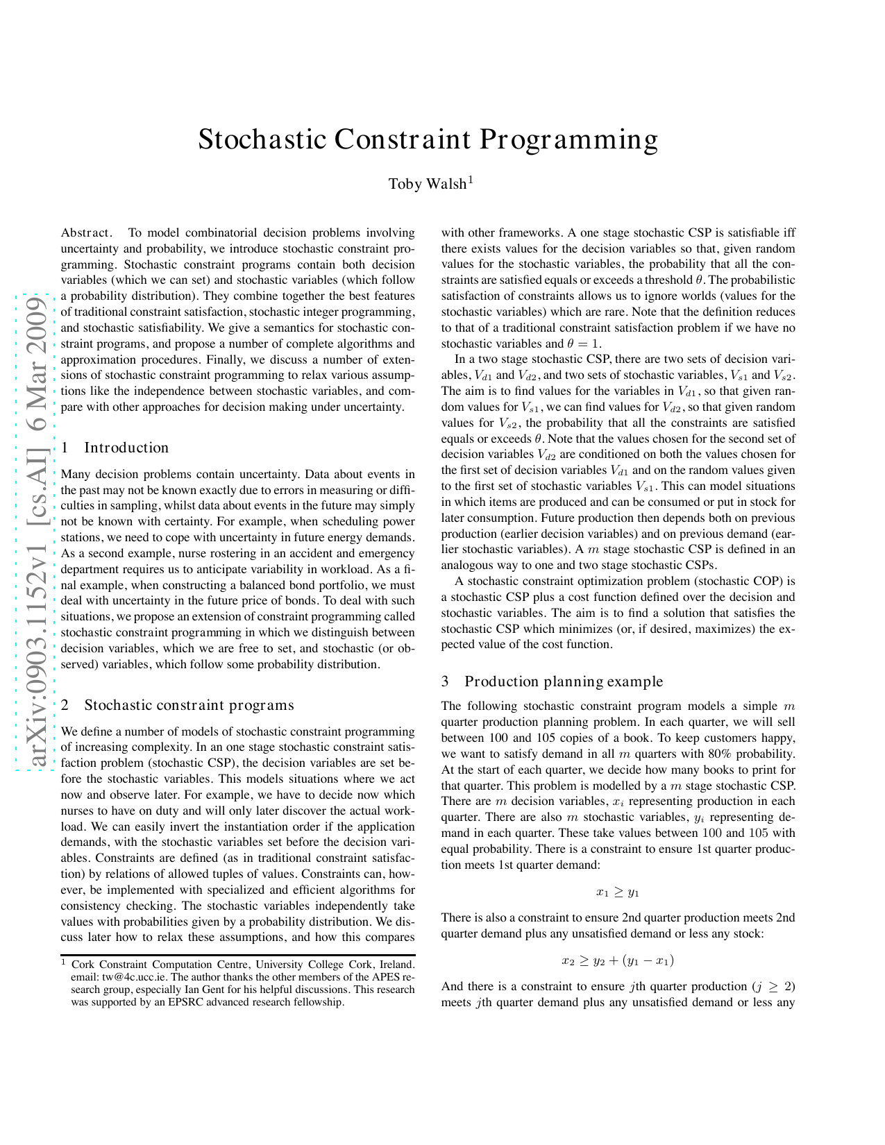
The following stochastic constraint program models a simple m quarter production planning problem. In each quarter, we will sell between 100 and 105 copies of a book. To keep customers happy, we want to satisfy demand in all m quarters with 80% probability. At the start of each quarter, we decide how many books to print for that quarter. This problem is modelled by a m stage stochastic CSP. There are m decision variables, xi representing production in each quarter. There are also m stochastic variables, yi representing demand in each quarter. These take values between 100 and 105 with equal probability. There is a constraint to ensure 1st quarter production meets 1st quarter demand:
There is also a constraint to ensure 2nd quarter production meets 2nd quarter demand plus any unsatisfied demand or less any stock:
And there is a constraint to ensure jth quarter production (j ≥ 2) meets jth quarter demand plus any unsatisfied demand or less any stock:
We must satisfy these m constraints with a threshold probability θ = 0.8. This stochastic CSP has a number of solutions including xi = 105 for each i (i.e. always produce as many books as the maximum demand). However, this solution will tend to produce books surplus to demand which is undesirable.
Suppose storing surplus book costs $1 per quarter. We can define a m stage stochastic COP based on this stochastic CSP in w
…(Full text truncated)…
This content is AI-processed based on ArXiv data.