Polar Codes are Optimal for Lossy Source Coding

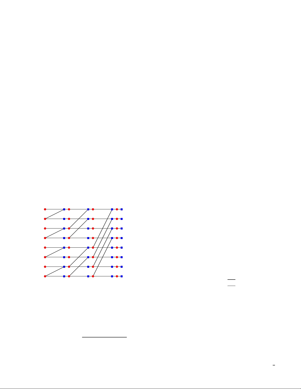
1 Polar Codes are Optimal for Lo ssy Source Coding Satish Babu K orada and R ¨ udiger Urban ke Abstract — W e consider lossy source compression of a bi nary symmetric source using polar codes and the low-complexity successiv e enco ding algorithm. It was recently sh own by Arık an that polar codes achiev e the capacity of arbitrary symmetric binary-input discre te memory less chann els under a successive decoding strategy . W e show the equivalent r esult for lossy source compression, i.e., we sh ow that this combination achiev es the rate-distortion bound for a binary symmetric source. W e further show the optimality of polar codes for va rious pr oblems including the binary Wy ner -Ziv and the binary Gelfand-Pinsker problem. I . I N T RO D U C T I O N Lossy so urce compr ession is o ne of the f undame ntal pro b- lems of infor mation theo ry . Consider a binary symmetr ic source (BSS) Y . Let d ( · , · ) d enote the Hammin g distortion function , d (0 , 0 ) = d (1 , 1) = 0 , d (0 , 1) = 1 . It is well known that in ord er to compress Y with a verage distortion D the rate R has to be at least R ( D ) = 1 − h 2 ( D ) , where h 2 ( · ) is the b inary entro py functio n [1], [2 , Theor em 10.3.1 ]. Sh annon ’ s p roof of this rate-distor tion boun d is based on a rando m coding argum ent. It was shown by Goblick that in fact linear codes are sufﬁcient to achieve th e rate-distor tion b ound [3],[4 , Section 6.2.3] . T rellis based quantizers [5] were perhaps t he ﬁrst “practical” solution to so urce co mpression. Their enc oding complexity is linear in the blo cklength of th e code (V iter bi alg orithm). For any rate strictly larger than R ( D ) the gap between the expected distortion and the design distortion D vanishes exponentially in the constraint length . Howe ver , the com plexity of the en- coding algor ithm also scales expo nentially with the c onstraint length. Giv en the s uccess of sparse graph codes combined with lo w- complexity message-passing algorithms for the channel coding problem , it is interesting to in vestigate the per forman ce of such a co mbination for lossy sour ce c ompression . As a ﬁrst question, we can ask if the codes themselves are suitable for the task. I n this respect, Matsun aga and Y amamoto [6] showed that if the degrees of a low-density p arity-check (LDPC) en semble are chosen as large as Θ(lo g( N )) , where N is the blocklen gth, th en this ensemble saturates the rate- distortion bo und if optimal e ncoding is employed. Even m ore promising , M artininian and W ainwright [7] proved that p rop- erly chosen MN codes with bou nded degree s are sufﬁcient to achieve the rate-distortion boun d under op timal enco ding. EPFL, School of Computer , & Communication Scienc es, L ausanne, CH- 1015, Switzerland, { satish.kora da, ruediger . urbank e } @epﬂ.ch. This wor k was partia lly supporte d by the Natio nal Compete nce Center in Research on Mobile Information and Communicat ion Systems (NCCR-MICS), a center supported by the Swiss National Scienc e Foundati on under grant number 5005-67322. Much less is known abo ut the perfo rmance o f sparse graph codes under message-passing encod ing. In [8] the authors consider binary er asure qu antization, th e so urce-co mpression equiv alent of the binar y e rasure channel (BEC) co ding prob- lem. They show that LDPC-based q uantizers fail if the parity check density is o (log( N )) but tha t prop erly co nstructed low- density g enerator-matrix (LDGM) based qu antizers comb ined with message-passing enco ders a re optimal. They exploit the close relationsh ip between the channel coding prob lem and the lossy so urce co mpression p roblem, togethe r with the fact that LDPC codes achieve the cap acity of the BEC un der message- passing dec oding, to prove the latter claim. Regular LDGM codes were considered in [9]. Using non- rigoro us methods fr om statistical physics it was shown tha t these codes appr oach r ate-distortion bound for large degrees. It was empir ically shown that these code s have good per- forman ce under a variant o f belief propag ation algorithm (reinfo rced belief propagatio n). In [10] the authors con sider check-r egular LDGM code s an d show using non -rigor ous methods th at these codes appr oach the rate-distortion b ound for large check degree. Moreover, for a ny rate strictly larger than R ( D ) , the gap betwee n the achieved distortion and D vanishes exponentially in the ch eck degree. They also observe that belief pro pagation inspired decim ation (BID) algorithm s do not p erform well in this context. In [11], survey propag ation inspired dec imation (SID) was proposed as an iterativ e algorithm for ﬁnding the solution s of K-SA T (n on- linear co nstraints) f ormulae efﬁciently . Based on this success, the authors in [10] r eplaced the p arity-ch eck nodes with n on- linear co nstraints, and empirically showed that using SID one can achieve a perfor mance close to the r ate-distortion boun d. The co nstruction in [8] sug gests that those LDGM codes whose duals (LDPC) are o ptimized for the binary symmet- ric chan nel (BSC) m ight be good can didates for the lossy compression of a BSS using message-passing enco ding. I n [12] th e authors consider such LDGM cod es and e mpirically show that by using SID one ca n appr oach very close to the rate-distortio n b ound. They also mention that even BID works well but that it is not as go od as SID. Recently , in [1 3] it was experimentally sho wn that using BID it is po ssible to approach the rate-distortio n bou nd clo sely . The key to m aking b asic BP work well in this c ontext is to cho ose the cod e pro perly . Th is suggests that in fact th e more sop histicated algo rithms like SID ma y not e ven be necessary . In [14] the authors consider a dif feren t approach. They show that f or any ﬁxed γ , ǫ > 0 the rate-distor tion pair ( R ( D ) + γ , D + ǫ ) can be achieved with co mplexity C 1 ( γ ) ǫ − C 2 ( γ ) N . Of course, the complexity diverges as γ and ǫ are made smaller . The idea there is to concatenate a small code of rate R + γ with expected distortion D + ǫ . The source seq uence is then split into blocks of size equal to the code. The concentratio n with 2 respect to the blocklen gth implies th at u nder MAP deco ding the p robability that the distortion is larger than D + ǫ vanishes. Polar co des, introd uced b y Ar ıkan in [15], are the ﬁrst provably capacity achieving codes fo r arbitrary symmetric binary- input discrete memor yless chann els (B-DMC) with low encodin g and d ecoding c omplexity . These cod es are naturally suited f or deco ding via successiv e cancellation (SC) [15 ]. It was pointed out i n [15] that an SC decod er can be impleme nted with Θ ( N lo g( N )) comp lexity . W e show that polar cod es with an SC encoder are also optimal for lossy sourc e c ompression . More precisely , we show that fo r any de sign d istortion 0 < D < 1 2 , and any δ > 0 an d 0 < β < 1 2 , the re exists a sequen ce of polar cod es of rate at most R ( D ) + δ and increasing len gth N so that their expected distortion is at mo st D + O (2 − ( N β ) ) . Th eir enco ding as well as deco ding com plexity is Θ( N log( N )) . I I . I N T RO D U C T I O N T O P O L A R C O D E S Let W : { 0 , 1 } → Y be a binary-input discre te me m- oryless chan nel (B-DMC). Let I ( W ) ∈ [0 , 1 ] denote the mutual info rmation between the input and o utput of W with unifor m distribution o n the inputs, call it the sy mmetric mutual informatio n. Clearly , if the chann el W is symmetr ic, then I ( W ) is the capacity o f W . Also, let Z ( W ) ∈ [0 , 1] denote the Bhattach aryya parameter of W , i.e., Z ( W ) = P y ∈Y p W ( y | 0 ) W ( y | 1 ) . In the following, an upper case letter U deno tes a r andom variable and and u d enotes its r ealization. Let ¯ U denote the random vector ( U 0 , . . . , U N − 1 ) . For any set F , | F | deno tes its car dinality . Let ¯ U F denote ( U i 1 , . . . , U i | F | ) an d let ¯ u F denote ( u i 1 , . . . , u i | F | ) , where { i k ∈ F : i k ≤ i k +1 } . Let U j i denote the r andom vector ( U i , . . . , U j ) an d, similarly , u j i denotes ( u i , . . . , u j ) . W e use the equivalent n otation for o ther random variables like X or Y . Let Ber ( p ) denote a Ber noulli random variable with Pr(1) = p . The p olar code constructio n is based o n th e following observation. Let G 2 =  1 0 1 1  . (1) Let A n : { 0 , . . . , 2 n − 1 } → { 0 , . . . , 2 n − 1 } be a permutatio n deﬁned b y the bit-reversal ope ration in [15]. Apply the transfo rm A n G ⊗ n 2 (where “ ⊗ n ” den otes the n th Kronecker power) to a bloc k of N = 2 n bits and transmit the outp ut thro ugh indepen dent copies o f a B-DMC W (see Figure 1). As n g rows large, the channe ls seen by individual bits ( suitably deﬁned in [15 ]) start po larizing : they app roach either a noiseless ch annel or a pu re-noise channel, wh ere the fr action of channels becomin g noiseless is close to the symmetric m utual inform ation I ( W ) . In wh at follows, let H n = A n G ⊗ n 2 . Consider a r andom vector ¯ U that is u niform ly d istributed over { 0 , 1 } N . Let ¯ X = ¯ U H n , where the m ultiplication is perfor med over GF(2). L et ¯ Y be the result of sen ding the co mpon ents o f ¯ X over the channel W . Let P ( ¯ U , ¯ X , ¯ Y ) denote the ind uced prob ability distribution o n the set { 0 , 1 } N × { 0 , 1 } N × Y N . The ch annel W · · · W A n G ⊗ n U 0 U 1 · · · U N − 1 X 0 X N − 1 Y 0 · · · Y N − 1 Fig. 1. The transform A n G ⊗ n 2 is applied to the informati on word ¯ U and the resulting vect or ¯ X is transmitte d through the channel W . The recei ved word is ¯ Y . between ¯ U and ¯ Y is d eﬁned b y the tra nsition pr obabilities P ¯ Y | ¯ U ( ¯ y | ¯ u ) = N − 1 Y i =0 W ( y i | x i ) = N − 1 Y i =0 W ( y i | ( ¯ uH n ) i ) . Deﬁne W ( i ) : { 0 , 1 } → Y N × { 0 , 1 } i − 1 as the channel with input u i , output ( y N − 1 0 , u i − 1 0 ) , and transition probabilities giv en by W ( i ) ( ¯ y , u i − 1 0 | u i ) , P ( ¯ y , u i − 1 0 | u i ) = X u N − 1 i +1 P ( ¯ y | ¯ u ) P ( ¯ u ) P ( u i ) = 1 2 N − 1 X u N − 1 i +1 P ¯ Y | ¯ U ( ¯ y | ¯ u ) . (2) Let Z ( i ) denote th e Bhattach aryya para meter of the ch annel W ( i ) , Z ( i ) = X y N − 1 0 ,u i − 1 0 q W ( i ) ( y N − 1 0 , u i − 1 0 | 0) W ( i ) ( y N − 1 0 , u i − 1 0 | 1) . (3) The SC d ecoder operates as f ollows: the bits U i are deco ded in the ord er 0 to N − 1 . The likelihood of U i is comp uted using the chan nel law W ( i ) ( ¯ y , ˆ u i − 1 0 | u i ) , where ˆ u i − 1 0 are the estimates of the b its U i − 1 0 from the previous decoding steps. In [15] it was sho wn that the f raction of the channels W ( i ) that are appro ximately noiseless approaches I ( W ) . Mo re precisely , it was shown th at the { Z ( i ) } satisfy lim n →∞ | n i ∈ { 0 , . . . , 2 n − 1 } : Z ( i ) < 2 − 5 n 4 o | 2 n = I ( W ) . (4) In [16 ], the above result was signiﬁcantly stren gthened to lim n →∞ | n i ∈ { 0 , . . . , 2 n − 1 } : Z ( i ) < 2 − 2 nβ o | 2 n = I ( W ) , ( 5) which is valid fo r any 0 ≤ β < 1 2 . This sug gests to use these noiseless channels (i.e ., tho se channels at position i so tha t Z ( i ) < 2 − 2 nβ ) for transmitting informa tion while ﬁx ing the symbols transmitted th rough th e remaining channels to a value known both to sender as we ll to th e receiver . Following Arıkan, call those compo nents U i of ¯ U which are ﬁxed “frozen, ” (den ote th is set of positions as F ) and the r emaining on es “inf ormation ” b its. If th e ch annel 3 W is symmetr ic we can assum e without loss of gener ality that the ﬁxed po sitions are set to 0 . In [ 15] it was shown that the block error p robability o f the SC decod er is bo unded by P i ∈ F Z ( i ) , which is of ord er O (2 − 2 nβ ) fo r our c hoice. Since the fr action o f appr oximately n oiseless channels tends to I ( W ) , this schem e ac hieves the capa city of the un derlying symmetric B-DM C W . In [15] the f ollowing alternative interpretation was men- tioned; th e a bove proced ure can be seen as transmitting a codeword of a code deﬁned thr ough its ge nerator matrix as follows. A p olar co de of dimension 0 ≤ k ≤ 2 n is deﬁned by choosing a subset of the rows of H n as the generator matrix. The cho ice of the g enerator vectors is based on the values of Z ( i ) . A polar code is th en deﬁned as the set of codew ords of the form ¯ x = ¯ uH n , where the bits i ∈ F are ﬁxed to 0 . The well k nown Reed-Muller c odes can be con sidered as special cases of polar codes with a particular ru le f or the ch oice of F . Polar c odes with SC d ecoding have an in teresting, an d o f as yet not fully exp lored, co nnection to the recursive decoding of Reed-Muller codes as prop osed b y Dumer [ 17]. The Plotkin ( u, u + v ) co nstruction in Dum er’ s algor ithm plays the role of th e cha nnel comb ining and chann el splitting for polar codes. Perh aps the two most im portant differences are ( i) th e construction of the code itself (h ow the fro zen vector s are chosen), and (ii) th e actua l deco ding algo rithm and the orde r in wh ich info rmation bits are deco ded. A better understand ing of this conne ction might lead to improved d ecoding algorithms for bo th con structions. X 7 X 6 X 5 X 4 X 3 X 2 X 1 X 0 U 7 U 3 U 5 U 1 U 6 U 2 U 4 U 0 W ( y 7 | x 7 ) . . . . . . . . . W ( y 0 | x 0 ) Fig. 2. Fact or graph representa tion used by the S C decoder . W ( y i | x i ) is the initia l prior of the v ariable X i , when y i is recei ved at the output of a symmetric B-DMC W . T o summ arize, the SC decod er operates as follows. For each i in the rang e 0 till N − 1 : (i) If i ∈ F , then set u i = 0 . (ii) If i ∈ F c , the n comp ute l i ( ¯ y , u i − 1 0 ) = W ( i ) ( ¯ y , u i − 1 0 | u i = 0) W ( i ) ( ¯ y , u i − 1 0 | u i = 1) and set u i =  0 , if l i > 1 , 1 , if l i ≤ 1 . (6) As explain ed in [15] using th e factor grap h rep resentation shown in Figu re 2, the SC deco der can be implemen ted with complexity Θ( N lo g( N )) . A similar rep resentation was considered for deco ding of Reed-Mu ller codes by Forney in [18]. A. Decimatio n and R andom Rou nding In the setting of ch annel codin g there is typ ically one codeword (namely the tran smitted one) which ha s a po sterior that is signiﬁcan tly larger than all other codewords. This makes it possible for a gr eedy message- passing algorith m to successfully move towards this codew ord in small steps, using at any given moment “local” inf ormation provid ed by the decoder . In the case of lossy sou rce comp ression there ar e typically many co dew ord s that, if ch osen, result in similar distortion. Let us assume that these “cand idates” are ro ughly unif ormly spread aroun d the source word to be compressed. It is then clear th at a local decoder c an easily g et “conf used, ” prod ucing locally co nﬂicting in formatio n with regards to the “dire ction” into which one sho uld compr ess. A standard way to overcome this problem is to comb ine the message-passing algor ithm with decimation steps. This work s as fo llows; ﬁrst run th e iterative algorithm for a ﬁxed nu mber of iteratio ns and subsequently decimate a small fr action of th e bits. Mor e precisely , this means that for each bit which we decide to decima te we choose a value . W e the n remove the decimated variable no des and adjacent edg es from the grap h. One is hence left with a smaller instance of essentially th e same pr oblem. The same pro cedure is then re peated on the reduced gr aph an d this cycle is continu ed until a ll variables have been d ecimated. One can interpr et the SC operation as a kind o f decim a- tion where the order of the dec imation is ﬁxed in advance ( 0 , . . . , N − 1 ). In fact, the SC d ecoder can b e in terpreted as a pa rticular instance o f a BID. When mak ing the decision on bit U i using th e SC d ecoder, it is natural to choo se th at value fo r U i which m aximizes the posterior . I ndeed, such a sche me works well in p ractice for source compression. For th e analysis however it is mo re conv enient to u se randomized r ound ing . I n ea ch step, instead of mak ing the MAP decision we replace (6) with u i =  0 , w .p. l i 1+ l i , 1 , w .p. 1 1+ l i . In words, we make the decision pro portiona l to the likelihoods. Randomized roun ding as a decimatio n rule is not new . E.g., in [19] it was used to analyze the performa nce of BID for random K -SA T problem s. For lossy source compression , the SC op eration is employed at th e e ncoder side to map the source vector to a codeword. Therefo re, fro m n ow onwards we refer to this op eration as SC encodin g . I I I . M A I N R E S U LT A. Sta tement Theor em 1 ( P olar Cod es Achieve the Rate- Distortion Bound ): Let Y b e a BSS and ﬁx the d esign distortion D , 0 < D < 1 2 . 4 For any rate R > 1 − h 2 ( D ) and any 0 < β < 1 2 , there exists a sequ ence of polar codes of leng th N with rates R N < R so that un der SC encodin g using rand omized r oundin g they achieve expected distortion D N satisfying D N ≤ D + O (2 − ( N β ) ) . The encoding as well as decodin g complexity o f th ese codes is Θ( N log( N )) . B. Simu lation Results and Discussion Let us consider how po lar cod es be have in practice. Recall that the length N of the code is always a power of 2 , i.e. , N = 2 n . L et us construct a p olar co de to achieve a distor tion D . Let W deno te the channel BSC ( D ) an d let R = R ( D ) + δ for som e δ > 0 . In order to fully specify the code we nee d to specify the set F , i.e. , th e set of f rozen compo nents. W e pro ceed as follows. First we estimate the Z ( i ) s fo r all i ∈ { 0 , N − 1 } and so rt the indices i in decre asing order of Z ( i ) s. The set F co nsists of the ﬁrst R N ind ices, i.e., it co nsists of the indices correspon ding to th e RN largest Z ( i ) s. This is similar to the chann el cod e co nstruction fo r the BSC ( D ) but ther e is a slight dif feren ce. For the case of channel coding we assign all in dices i so that Z ( i ) is v ery small, i.e., so that lets say Z ( i ) < δ , to the set F c . Therefo re, the set F consists of all tho se ind ices i so that Z ( i ) ≥ δ . For the sou rce co mpression, o n th e other hand, F con sists of all those indice s i so that Z ( i ) ≥ 1 − δ , i.e., of all those indices cor respond ing to very large values of Z ( i ) . Putting it differently , in chan nel co ding, th e rate R is chosen to be strictly less th an 1 − h 2 ( D ) , wher eas in source compression it is cho sen so that it is strictly larger th an this quantity . Figure 3 shows the p erform ance of the SC encodin g algorithm c ombined with rand omized roun ding. A s asserted by Th eorem 1 , th e p oints ap proach th e r ate-distortion bound as the block leng th incre ases. 0 . 0 0 . 2 0 . 4 0 . 6 0 . 8 0 . 1 0 . 2 0 . 3 0 . 4 D R Fig. 3. The rate-distor tion performance for the SC encod ing algorithm with randomize d rounding for n = 9 , 11 , 13 , 15 , 17 and 19 . As the block length increa ses the points mov e closer to the rate-distor tion bound. In [20] the p erform ance of polar codes fo r lossy source compression was alread y inv estigated emp irically . Note that the constru ction used in [20] is different f rom th e curren t construction . Let us recall. Consider a BSC ( p ) , where p = h − 1 2 (1 − h 2 ( D )) . Let the correspon ding Bha ttacharyya con- stants be ˜ Z ( i ) s. In [2 0] ﬁrst a chann el code of rate 1 − h 2 ( p ) − ǫ is co nstructed acc ording to the values ˜ Z ( i ) s. Let ˜ F be the correspo nding froze n set. The set F for the source cod e is giv en by F = { N − 1 − i : i ∈ ˜ F c } . The rationale b ehind this construction is that the resulting source cod e is the du al of the channel c ode design ed for the BSC ( p ) . The rate of th e resulting source code is equ al to h 2 ( p ) + ǫ = 1 − h 2 ( D ) + ǫ . Although this co de construction is different, empirica lly the resu lting f rozen sets are very similar . There is also a slight difference with resp ect to the decima- tion algorithm. In [ 20] th e decimation step is b ased o n MAP estimates, whereas in the curr ent setting we use random ized round ing. Despite all th ese d ifferences the perform ance of both schemes is compa rable. I V . T H E P RO O F From now on we restrict W to b e a BSC ( D ) , i.e. , W (0 | 1) = W (1 | 0) = D , W (0 | 0) = W (1 | 1) = 1 − D . As immed iate conseq uence we have W ( y | x ) = W ( y ⊕ z | x ⊕ z ) . (7) This extends in a natu ral way if we co nsider vectors. A. The S tanda r d S our ce Coding Model Let us describe lo ssy source compression using polar codes in more detail. W e refer to this as the “Standard Model. ” In the f ollowing we assume that we want to comp ress the source with average distortion D . Model: Let ¯ y = ( y 0 , . . . , y N − 1 ) denote N i.i.d. realizatio ns of the sou rce Y . Let F ⊆ { 0 , . . . , N − 1 } an d let ˜ u F ∈ { 0 , 1 } | F | be a ﬁxed vector . In the sequel we use the shorth and “SM ( F, ˜ u F ) ” to de note the Stand ard Mode l with frozen set F whose com ponen ts are ﬁxed to ˜ u F . It is d eﬁned as follows. Encodin g: Let f ˜ u F : { 0 , 1 } N → { 0 , 1 } N −| F | denote th e encodin g fu nction. F or a giv en ¯ y we ﬁrst compute ¯ u , as described below , wh ere ¯ u = ( u 0 , . . . , u N − 1 ) . Then f ˜ u F ( ¯ y ) = ¯ u F c . Giv en ¯ y , for each i in the r ange 0 till N − 1 : (i) Compute l i ( ¯ y , u i − 1 0 ) , W ( i ) ( ¯ y , u i − 1 0 | u i = 0) W ( i ) ( ¯ y , u i − 1 0 | u i = 1) . (ii) If i ∈ F c then set u i = 0 with pro bability l i 1+ l i and eq ual to 1 otherwise; if i ∈ F th en set u i = ˜ u i . Decoding : The decoding fu nction ˆ f ˜ u F : { 0 , 1 } N −| F | → { 0 , 1 } N maps ¯ u F c back to the r econstruction point ¯ x via ¯ x = ¯ uH n , where ¯ u F = ˜ u F . Distortion: The average d istortion incurre d b y this scheme is given b y E [ d ( ¯ Y , ¯ X )] , where th e expectation is over the 5 source ra ndomn ess and the rand omness in volved in the ran- domized ro unding at the encod er . Complexity: The encodin g (decod ing) task for source codin g is the same as the decodin g (encod ing) task for channel co ding. As rema rked before, bo th have comp lexity Θ ( N lo g N ) . Remark: Recall that l i is the posterio r of the variable U i giv en the observations ¯ Y as well as ¯ U i − 1 0 , under the assumption that ¯ U has un iform prio r a nd that ¯ Y is the re sult of tran smitting ¯ U H n over a BSC ( D ) . B. Compu tation of A verag e Distortion The enco ding function f ˜ u F is rand om. More prec isely , in step i of the encoding p rocess, i ∈ F c , we ﬁx the value of U i propo rtional to the posterior (rand omized ro unding ) P U i | U i − 1 0 , ¯ Y ( u i | u i − 1 0 , ¯ y ) . This imp lies th at th e pro bability of picking a vector ¯ u given ¯ y is equal to ( 0 , ¯ u F 6 = ˜ u F , Q i ∈ F c P U i | U i − 1 0 , ¯ Y ( u i | u i − 1 0 , ¯ y ) , ¯ u F = ˜ u F . Therefo re, the average (over ¯ y and the rand omness of the encoder ) distortio n of SM ( F, ˜ u F ) is giv en by D N ( F, ˜ u F ) = X ¯ y ∈{ 0 , 1 } N 1 2 N X ¯ u F c ∈{ 0 , 1 } | F c | Y i ∈ F c P ( u i | u i − 1 0 , ¯ y ) d ( ¯ y , ¯ uH n ) , (8) where U i = ˜ u i for i ∈ F . W e want to to show that there exists a set F of card inality rough ly N h 2 ( D ) an d a vecto r ˜ u F such th at D N ( F, ˜ u F ) ≈ D . T his will show that polar codes ac hieve the rate-distor tion bound . For the pro of it is m ore co n venient no t to deter mine th e distortion for a ﬁxed choice of ˜ u F but to co mpute the average distortion over all possible choices (with a uniform distrib ution over these choices). Later, in Section V, we will see that the distortion do es not depend on the choice o f ˜ u F . A co n venient choice is therefore to set it to zero. This will lead to the desired ﬁnal r esult. Let us therefore start by com puting the aver age distor- tion . Let D N ( F ) denote the d istortion o btained by averaging D N ( F, ˜ u F ) over all 2 | F | possible values o f ˜ u F . W e will show that D N ( F ) is close to D . The distor tion D N ( F ) can be written as D N ( F ) = X ˜ u F ∈{ 0 , 1 } | F | 1 2 | F | D N ( F, ˜ u F ) = X ˜ u F 1 2 | F | X ¯ y 1 2 N X ¯ u F c Y i ∈ F c P ( u i | u i − 1 0 , ¯ y ) d ( ¯ y , ¯ uH n ) = X ¯ y 1 2 N X ¯ u 1 2 | F | Y i ∈ F c P ( u i | u i − 1 0 , ¯ y ) d ( ¯ y , ¯ uH n ) . Let Q ¯ U , ¯ Y denote th e distribution d eﬁned by Q ¯ Y ( ¯ y ) = 1 2 N and Q ¯ U | ¯ Y deﬁned by Q ( u i | u i − 1 0 , ¯ y ) =  1 2 , if i ∈ F, P U i | U i − 1 0 , ¯ Y ( u i | u i − 1 0 , ¯ y ) , if i ∈ F c . (9) Then, D N ( F ) = E Q [ d ( ¯ Y , ¯ U H n )] , where E Q [ · ] deno tes expectatio n with respect to th e distribu- tion Q ¯ U , ¯ Y . Similarly , let E P [ · ] denote the expectation with respect to the distribution P ¯ U , ¯ Y . Recall that P ¯ Y ( ¯ y ) = 1 2 N and that we can write P ¯ U | ¯ Y in th e fo rm P ¯ U | ¯ Y ( ¯ u | ¯ y ) = N − 1 Y i =0 P U i | U i − 1 0 , ¯ Y ( u i | u i − 1 0 , ¯ y ) . If we compar e Q to P we see that they hav e the same structure except for the c ompon ents i ∈ F . Ind eed, in the f ollowing lemma we show that th e total variation distance between Q and P can be boun ded in ter ms o f how much the posterio rs Q U i | U i − 1 0 , ¯ Y and P U i | U i − 1 0 , ¯ Y differ fo r i ∈ F . Lemma 2 (Boun d on the T otal V ariation Distance ): Let F denote the set o f fr ozen indic es and let the probability dis- tributions Q and P be as deﬁned ab ove. Then X ¯ u, ¯ y | Q ( ¯ u , ¯ y ) − P ( ¯ u, ¯ y ) | ≤ 2 X i ∈ F E P     1 2 − P U i | U i − 1 0 , ¯ Y (0 | U i − 1 0 , ¯ Y )     . Pr oof: X ¯ u | Q ( ¯ u | ¯ y ) − P ( ¯ u | ¯ y ) | = X ¯ u    N − 1 Y i =0 Q ( u i | u i − 1 0 , ¯ y ) − N − 1 Y i =0 P ( u i | u i − 1 0 , ¯ y )    = X ¯ u    N − 1 X i =0 h  Q ( u i | u i − 1 0 , ¯ y ) − P ( u i | u i − 1 0 , ¯ y )  ·  i − 1 Y j =0 P ( u j | u j − 1 0 , ¯ y )  N − 1 Y j = i +1 Q ( u j | u j − 1 0 , ¯ y ) i    . In the last step we have used the f ollowing telescoping expansion: A N − 1 0 − B N − 1 0 = N − 1 X i =0 A i 0 B N − 1 i +1 − N − 1 X i =0 A i − 1 0 B N − 1 i , where A j k denotes h ere the p roduc t Q j i = k A i . Now note th at if i ∈ F c then Q ( u i | u i − 1 0 , ¯ y ) = P ( u i | u i − 1 0 , ¯ y ) , so that these terms vanish. Th e above su m therefor e redu ces to X ¯ u    X i ∈ F h  Q ( u i | u i − 1 0 , ¯ y ) − P ( u i | u i − 1 0 , ¯ y )  | {z } ≤ | 1 2 − P ( u i | u i − 1 0 , ¯ y ) | · 6  i − 1 Y j =0 P ( u j | u j − 1 0 , ¯ y )  N − 1 Y j = i +1 Q ( u j | u j − 1 0 , ¯ y ) i    ≤ X i ∈ F X ¯ u i 0    1 2 − P ( u i | u i − 1 0 , ¯ y )    i − 1 Y j =0 P ( u j | u j − 1 0 , ¯ y ) ≤ 2 X i ∈ F E P ¯ U | ¯ Y = ¯ y     1 2 − P U i | U i − 1 0 , ¯ Y (0 | U i − 1 0 , ¯ y )     . In the last step the summation over u i giv es rise to the factor 2 , whereas the summation over u i − 1 0 giv es rise to the e xpecta tion. Note tha t Q ¯ Y ( ¯ y ) = P ¯ Y ( ¯ y ) = 1 2 N . The claim follows b y taking th e expectation over ¯ Y . Lemma 3 (Distortion u nder Q versus Distortion un der P ): Let F b e chosen such that for i ∈ F E P     1 2 − P U i | U i − 1 0 , ¯ Y (0 | U i − 1 0 , ¯ Y )     ≤ δ N . (10) The average d istortion is then bo unded by 1 N E Q [ d ( ¯ Y , ¯ U H n )] ≤ 1 N E P [ d ( ¯ Y , ¯ U H n )] + | F | 2 δ N . Pr oof: E Q [ d ( ¯ Y , ¯ U H n )] − E P [ d ( ¯ Y , ¯ U H n )] = X ¯ u, ¯ y  Q ( ¯ u , ¯ y ) − P ( ¯ u, ¯ y )  d ( ¯ y , ¯ uH n ) ≤ N X ¯ u, ¯ y    Q ( ¯ u , ¯ y ) − P ( ¯ u, ¯ y )    Lem. 2 ≤ 2 N X i ∈ F E P     1 2 − P U i | U i − 1 0 , ¯ Y (0 | U i − 1 0 , ¯ Y )     ≤ | F | 2 N δ N . From Lem ma 3 we see tha t the a verage ( over ¯ y a s w ell as ˜ u F ) d istortion o f th e Stand ard Mode l is uppe r bou nded b y the av erage distor tion with respect to P plu s a ter m which b ounds the “d istance” between Q and P . Lemma 4 (Distortion u nder P ): E P [ d ( ¯ Y , ¯ U H n )] = N D . Pr oof: Let ¯ X = ¯ U H n and write E P [ d ( ¯ Y , ¯ U H n )] = X ¯ u, ¯ y P ¯ U , ¯ Y ( ¯ u , ¯ y ) d ( ¯ y, ¯ u H n ) = X ¯ y , ¯ u, ¯ x P ¯ U , ¯ X , ¯ Y ( ¯ u , ¯ x, ¯ y ) d ( ¯ y, ¯ uH n ) = X ¯ y , ¯ u, ¯ x P ¯ X , ¯ Y ( ¯ x, ¯ y ) P ¯ U | ¯ X , ¯ Y ( ¯ u | ¯ x, ¯ y ) | {z } { 0 , 1 } -valued d ( ¯ y , ¯ x ) = X ¯ y, ¯ x P ¯ X , ¯ Y ( ¯ x , ¯ y ) d ( ¯ y , ¯ x ) . Note that the un condition al distribution of ¯ X as well as ¯ Y is the un iform o ne and that the chann el between ¯ X and ¯ Y is memory less and identical for each comp onent. Theref ore, we can write this expec tation as E P [ d ( ¯ Y , ¯ U H n )] = N X x 0 ,y 0 P X 0 ,Y 0 ( x 0 , y 0 ) d ( y 0 , x 0 ) ( a ) = N X x 0 P X 0 ( x 0 ) X y 0 W ( y 0 | x 0 ) d ( y 0 , x 0 ) = N W (0 | 1) ( b ) = N D . In the above equation, ( a ) follows fr om the fact that P Y | X ( y | x ) = W ( y | x ) , and ( b ) fo llows from our assumption that W is a BSC ( D ) . This implies that if we use all the variables { U i } to represent the so urce word, i.e., F is e mpty , then the algorithm results in an a verage distortion D . But the rate of such a code would b e 1 . Fortun ately , the last prob lem is e asily ﬁxed. I f we ch oose F to consist of those variables which a re “essentially rand om, ” then there is o nly a small distor tion penalty (nam ely , | F | 2 δ N ) to p ay with respe ct to the previous case. But the rate has be en decreased to 1 − | F | / N . Lemma 3 shows that the g uiding princip le for choo sing the set F is to include the indices with small δ N in (10). In the following lemm a, we ﬁnd a sufﬁcient con dition for an index to satisfy (10), which is e asier to handle. Lemma 5 ( Z ( i ) Close to 1 is Good ): I f Z ( i ) ≥ 1 − 2 δ 2 N , then E P     1 2 − P U i | U i − 1 0 , ¯ Y (0 | U i − 1 0 , ¯ Y )     ≤ δ N . Pr oof: E P h q P U i | U i − 1 0 , ¯ Y (0 | U i − 1 0 , ¯ Y ) P U i | U i − 1 0 , ¯ Y (1 | U i − 1 0 , ¯ Y ) i = X u i − 1 0 , ¯ y P U i − 1 0 , ¯ Y ( u i − 1 0 , ¯ y ) q P U i | U i − 1 0 , ¯ Y (0 | u i − 1 0 , ¯ y ) P U i | U i − 1 0 , ¯ Y (1 | u i − 1 0 , ¯ y ) = X u i − 1 0 , ¯ y q P U i − 1 0 ,U i , ¯ Y ( u i − 1 0 , 0 , ¯ y ) P U i − 1 0 ,U i , ¯ Y ( u i − 1 0 , 1 , ¯ y ) = X u i − 1 0 , ¯ y v u u t X u N − 1 i +1 P ¯ U , ¯ Y (( u i − 1 0 , 0 , u N − 1 i +1 ) , ¯ y ) v u u t X u N − 1 i +1 P ¯ U , ¯ Y (( u i − 1 0 , 1 , u N − 1 i +1 ) , ¯ y ) ( a ) = 1 2 N X u i − 1 0 , ¯ y v u u t X u N − 1 i +1 P ¯ Y | ¯ U ( ¯ y | u i − 1 0 , 0 , u N − 1 i +1 ) v u u t X u N − 1 i +1 P ¯ Y | ¯ U ( ¯ y | u i − 1 0 , 1 , u N − 1 i +1 ) = 1 2 Z ( i ) . The eq uality ( a ) follows fro m the fact that P ¯ U ( ¯ u ) = 1 2 N for all ¯ u ∈ { 0 , 1 } N . Assume now that Z ( i ) ≥ 1 − 2 δ 2 N . Th en E P  1 2 − q P U i | U i − 1 0 , ¯ Y (0 | U i − 1 0 , ¯ Y ) P U i | U i − 1 0 , ¯ Y (1 | U i − 1 0 , ¯ Y )  ≤ δ 2 N . Multiplying an d dividing the term inside the expectation with 1 2 + q P U i | U i − 1 0 , ¯ Y (0 | u i − 1 0 , ¯ y ) P U i | U i − 1 0 , ¯ Y (1 | u i − 1 0 , ¯ y ) , 7 and upper bou nding this ter m in the denomin ator with 1 , we get E P  1 4 − P U i | U i − 1 0 , ¯ Y (0 | U i − 1 0 , ¯ Y ) P U i | U i − 1 0 , ¯ Y (1 | U i − 1 0 , ¯ Y )  . Now , using th e equality 1 4 − p ¯ p = ( 1 2 − p ) 2 , we get E P   1 2 − P U i | U i − 1 0 , ¯ Y (0 | U i − 1 0 , ¯ Y )  2  ≤ δ 2 N . The result now follows by applying the Cauc hy-Schwartz inequality . W e are now ready to p rove The orem 1. In or der to show that there exists a po lar code which achieves the rate-distortion tradeoff, we show that the size of the set F can be made arbitrarily close to N h 2 ( D ) while keeping th e penalty term | F | 2 δ N arbitrarily small. Pr oof of Th eor em 1: Let β < 1 2 be a constant and let δ N = 1 2 N 2 − N β . Consider a po lar cod e with fro zen set F N , F N = { i ∈ { 0 , . . . , N − 1 } : Z ( i ) ≥ 1 − 2 δ 2 N } . For N sufﬁciently large ther e exists a β ′ < 1 2 such th at 2 δ 2 N > 2 − N β ′ . Th eorem 16 and equ ation (19) imp ly that lim N =2 n ,n →∞ | F N | N = h 2 ( D ) . (11) For a ny ǫ > 0 th is implies that for N sufﬁciently large there exists a set F N such that | F N | N ≥ h 2 ( D ) − ǫ . In oth er words R N = 1 − | F N | N ≤ R ( D ) + ǫ. Finally , from Lemm a 3 we know that D N ( F N ) ≤ D + 2 | F N | δ N ≤ D + O (2 − ( N β ) ) (12) for any 0 < β < 1 2 . Recall that D N ( F N ) is the average of the distortion over all choices of ˜ u F . Since the average distortio n f ulﬁlls (12) it follows that ther e must be at least one choice of ˜ u F N for which D N ( F N , ˜ u F N ) ≤ D + O (2 − ( N β ) ) for any 0 < β < 1 2 . The comp lexity of the encod ing and decoding algo rithms are of the o rder Θ( N lo g( N )) as shown in [15].  V . V A L U E O F F RO Z E N B I T S D O E S N OT M A T T E R In th e previous sections we have considered D N ( F ) , the av erage distortio n if we average over all choices of ˜ u F . W e will now show a stronger result, namely we will show that all choices for ˜ u F lead to the same d istortion, i.e. , D N ( F, ˜ u F ) is indep endent of ˜ u F . This implies tha t the comp onents belongin g to the frozen set F can be set to any value. A conv enient c hoice is to set th em to 0 . In the f ollowing let F be a ﬁxed set. T he results here do n ot dependen t on the set F . Lemma 6 (Gauge T ransformatio n): Consider th e Stand ard Model in troduce d in the previous section. Let ¯ y , ¯ y ′ ∈ { 0 , 1 } N and let u i − 1 0 = u ′ i − 1 0 ⊕ (( ¯ y ⊕ ¯ y ′ ) H − 1 n ) i − 1 0 . Th en l i ( ¯ y , u i − 1 0 ) =  l i ( ¯ y ′ , u ′ i − 1 0 ) , if (( ¯ y ⊕ ¯ y ′ ) H − 1 n ) i = 0 , 1 /l i ( ¯ y ′ , u ′ i − 1 0 ) , if (( ¯ y ⊕ ¯ y ′ ) H − 1 n ) i = 1 . Pr oof: l i ( ¯ y , u i − 1 0 ) = W ( i ) ( ¯ y , u i − 1 0 | 0) W ( i ) ( ¯ y , u i − 1 0 | 1) = P u N − 1 i +1 P ( ¯ y | u i − 1 0 , 0 , u N − 1 i +1 ) P u N − 1 i +1 P ( ¯ y | u i − 1 0 , 1 , u N − 1 i +1 ) ( 7 ) = P u N − 1 i +1 P ( ¯ y ′ | ( u i − 1 0 , 0 , u N − 1 i +1 ) ⊕ ( ¯ y ⊕ ¯ y ′ ) H − 1 n ) P u N − 1 i +1 P ( ¯ y ′ | ( u i − 1 0 , 1 , u N − 1 i +1 ) ⊕ ( ¯ y ⊕ ¯ y ′ ) H − 1 n ) = P u N − 1 i +1 P ( ¯ y ′ | ( u ′ i − 1 0 , 0 ⊕ (( ¯ y ⊕ ¯ y ′ ) H − 1 n ) i , u N − 1 i +1 ) P u N − 1 i +1 P ( ¯ y ′ | ( u ′ i − 1 0 , 1 ⊕ (( ¯ y ⊕ ¯ y ′ ) H − 1 n ) i , u N − 1 i +1 ) = W ( i ) ( ¯ y ′ , u ′ i − 1 0 | 0 ⊕ (( ¯ y ⊕ ¯ y ′ ) H − 1 n ) i ) W ( i ) ( ¯ y ′ , u ′ i − 1 0 | 1 ⊕ (( ¯ y ⊕ ¯ y ′ ) H − 1 n ) i ) . The claim follows b y con sidering the two possible values of (( ¯ y ⊕ ¯ y ′ ) H − 1 n ) i . Recall that the dec ision p rocess inv olves rando mized roun ding on the basis of l i . Consider at ﬁrst two tuples ( ¯ y, u i − 1 0 ) and ( ¯ y ′ , u ′ i − 1 0 ) so th at their associated l i values are equ al; we h av e seen in the pr evious lemma that many such tuples exist. In this case, if b oth tuples have access to the same sour ce of random ness, we can couple the two instances so that they make the same decision o n U i . An eq uiv alent statement is true in the case wh en the two tuples have the same reliab ility | log ( l i ( ¯ y , u i − 1 0 )) | but different signs. In this case there is a simple coup ling that en sures that if fo r the ﬁrst tu ple the decision is lets say U i = 0 then for the seco nd tuple it is U i = 1 an d vice versa. H ence, if in the seq uel we compar e two instan ces of “comp atible” tuples which hav e a ccess to the same source of ran domness, then we assum e exactly this coupling . Lemma 7 (Symmetry a nd Distortion): Consider the Stan- dard mo del in troduced in the previous section. Let ¯ y , ¯ y ′ ∈ { 0 , 1 } N , F ⊆ { 0 , . . . , N − 1 } , and ˜ u F , ˜ u ′ F ∈ { 0 , 1 } | F | . If ˜ u F = ˜ u ′ F ⊕ (( ¯ y ⊕ ¯ y ′ ) H − 1 n ) F , then u nder the cou pling throug h a common source of random ness f ˜ u F ( ¯ y ) = f ˜ u ′ F ( ¯ y ′ ) ⊕ (( ¯ y ⊕ ¯ y ′ ) H − 1 n ) F c . Pr oof: Let ¯ u, ¯ u ′ be the two N dimen sional vectors generated w ithin the Stand ard Mo del. W e use induction. Fix 0 ≤ i ≤ N − 1 . W e assume that for j < i , u j = u ′ j ⊕ (( ¯ y ⊕ ¯ y ′ ) H − 1 n ) j . Th is is in par ticular correct if i = 0 , wh ich serves as ou r ancho r . By Lemma 6 w e con clude that under our coupling the respective decision s are re lated a s u i = u ′ i ⊕ (( ¯ y ⊕ ¯ y ′ ) H − 1 n ) i if i ∈ F c . On the other hand, if i ∈ F , then the claim is true by assump tion. Let ¯ v ∈ { 0 , 1 } | F | and let A ( ¯ v ) ⊂ { 0 , 1 } N denote the c oset A ( ¯ v ) = { ¯ y : ( ¯ y H − 1 n ) F = ¯ v } . 8 The set of so urce words { 0 , 1 } N can be partitioned as { 0 , 1 } N = ∪ ¯ v ∈ { 0 , 1 } | F | A ( ¯ v ) . Note that all the cosets A ( ¯ v ) have eq ual size. The main result of th is section is the following lem ma. The lemma implies that the distortion of SM ( F, ˜ u F ) is indepen dent of ˜ u F . Lemma 8 (Indep enden ce of A ver age Distortion w .r .t. ˜ u F ): Fix F ⊆ { 0 , . . . , N − 1 } . T he average distortion D N ( F, ˜ u F ) of the model SM ( F , ˜ u F ) is independent o f the c hoice of ˜ u F ∈ { 0 , 1 } | F | . Pr oof: L et ˜ u F , ˜ u ′ F ∈ { 0 , 1 } | F | be two ﬁxed vectors. W e will now show that D N ( F, ˜ u F ) = D N ( F, ˜ u ′ F ) . Let ¯ y, ¯ y ′ be two source words such that ¯ y ∈ A ( ¯ v ) and ¯ y ′ ∈ A ( ¯ v ⊕ ˜ u F ⊕ ˜ u ′ F ) , i.e., ˜ u ′ F = ˜ u F ⊕ (( ¯ y ⊕ ¯ y ′ ) H − 1 n ) F . Lem ma 7 im plies th at f ˜ u ′ F ( ¯ y ′ ) = f ˜ u F ( ¯ y ) ⊕ (( ¯ y ⊕ ¯ y ′ ) H − 1 n ) F c . This im plies that the recon struction words are related as ˆ f ˜ u F ( f ˜ u F ( ¯ y )) = ˆ f ˜ u ′ F ( f ˜ u ′ F ( ¯ y ′ )) ⊕ ( ¯ y ⊕ ¯ y ′ ) H − 1 n . Note th at ˆ f ˜ u F ( f ˜ u F ( ¯ y )) ⊕ ¯ y is th e qu antization error . Theref ore d ( ¯ y , ˆ f ˜ u F ( f ˜ u F ( ¯ y ))) = d ( ¯ y ′ , ˆ f ˜ u F ( f ˜ u ′ F ( ¯ y ′ ))) , which fu rther implies X ¯ y ∈ A ( ¯ v ) d ( ¯ y , ˆ f ˜ u F ( f ˜ u F ( ¯ y ))) = X ¯ y ∈ A ( ¯ v ⊕ ˜ u F ⊕ ˜ u ′ F ) d ( ¯ y , ˆ f ˜ u ′ F ( f ˜ u ′ F ( ¯ y ))) . Hence, the av erage distortions satisfy X ¯ y 1 2 N d ( ¯ y , ˆ f ˜ u F ( f ˜ u F ( ¯ y ))) = X ¯ v ∈{ 0 , 1 } | F | 1 2 N X ¯ y ∈ A ( ¯ v ) d ( ¯ y , ˆ f ˜ u F ( f ˜ u F ( ¯ y ))) = X ¯ v ∈{ 0 , 1 } | F | 1 2 N X ¯ y ∈ A ( ¯ v ⊕ ˜ u F ⊕ ˜ u ′ F ) d ( ¯ y , ˆ f ˜ u ′ F ( f ˜ u ′ F ( ¯ y ))) = X ¯ v ∈{ 0 , 1 } | F | 1 2 N X ¯ y ∈ A ( ¯ v ) d ( ¯ y , ˆ f ˜ u ′ F ( f ˜ u ′ F ( ¯ y ))) = X ¯ y 1 2 N d ( ¯ y , ˆ f ˜ u ′ F ( f ˜ u ′ F ( ¯ y ))) . As m entioned before , the function s f ˜ u F and f ˜ u ′ F are n ot deterministic and the above equ ality is v alid under the assump- tion of cou pling with a co mmon source o f random ness. A v- eraging over this common random ness, we g et D N ( F, ˜ u F ) = D N ( F, ˜ u ′ F ) . Let Q ˜ u F denote the empirical distribution of the qu antiza- tion no ise, i.e., Q ˜ u F ( ¯ x ) = E [ 1 { ¯ Y ⊕ ˆ f ˜ u F ( f ˜ u F ( ¯ Y ))= ¯ x } ] , where the expectation is ov er the randomness in volved in the source and rando mized round ing. Continuing with th e reasoning of th e previous lem ma, we c an ind eed sh ow that the distribution Q ˜ u F is independ ent of ˜ u F . Combinin g this with Lemma 2, we can bound th e distance between Q ˜ u F and an i.i.d. Ber ( D ) noise. This will be u seful in settings which in volve both channel a nd sour ce codin g, like th e W yn er-Zi v problem , where it is necessary to show that th e q uantization noise is close to a Ber noulli rando m variable. Lemma 9 (Distribution of th e Quantiza tion Err o r): Let the frozen set F be F = { i : Z ( i ) ≥ 1 − 2 δ 2 N } . Then for ˜ u F ﬁxed, X ¯ x |Q ˜ u F ( ¯ x ) − Y i W ( x i | 0) | ≤ 2 | F | δ N . Pr oof: Recall that P ¯ X | ¯ Y ( ¯ x | ¯ y ) = Q i W ( x i | y i ) . Let ¯ v ∈ { 0 , 1 } | F | be a ﬁxed vecto r . Consider a vector ¯ y ∈ A ( ¯ v ) and set ¯ y ′ = ¯ 0 . Lemm a 7 implies that f ˜ u F ( ¯ y ) = f ˜ u F ⊕ ¯ v ( ¯ 0) ⊕ ( ¯ y H − 1 n ) F c . Th erefore , ¯ y ⊕ ˆ f ˜ u F ( f ˜ u F ( ¯ y )) = ¯ 0 ⊕ ˆ f ˜ u F ⊕ ¯ v ( f ˜ u F ⊕ ¯ v ( ¯ 0)) . This implies that all vectors belon ging to A ( ¯ v ) have th e same quantization error and this erro r is equal to the erro r incu rred by the all-zero word when the frozen bits are set to ˜ u F ⊕ ¯ v . Moreover , the unif orm distribution o f th e sou rce induces a unifor m distribution on the sets A ( ¯ v ) whe re ¯ v ∈ { 0 , 1 } | F | . Therefo re, the distribution of the quantization error Q ˜ u F is the same as ﬁrst pick ing the coset uniform ly at ra ndom, i.e., the bits ˜ u F , a nd then generating the erro r ¯ x accor ding to ¯ x = ˆ f ˜ u F ( f ˜ u F ( ¯ 0)) . The distribution o f the vector ¯ u where ¯ u = ¯ xH − 1 n is indeed the distribution Q de ﬁned in (9). Recall that in the distribution P ¯ U , ¯ X , ¯ Y , ¯ U an d ¯ X a re related as ¯ U = ¯ X H − 1 n . Therefo re, t he distribution induced by W ( ¯ x | ¯ y ) on ¯ U is P ¯ U | ¯ Y . Since multiplication with H − 1 n is a one-to -one map ping, the total variation distance can be b ound ed as X ¯ x |Q ˜ u F ( ¯ x ) − Y i W ( ¯ x | ¯ 0) | = X ¯ u | Q ( ¯ u | ¯ 0) − P ¯ U | ¯ Y ( ¯ u | ¯ 0) | ( a ) ≤ 2 | F | δ N . The ineq uality ( a ) follows fr om Lemma 2 and L emma 5. V I . B E Y O N D S O U R C E C O D I N G Polar codes were origin ally deﬁn ed in the context of chan nel coding in [1 5], where it was shown that they achieve th e capac- ity of sym metric B-DMCs. Now we have seen that po lar code s achieve the rate-d istortion tradeoff for lossy compr ession of a BSS. The natu ral question to ask next is wh ether these cod es are suitable for prob lems that in v olve both quantization as well as err or correction . Perhaps the two most prominen t examples a re the source coding p roblem with side in formation (W yn er-Zi v proble m [21]) as well as the channel coding pro blem with side in- formation (Gelfand-Pinsker prob lem [22]) . As discussed in [23], nested linea r codes are r equired to tackle these pro blems. Polar cod es are equipped with such a nested structu re and are, hence, natura l candidates for these problem s. W e will show that, by taking advantage o f this stru cture, on e can co nstruct polar co des th at are o ptimal in bo th setting s (fo r the bin ary versions o f th ese prob lems). Hence, po lar cod es provide the ﬁrst provably o ptimal low-complexity solutio n. 9 In [ 7] th e a uthors con structed MN codes which h av e the required n ested structu re. They show that these cod es achieve the optimu m perfo rmance un der MAP deco ding. How these codes p erform under low co mplexity message-passing algo- rithms is still an open problem . T rellis an d turbo based c odes were consider ed in [2 4]–[2 7] fo r th e W yner-Ziv problem. It was empirically shown that they ach iev e g ood perfo rmance with lo w complexity message- passing a lgorithms. A similar combinatio n was consider ed in [ 28]–[ 30] for the Gelfand- Pinsker problem. Again, empirical results close to the optimum perfor mance we re obtain ed. W e end th is section b y apply ing p olar codes to a multi- terminal setu p. One su ch scenario was consider ed in [20], where it was shown that po lar codes are o ptimal for lossless compression of a corr elated bin ary source ( the Slepian-W olf problem [ 31]). Th e r esult f ollows b y mapping the lossless source co mpression task to a channel cod ing prob lem. Here we c onsider anoth er multi-terminal setup k nown as the one helper prob lem [3 2]. This problem in volves chann el coding at one terminal and source codin g at the other . W e again show that polar codes achieve optimal performanc e und er low- complexity encoding an d deco ding algorithms. A. Bina ry W yner-Ziv Pr oblem Let Y be a BSS and let the d ecoder have access to a ra ndom variable Y ′ . This ran dom variable is usually called th e side information . W e assum e that Y ′ is corr elated to Y as Y ′ = Y + Z , wh ere Z is a Ber ( p ) r andom variable. The task of the encod er is to comp ress the source Y , c all the re sult X , such that a deco der with access to ( Y ′ , X ) can reconstruct the source to within a distortio n D . Z Encoder Decoder R Y X Y ′ Fig. 4. The side information Y ′ is av ail able at the decoder . The decoder want s to reconstruc t the source Y to within a distortion D giv en X . W yner and Zi v [21] h av e shown that the r ate-distortion curve for this prob lem is given by l .c.e. n ( R WZ ( D ) , D ) , (0 , p ) o , where R WZ ( D ) = h 2 ( D ∗ p ) − h 2 ( D ) , l .c.e. d enotes the lo wer conve x envelope , and D ∗ p = D (1 − p ) + p (1 − D ) . Here we focus on achieving the rates of the fo rm R WZ ( D ) . The remaining rates can be achieved by approp riate time-sharin g with th e pair (0 , p ) . The proof is based on the following nested cod e co nstruc- tion. Let C s denote th e polar co de d eﬁned by the frozen set F s with the f rozen bits ¯ u F s set to 0 . Let C c ( ¯ v ) d enote the code deﬁned b y the frozen set F c ⊃ F s with the fro zen bits ¯ u F s set to 0 an d ¯ u F c \ F s = ¯ v . This im plies that the cod e C s can be partitioned as C s = ∪ ¯ v C c ( ¯ v ) . The code C s is designed to be a g ood source code for distortion D and fo r each ¯ v the cod e C c ( ¯ v ) is designed to be a good chan nel code f or the BSC ( D ∗ p ) . The en coder co mpresses th e so urce vecto r ¯ Y to a vector ¯ U F c s throug h the map ¯ U F c s = f ¯ 0 ( ¯ Y ) . T he reconstruction vector ¯ X is given by ¯ X = ˆ f ¯ 0 ( f ¯ 0 ( ¯ Y )) . Since the code C s is a good source co de, the q uantization err or ¯ Y ⊕ ¯ X is close to a Ber ( D ) vector (see Lem ma 9). This im plies that the vector ¯ Y ′ which is avail able at the dec oder is statistically equ iv alent to the output of a BSC ( D ∗ p ) when the inp ut is ¯ X . The encoder transmits the vector ¯ V = ¯ U F c \ F s to the decoder . T his infor ms the deco der of the code C c ( ¯ V ) which is used. Sinc e th is cod e C c ( ¯ V ) is designed f or the BSC ( D ∗ p ) , the decod er can with high p robability deter mine ¯ X given ¯ Y ′ . By co nstruction, ¯ X represents ¯ Y with distortion rou ghly D as desired . Theor em 10 (Optimality for the W yn er -Ziv Pr o blem): Let Y be a BSS an d Y ′ be a Bern oulli ran dom v ariable correlated to Y as Y ′ = Y ⊕ Z , wher e Z ∼ Ber ( p ) . Fix the de sign distortion D , 0 < D < 1 2 . For any rate R > h 2 ( D ∗ p ) − h 2 ( D ) and any 0 < β < 1 2 , there exists a sequen ce of nested polar codes of leng th N with rates R N < R so that under SC encodin g using rando mized rou nding at the encoder an d SC decodin g at the decod er , they a chieve expected distortion D N satisfying D N ≤ D + O (2 − ( N β ) ) , and the block er ror prob ability satisfying P B N ≤ O (2 − ( N β ) ) . The encoding as well as decodin g complexity o f th ese codes is Θ( N log( N )) . Pr oof: L et ǫ > 0 and 0 < β < 1 2 be some co nstants. Let Z ( i ) ( q ) d enote the Z ( i ) s com puted with W set to BSC ( q ) . Let δ N = 1 N 2 − ( N β ) . Let F s and F c denote th e sets F s = { i : Z ( i ) ( D ) ≥ 1 − δ 2 N } , F c = { i : Z ( i ) ( D ∗ p ) ≥ δ N } . Theorem 1 6 implies th at fo r N sufﬁciently large | F s | N ≥ h 2 ( D ) − ǫ 2 . Similarly , Theo rem 15 imp lies that for N sufﬁciently large | F c | N ≤ h 2 ( D ∗ p ) + ǫ 2 . The degradation of BSC ( D ∗ p ) with respect to BS C ( D ) implies that F s ⊂ F c . The b its F s are ﬁxed to 0 . Th is is known both to the encoder an d the decoder . A sou rce vector ¯ y is map ped to ¯ u F c s = f ¯ 0 ( ¯ y ) as shown in th e Stand ard Mo del. Th erefore the av erage distor tion D N is b ound ed as D N ≤ D + 2 | F s | δ N ≤ D + O (2 − ( N β ) ) . The encod er transmits the vector ¯ u F c \ F s to the decoder . T he required rate is R N = | F c | − | F s | N ≤ h 2 ( D ∗ p ) − h 2 ( p ) + ǫ. 10 It remains to sh ow that at the decoder th e block e rror probab ility incu rred in decoding ¯ X is O (2 − ( N β ) ) . Let ¯ E denote the quantizatio n err or, ¯ E = ¯ Y ⊕ ¯ X . The informa tion available at the decoder ( ¯ Y ′ ) ca n be expressed as, ¯ Y ′ = ¯ X ⊕ ¯ E ⊕ ¯ Z . Consider the cod e C c ( ¯ v ) for a given ¯ v and transm ission over th e BSC ( D ∗ p ) . Let E ⊆ { 0 , 1 } N denote the set of noise vectors o f the chan nel which re sult in a decod ing err or u nder SC decodin g. By the eq uiv alent of Lem ma 8 for the channel coding case, this set does n ot depen d on ¯ v . The b lock erro r p robability of our schem e can then be expressed as P B N = E [ 1 { ¯ E ⊕ ¯ Z ∈E } ] . The exact d istribution of the quantization error is not known, but Lemma 9 p rovides a bo und on th e total variation distan ce between th is distribution an d a n i. i.d. Ber ( D ) d istribution. Let ¯ B den ote an i.i.d. Ber ( D ) vector . Let P ¯ E and P ¯ B denote th e distribution o f ¯ E and ¯ B respectively . Th en X ¯ e | P ¯ E ( ¯ e ) − P ¯ B ( ¯ e ) | ≤ 2 | F s | δ N ≤ O (2 − ( N β ) ) . (13) Let Pr( ¯ B , ¯ E ) den ote the so- called optimal co upling be- tween ¯ E and ¯ B . I.e., a joint distribution of ¯ E and ¯ B with marginals equal to P ¯ E and P ¯ B , an d satisfying Pr( ¯ E 6 = ¯ B ) = X ¯ e | P ¯ E ( ¯ e ) − P ¯ B ( ¯ e ) | . (14) It is known [33] that su ch a co upling exists. Let ¯ E and ¯ B be genera ted accord ing to Pr( · , · ) . Th en, the block error probab ility can be expan ded a s P B N = E [ 1 { ¯ E ⊕ ¯ Z ∈E } 1 { ¯ E = ¯ B } ] + E [ 1 { ¯ E ⊕ ¯ Z ∈E } 1 { ¯ E 6 = ¯ B } ] ≤ E [ 1 { ¯ B ⊕ ¯ Z ∈E } ] + E [ 1 { ¯ E 6 = ¯ B } ] The ﬁrst term in the sum r efers to the b lock error pr obability for the BSC ( D ∗ p ) , which can be bou nded as E [ 1 { ¯ B ⊕ ¯ Z ∈E } ] ≤ X i ∈ F c Z ( i ) ( D ∗ p ) ≤ O (2 − ( N β ) ) . (15) Using (13), (14) an d (15) we get P B N ≤ O (2 − ( N β ) ) . B. Bina ry Gelfand- Pinsker Pr oblem Let S denote a symm etric Bernoulli random variable. Con- sider a channel with state S given by Y = X ⊕ S ⊕ Z , where Z is a Ber ( p ) random variable. T he state S is known to the encod er a-cau sally and no t kn own to the decoder . The output of the e ncoder is co nstrained to satisfy E [ X ] ≤ D , i.e., on average the fr action of 1s it can transmit is bou nded by D . Th is is similar to the p ower constra int in the continuo us case. The task of the en coder is to tran smit a message M to Z S Encoder Decoder X M ˆ M Y Fig. 5. The state S is known to the encode r in adva nce. The weight of the input X is constrai ned to E [ X ] ≤ D . the decode r with vanishing erro r p robability und er th e above mentioned inpu t constraint. In [34], it was shown th at the ach iev able rate, weigh t pairs for this chann el ar e given b y u.c.e. n ( R GP ( D ) , D ) , (0 , 0) o , where R GP ( D ) = h 2 ( D ) − h 2 ( p ) , an d u.c.e deno tes the uppe r conv ex envelope. Similar to the W yn er-Zi v p roblem, we n eed a nested code for this proble m. However , they differ in th e sense that the role of the ch annel and source cod es are reversed. Let C c denote the polar code deﬁne d by th e f rozen set F c with frozen bits ¯ u F c set to 0 . Let C s ( ¯ v ) denote the code deﬁned by th e froz en set F s ⊃ F c , with the f rozen bits ¯ u F c set to 0 and ¯ u F s \ F c = ¯ v . Th e co de C c is d esigned to be a good chann el code for the BSC ( p ) a nd the codes C s ( ¯ v ) are desig ned to be good sou rce co des for distortion D . This implies th at the code C c can be p artitioned into C s ( ¯ v ) for ¯ v ∈ { 0 , 1 } F s \ F c , i.e., C c = ∪ ¯ v C s ( ¯ v ) . The frozen b its ¯ V = ¯ U F s \ F c are deter mined b y the m essage M that is tr ansmitted. The encod er compresses the state vector ¯ S to a vector ¯ U F c s throug h the map ¯ U F c s = f ¯ U F s ( ¯ S ) . Let ¯ S ′ be the reconstructio n vector ¯ S ′ = ˆ f ¯ U F s ( f ¯ U F s ( ¯ S )) . The enco der sends the vector ¯ X = ¯ S ⊕ ¯ S ′ throug h the chan nel. Since th e codes C s ( ¯ V ) a re good source co des, th e expected distortion 1 N E [ d ( ¯ S , ¯ S ′ )] (hence th e average we ight of ¯ X ) is close to D (see Lemma 8). Since the code C c is design ed f or the BSC ( p ) , the decoder will succeed in decoding the codeword ¯ S ⊕ ¯ X = ¯ S ′ (hence the message ¯ V ) with hig h pro bability . Here w e focus on achieving the rates of th e form R GP ( D ) . The remaining rates can be ac hieved by appro priate time- sharing with the pair (0 , 0) . Theor em 11 (Optimality for the Gelfan d-Pinsker P r oblem): Let S be a symmetric Bernou lli rand om variable. Fix D , 0 < D < 1 2 . For any rate R < h 2 ( D ) − h 2 ( p ) and any 0 < β < 1 2 , there exists a seq uence of polar co des of len gth N so that under SC en coding u sing ra ndomized roundin g at the enco der and SC deco ding at th e d ecoder, the ach iev able rate satisﬁes R N > R, with the expected weight o f X , D N , satisfyin g D N ≤ D + O (2 − ( N β ) ) . and the block er ror prob ability satisfying P B N ≤ O (2 − ( N β ) ) . 11 The encoding as well as decodin g complexity o f th ese codes is Θ( N log( N )) . Pr oof: L et ǫ > 0 and 0 < β < 1 2 be some co nstants. Let Z ( i ) ( q ) d enote the Z ( i ) s c omputed with W set to BSC ( q ) . Let δ N = 1 N 2 − ( N β ) . Let F s and F c denote th e sets F s = { i : Z ( i ) ( D ) ≥ 1 − δ 2 N } , (16) F c = { i : Z ( i ) ( p ) ≥ δ N } . (17) Theorem 1 6 implies th at fo r N sufﬁciently large | F s | N ≥ h 2 ( D ) − ǫ 2 . Similarly , Theo rem 15 imp lies that for N sufﬁciently large | F c | N ≤ h 2 ( p ) + ǫ 2 . The d egradation of BSC ( D ) with respect to BSC ( p ) implies that F c ⊂ F s . Th e vector ¯ u F s \ F c is d eﬁned by th e message that is transmitted. The refore, the rate o f transmission is | F s | − | F c | N ≥ h 2 ( D ) − h 2 ( p ) − ǫ . The vector ¯ S is co mpressed using the sour ce code with frozen set F s . T he fro zen vector ¯ u F s is deﬁn ed in two stages. The su bvector ¯ u F c is ﬁxed to 0 an d is kn own to both the transmitter and th e receiver . The subvector ¯ u F s \ F c is deﬁn ed by the message b eing transmitted. Let ¯ S b e mapped to a recon struction vector ¯ S ′ . Lemma 8 implies th at the average distortion of the Standard Model is indepen dent o f the value of the fr ozen bits. This imp lies E [ ¯ S ⊕ ¯ S ′ ] ≤ D + 2 | F s | δ N ≤ D + O (2 − ( N β ) ) . Therefo re, a transmitter wh ich sends ¯ X = ¯ S ⊕ ¯ S ′ will on av erage be u sing D + O (2 − ( N β ) ) fraction o f 1 s. Th e received vector is g iv en by ¯ Y = ¯ X ⊕ ¯ S ⊕ ¯ Z = ¯ S ′ ⊕ ¯ Z . The vector ¯ S ′ is a co dew ord of C c , the co de design ed fo r the BSC ( p ) (see (17)). Therefo re, the block er ror probab ility of the SC decoder in deco ding ¯ S ′ (and h ence ¯ V ) is bo unded as P B N ≤ X i ∈ F c c Z ( i ) ( p ) ≤ O (2 − ( N β ) ) . C. Sto rag e in Memory W ith Defects Let us brieﬂy discuss ano ther standar d p roblem in th e literature that ﬁts within the Gelfand-Pin sker fr amew ork but where the state is non -binary . Consider the pr oblem of stor ing data on a c omputer memor y with defects and n oise, explored in [35] and [36] . Each m emory cell can b e in three possible states, say { 0 , 1 , ∗ } . The state S = 0 (1) means th at the value of the cell is stuck at 0 (1 ) and S = ∗ means that the value of the c ell is ﬂipped with probab ility D . Let the p robab ility distribution o f S be Pr( S = 0) = Pr( S = 1) = p/ 2 , Pr( S = ∗ ) = 1 − p. The optimal storage cap acity when the whole state r ealization is known in ad vance only to the enco der is (1 − p )(1 − h 2 ( D )) . Theor em 12 (Optimality for the Sto rag e Pr oblem): For any rate R < (1 − p )(1 − h 2 ( D )) and any 0 < β < 1 2 , there exists a sequence of po lar codes of length N so that u nder SC encod ing u sing ran domized round ing at the enco der and SC deco ding at the decod er , the achievable rate satisﬁes R N > R, and the block er ror prob ability satisfying P B N ≤ O (2 − ( N β ) ) . The encoding as well as decodin g complexity o f th ese codes is Θ( N log( N )) . The pro blem can b e fra med as a Ge lfand-Pinsker setup with state S ∈ { 0 , 1 , ∗} . As seen befor e, the n ested co nstruction for such a problem consists of a good source code which partitions into cosets of a good channel code. W e still need to deﬁne what the corr espondin g source an d cod ing prob lems ar e. Source Code: The source cod e is designed to com press the ternary source S to th e binary alphabet { 0 , 1 } with design distortion D . The d istortion f unction is d (0 , 1) = 1 , d ( ∗ , 1 ) = d ( ∗ , 0 ) = 0 , . The test cha nnel f or th is problem is a binar y symmetric erasu re chann el (BSEC) sh own in Figure 7. The compression of th is source is explained in Section VIII. Let Z ( i ) ( p, D ) denote the Bhattachar yya v alues of BSEC ( p, D ) deﬁned in Figure 7. The fr ozen set F s is deﬁne d a s F s = { i : Z ( i ) ( p, D ) ≥ 1 − δ 2 N } . The rate distortion f unction fo r this problem is giv en by p (1 − h 2 ( D )) . T herefor e, for sufﬁciently large N , | F s | / N can be made arb itrarily close to 1 − p (1 − h 2 ( D )) . Channel c ode: T he ch annel co de is d esigned fo r BSC ( D ) . The fro zen set F c is deﬁne d a s F c = { i : Z ( i ) ( D ) ≥ δ N } . Therefo re, for sufﬁciently large N , | F c | / N can be made arbitrarily close to h 2 ( D ) . Degradatio n of BSEC ( p, D ) with respect to BSC ( D ) implies F c ⊆ F s . Encodin g: The f rozen bits ¯ U F c is ﬁxed to ¯ 0 . The vector ¯ U F s \ F c is deﬁn ed by th e message to be stored . Ther efore, the achiev able rate is R N = | F s | − | F c | N ≥ (1 − p )(1 − h 2 ( D )) − ǫ for any ǫ > 0 . Compress the so urce sequence u sing the function f ¯ U F s ( ¯ S ) and store the recon struction vector ¯ X = f ¯ U F s ( f ¯ U F s ( ¯ S )) in th e me mory . As shown in the W yner-Ziv setting, the quan tization noise is close to Ber ( D ) fo r the stuck bits. Th erefore , a fraction D of the stuck bits differ fr om ¯ X . Decoding : When the deco der reads the m emory , the stuck bits are read as it is and the re maining b its are ﬂipped with pr obability D . This is equiv alent to seeing ¯ X thro ugh a channel BSC ( D ) . Since the chan nel cod e is de ﬁned fo r BSC ( D ) , the decod ing will be successful with high pro bability and the message ¯ U F s \ F c will be recovered. 12 D. One Helper Pr oblem Let Y be a BSS and l et Y ′ be cor related to Y as Y ′ = Y ⊕ Z , where Z is a Ber ( p ) r andom variable. Th e encoder has access to Y and the helper h as access to Y ′ . The aim of the d ecoder is to r econstruct Y succ essfully . As th e name suggests, the role of the helper is to assist the d ecoder in recovering Y . This p roblem was co nsidered by W yner in [32]. Z Encoder Helper Decoder R R ′ Y Y ′ X X ′ ˆ Y Fig. 6. The helper transmits quantized version of Y ′ . The decoder uses the informati on from the helper to decode Y reliabl y . Let the rates used by the encod er and the helper be R and R ′ respectively . W yner [32 ] showed that the r equired ra tes R, R ′ must satisfy R > h 2 ( D ∗ p ) , R ′ > 1 − h 2 ( D ) , for som e D ∈ [0 , 1 / 2 ] . Theor em 13 (Optimality for the One Helper Pr oblem): Let Y b e a BSS an d Y ′ be a Bernoulli ran dom variable correlated to Y as Y ′ = Y ⊕ Z , where Z ∼ Ber ( p ) . Fix the de sign distortion D , 0 < D < 1 2 . F or any rate pair R > h 2 ( D ∗ p ) , R ′ > 1 − h 2 ( D ) an d any 0 < β < 1 2 , there exist sequence s of polar codes of le ngth N with rates R N < R and R ′ N < R ′ so that u nder syndro me compu tation at the encode r , SC encod ing u sing rand omized roundin g at the helper and SC decodin g at the decoder, they ach iev e the block er ror pro bability satisfy ing P B N ≤ O (2 − ( N β ) ) . The encoding as well as decodin g complexity o f th ese codes is Θ( N log( N )) . For this pr oblem, we require a good c hannel co de at the encoder an d a good source cod e at the h elper . W e will explain the code co nstruction h ere. The rest of the p roof is similar to the p revious setups. Encodin g: Th e he lper quantizes the vector ¯ Y ′ to ¯ X ′ with a design distortion D . This compr ession can be achieved with rates ar bitrarily close to 1 − h 2 ( D ) . The enco der designs a code for the BSC ( D ∗ p ) . Let F denote the frozen set. The enc oder computes the syndrom e ¯ U F = ( ¯ Y H − 1 n ) F and transm its it to th e dec oder . Th e rate in volved in such an operation is R = | F | / N . Since the fraction | F | / N can b e m ade arbitrarily close to h 2 ( D ∗ p ) , the ra te R will app roach h 2 ( D ∗ p ) . Decoding : Th e decod er ﬁrst reconstructs the vector ¯ X ′ . The remaining task is to d ecode the codeword ¯ Y from the observation ¯ X ′ . As sh own in the W yn er-Zi v setting , th e quantization noise ¯ Y ⊕ ¯ X ′ is very “close” to Ber ( D ∗ p ) . Note that the deco der kn ows the syndro me ¯ U F = ( ¯ Y H − 1 n ) F , where the fro zen set F is d esigned for the BSC ( D ∗ p ) . Therefo re, the task of the decoder is to rec over th e codeword of a code designed for BSC ( D ∗ p ) when the n oise is close to Ber ( D ∗ p ) . Hence the decoder will succeed with high probab ility . V I I . C O M P L E X I T Y V E R S U S G A P W e h av e seen that p olar codes under SC enco ding a chieve the rate-distortio n bou nd when the block length N ten ds to inﬁnity . It is also well-known th at the e ncoding as well as decodin g co mplexity grows like Θ ( N log( N )) . How d oes the complexity g row as a fun ction of the gap to th e r ate-distortion bound ? This is a much more subtle question. T o see what is inv olved in bein g able to answer this question, consid er the Bhattacharyy a con stants Z ( i ) deﬁned in (3). Let ˜ Z ( i ) denote a re-or dering of these values in an increasing order, i.e., ˜ Z ( i ) ≤ ˜ Z ( i +1) , i = 0 , . . . , N − 2 . Deﬁne m ( i ) N = i − 1 X j =0 ˜ Z ( i ) , M ( i ) N = N − 1 X j = N − i q 2(1 − ˜ Z ( i ) ) . For the bin ary er asure ch annel th ere is a simple recursion to compu te the { Z ( i ) } as shown in [15]. For general channels the co mputation of these constants is m ore inv olved but the basic princ iple is th e same. For the chann el coding problem we th en get an upp er bound on the block error prob ability P B N as a fun ction the rate R of the for m ( P B N , R ) = ( m ( i ) N , i N ) . On the other h and, for the so urce co ding prob lem, we g et an upper bou nd on the distor tion D N as a fu nction of th e rate of the for m ( D N , R ) = ( D + M ( i ) N , i N ) . Now , if we kn ew the distribution o f Z ( i ) s it would allow u s to determine the rate-d istortion perform ance achievable for this coding scheme for any g iv en len gth. The comp lexity per bit is always Θ(log N ) . Unfortu nately , the compu tation of the quan tities m ( i ) N and M ( i ) N is likely to be a challenging problem . T herefor e, we ask a simple r q uestion that we can answer with the e stimates we currently h av e about th e { Z ( i ) } . Let R = R ( D ) + δ , where δ > 0 . How d oes the complexity per b it scale with respect to the g ap between the actual (expected) distortion D N and th e d esign distor tion D ? Let us answer this question for the various low-complexity schemes that have b een pro posed to d ate. T r ellis Codes: I n [5] it was shown that, using trellis codes and V iterb i d ecoding , the av erage distortion scales like D + O (2 − K E ( R ) ) , where E ( R ) > 0 for δ > 0 and K is the constraint length . The comp lexity of the dec oding algorithm is Θ(2 K N ) . Th erefore , the co mplexity per bit in terms o f the gap is giv en by O (2 (log 1 g ) ) . Low Density Codes: In [37] it was sh own that under optimum encod ing the gap is O ( √ K 2 − K ∆ ) , fo r som e ∆ > 0 , where K is the a verage degree of the pa rity check n ode. 13 s         ✟ ✟ ✟ ✟ ✟ ✟ ✟ ✟ s ❍ ❍ ❍ ❍ ❍ ❍ ❍ ❍ ❅ ❅ ❅ ❅ ❅ ❅ ❅ ❅ s s s 1 0 1 ∗ 0 p (1 − D ) p (1 − D ) ¯ p ¯ p pD pD Fig. 7. The test channel for the binary erasure source. Assuming that using BID we c an ach iev e this distortion, the complexity is given by Θ(2 K N ) . Ther efore, the com plexity per bit in term s of the ga p is g iv en by O (2 (log 1 g ) ) . P olar Codes: For po lar codes, the co mplexity is Θ( N log N ) an d the gap is O (2 − ( N β ) ) for any β < 1 2 . Therefo re, the complexity per b it in ter ms of th e gap is O ( 1 β log log 1 g ) . This is con siderably lower th an for the two previous sch emes. V I I I . D I S C U S S I O N A N D F U T U R E W O R K W e have consid ered the lossy source cod ing prob lem for the BSS and the Hamming d istortion. The reconstructio n alphab et in this case is a lso binary and the test ch annel “ W ” is a BSC. Consider the slightly more g eneral scenar io of a q -ar y source with a bin ary r econstruction alph abet. Assume fu rther that the test chann el, call it W , is such that the margina l in- duced by the so urce distribution on the recon struction alphabet is unif orm. Example 1 4 (Bin ary E rasur e Source): Let the source al- phabet be { 0 , 1 , ∗} . Let S den ote the source variable with distribution Pr( S = 1) = Pr( S = 0) = p/ 2 , Pr( S = ∗ ) = 1 − p. Let th e distortion function be d (0 , ∗ ) = d (1 , ∗ ) = 0 , d (0 , 1) = 1 . (18) For a d esign distortio n D , the test ch annel W : { 0 , 1 } → { 0 , 1 , ∗} is shown in Figure 7. Note that the d istribution induced on the inp ut of th e ch annel is unifor m. For this setup one can obtain results mirrorin g The orem 1. More p recisely , o ne can show that the o ptimum rate-d istortion tradeoff can again be achiev ed by pola r codes toge ther with SC encodin g and ran domized -round ing. The proo f is an alogou s to the pro of of Theorem 1. Th e only ch ange in th e proo f consists of r eplacing th e BSC ( D ) with the appr opriate test channel W . T his is the sou rce codin g eq uiv alent o f Arıkan’ s channel coding result [15], wh ere it w as shown tha t polar codes achiev e the sy mmetric mutual informatio n I ( W ) fo r any B-DMC. A furth er impor tant g eneralization is the compr ession of non-symmetric so urces. Let us explain th e inv olved issues by means of the channel coding pro blem. Consider an asymm etric B-DMC, e.g., the Z -channel. Du e to the asy mmetry , the capacity-ach ieving inpu t distribution is in gen eral n ot the un i- form on e. T o be concrete, assume th at it is ( p (0) = 1 3 , p (1) = 2 3 ) . This cau ses pr oblems for any scheme which employs linear code s, since linear codes in duce un iform marginals. T o get aroun d this p roblem, “aug ment” the channel to a q - ary input chan nel b y d uplicating some of the inp uts. For ou r runnin g example, Figu re 8 shows the ternary chan nel which results when duplicating the input “ 1 . ” Note that the capacity - s ✟ ✟ ✟ ✟ ✟ ✟ ✟ ✟ s s s 0 1 0 1 1 1 − ǫ ǫ s s s ❍ ❍ ❍ ❍ ❍ ❍ ❍ ❍ ✟ ✟ ✟ ✟ ✟ ✟ ✟ ✟ s s 0 1 2 1 0 1 1 1 − ǫ ǫ Fig. 8. The Z-channel and its correspond ing augmented channel with ternary input alphabet . achieving inp ut distribution for th is tern ary-inp ut chann el is the un iform one. Ass ume that we can construct a ternary polar co de which achieves the sym metric mu tual info rmation of this n ew channel. (For binar y-inpu t channels it was shown by Arıkan [1 5] that one can ach iev e the symmetric mutu al informa tion and th ere is g ood reason to believe that an equiv- alent result h olds for q -a ry inpu t channels.) Then this gi ves rise to a cap acity-achieving cod ing scheme f or the origina l binary Z -channel by mapping the ternary set { 0 , 1 , 2 } in to the binary set { 0 , 1 } in th e following way; { 1 , 2 } 7→ 1 and 0 7→ 0 . More g enerally , by augmen ting th e inp ut alph abet and constructing a code for the extended alph abet, we can a chieve rates arbitr arily close to the cap acity of a q -ar y DMC, assum - ing only that we know h ow to ac hieve the symmetric m utual informa tion. A similar remark app lies to the setting of source cod ing. By extend ing the reco nstruction alph abet if necessary a nd by using only test chan nels that induce a un iform distribution on this extended alph abet one ca n ach iev e a rate-distor tion perfor mance arb itrarily close to th e Shan non bo und, assuming only that for the uniform ca se we can get arbitrar ily close. The previous discussion shows that per haps the most impor- tant gene ralization is the con struction of polar cod es for both source an d channel coding for the setting of q -ary alp habets. In Section VI we have co nsidered some scenario s b eyond basic source coding . E.g., we considered binary versions of the W yner-Zi v problem as well as the Gelfand- Pinsker problem. This list is by no means exhaustive. One possible further gener alization is to h av e sou rce codes with a faster c on vergence sp eed. In [3 8] it was shown that, by co nsidering larger matrices (instead of G 2 ), it is po ssible to obtain better exponen ts for the block error prob ability of the channel coding prob lem. Such a gen eralization fo r sour ce coding would result in better expo nents in the co n vergence of the average distortion to the desig n distortion . A C K N O W L E D G M E N T W e would like to thank Eren S ¸ as ¸ o ˘ glu and Em re T ela tar f or useful discussions dur ing th e development of this paper . In particular, we would like to thank Emre for his help in p roving Lemma 17. 14 A P P E N D I X The pro of of (4) and (5) is based o n the fo llowing approach. For any ch annel W : X → Y the channels W [ i ] : X → Y × Y × U i − 1 0 are deﬁned as fo llows. Let W [0] denote the channel law W [0] ( y 0 , y 1 | u 0 ) = 1 2 X u 1 W ( y 0 | u 0 ⊕ u 1 ) W ( y 1 | u 1 ) , and let W [1] denote the chann el law W [1] ( y 0 , y 1 , u 0 | u 1 ) = 1 2 W ( y 0 | u 0 ⊕ u 1 ) W ( y 1 | u 1 ) . Deﬁne a ran dom variable W n throug h a tree p rocess { W n ; n ≥ 0 } with W 0 = W, W n +1 = W [ B n +1 ] n , where { B n ; n ≥ 1 } is a sequence of i.i.d. random variables deﬁned on a probab ility spa ce (Ω , F , µ ) , and w here B n is a symmetric Berno ulli ran dom variable. Deﬁning F 0 = {∅ , Ω } and F n = σ ( B 1 , . . . , B n ) for n ≥ 1 , we au gment the above process by the p rocess { Z n ; n ≥ 0 } := { Z ( W n ); n ≥ 0 } . The re lev ance of this p rocess is tha t W n ∈ { W ( i ) } 2 n − 1 i =0 and moreover the symmetric distribution of the r andom variables B i implies Pr( Z n ∈ ( a, b )) = |  i ∈ { 0 , . . . , 2 n − 1 } : Z ( i ) ∈ ( a, b )  | 2 n . (19) In [15 ] it was shown th at lim n →∞ Pr( Z n < 2 − 5 n/ 4 ) = I ( W ) . which implies (4). I n [ 16] the polynom ial decay (in ter ms of N = 2 n ) was improved to exponential decay as stated below . Theor em 15 (Rate of Z n Appr oaching 0 [16]): Given a B- DMC W , an d any β < 1 2 , lim n →∞ Pr( Z n ≤ 2 − 2 nβ ) = I ( W ) . Of cou rse, this implies ( 5). For lossy source co mpression, th e importan t quantity is the ra te at which the ran dom variable Z n approa ches 1 ( as compar ed to 0 ). Let u s now sh ow the r esult mirrorin g Theo rem 15 for this case, using similar tech niques as in [16] . Theor em 16 (Rate of Z n Appr oaching 1 ): Giv en a B- DMC W , an d any β < 1 2 , lim n →∞ Pr( Z n ≥ 1 − 2 − 2 nβ ) = 1 − I ( W ) . Pr oof: Usin g Lemma 17 the ran dom variable Z n +1 can be bou nded as, Z n +1 ≥ p 2 Z 2 n − Z 4 n w .p. 1 2 , Z n +1 = Z 2 n w .p. 1 2 . Then, with pro bability 1 2 , Z 2 n +1 ≥ 1 − (1 − Z 2 n ) 2 . This implies that 1 − Z 2 n +1 ≤ (1 − Z 2 n ) 2 . Similar ly , with prob ability 1 2 , 1 − Z 2 n +1 = 1 − Z 4 n ≤ 2(1 − Z 2 n ) . Let X n denote X n = 1 − Z 2 n . Th en { X n : n ≥ 0 } satisﬁes X n +1 ≤ X 2 n w .p. 1 2 , X n +1 ≤ 2 X n w .p. 1 2 . By adapting the pro of of [16] , we can sho w that for any β < 1 2 , lim n →∞ Pr( X n ≤ 2 − 2 nβ ) = 1 − I ( W ) . Using the relation X n = 1 − Z 2 n ≥ 1 − Z n , we get lim n →∞ Pr(1 − Z n ≤ 2 − 2 nβ ) = 1 − I ( W ) . Lemma 17 (Lower Bou nd on Z ): Let W 1 and W 2 be two B-DMCs and let X 1 and X 2 be their in puts with a un iform prior . Let Y 1 ∈ Y 1 and Y 2 ∈ Y 2 denote the o utputs. Let W denote the chan nel between X = X 1 ⊕ X 2 and th e output ( Y 1 , Y 2 ) , i.e., W ( y 1 , y 2 | x ) = 1 2 X u W 1 ( y 1 | x ⊕ u ) W 2 ( y 2 | u ) . Then Z ( W ) ≥ p Z ( W 1 ) 2 + Z ( W 2 ) 2 − Z ( W 1 ) 2 Z ( W 2 ) 2 . Pr oof: Let Z = Z ( W ) and Z i = Z ( W i ) . Z can be expanded as fo llows. Z = X y 1 ,y 2 p W ( y 1 , y 2 | 0) W ( y 1 , y 2 | 1) = 1 2 X y 1 ,y 2 h W 1 ( y 1 | 0) W 2 ( y 2 | 0) W 1 ( y 1 | 0) W 2 ( y 2 | 1) + W 1 ( y 1 | 0) W 2 ( y 2 | 0) W 1 ( y 1 | 1) W 2 ( y 2 | 0) + W 1 ( y 1 | 1) W 2 ( y 2 | 1) W 1 ( y 1 | 0) W 2 ( y 2 | 1) + W 1 ( y 1 | 1) W 2 ( y 2 | 1) W 1 ( y 1 | 1) W 2 ( y 2 | 0) i 1 2 = Z 1 Z 2 2 X y 1 ,y 2 P 1 ( y 1 ) P 2 ( y 2 ) s W 1 ( y 1 | 0) W 1 ( y 1 | 1) + W 1 ( y 1 | 1) W 1 ( y 1 | 0) + W 2 ( y 2 | 0) W 2 ( y 2 | 1) + W 2 ( y 2 | 1) W 2 ( y 2 | 0) where P i ( y i ) denotes P i ( y i ) = p W i ( y i | 0) W i ( y i | 1) Z i . Note that P i is a probability distrib ution over Y i . Let E i denote the expectation with respect to P i and let A i ( y ) , s W i ( y | 0) W i ( y | 1) + s W i ( y | 1) W i ( y | 0) . Then Z can be expr essed as Z = Z 1 Z 2 2 E 1 , 2  q ( A 1 ( Y 1 )) 2 + ( A 2 ( Y 2 )) 2 − 4  . The arithme tic-mean geom etric-mean ineq uality implies that A i ( y ) ≥ 2 . Therefore, for any y i ∈ Y i , A i ( y i ) 2 − 4 ≥ 0 . Note that the function f ( x ) = √ x 2 + a is co n vex for 15 a ≥ 0 . Applying Jen sen’ s in equality ﬁrst with r espect to the expectation E 1 and then with respect to E 2 , we get Z ≥ Z 1 Z 2 2 E 2  q ( E 1 [ A 1 ( Y 1 )]) 2 + ( A 2 ( Y 2 )) 2 − 4  ≥ Z 1 Z 2 2 q ( E 1 [ A 1 ( Y 1 )]) 2 + ( E 2 [ A 2 ( Y 2 )]) 2 − 4 . The claim follows by substitutin g E i [ A i ( Y i )] = 2 Z i . R E F E R E N C E S [1] C. E . S hannon, “Coding theorems for a discrete s ource with a ﬁdelity criter ion, ” IRE Nat. Con v . Rec., pt. 4 , vol. 27, pp. 142–163, 1959. [2] T . M. Cover and J. A. Thomas, E lements of Information Theory . New Y ork: Wile y , 1991. [3] T . J. Goblick, Jr ., “Coding for discrete information source with a distorti on measure, ” Ph.D. dissertation, MIT , 1962. [4] T . Berge r , Rate Distortion Theory . L ondon: Prentice Hall, 1971. [5] A. J. V iterbi and J. K. Omura, “Trelli s encoding of memoryless disctre- time sources with a ﬁdelity criterion , ” IE EE T ransac tions on Information Theory , vol. 20, no. 3, pp. 325–332, 1974. [6] Y . Matsunaga and H. Y amamoto, “ A coding theorem for lossy data compression by ldpc codes, ” IE EE T rans. Inform. Theory , vol. 49, no. 9, pp. 2225–2229, 2003. [7] M. J . W ainwr ight and E. Martini an, “Low-den sity graph codes that are optimal for source/cha nnel coding and binning, ” IEEE T rans. Inform. Theory , 2009. [8] E. Martinian and J. Y edi dia, “Iterat iv e quantizat ion using codes on graphs, ” in Proc . of the Allerton Conf. on Commun., Contr ol, and Computing , Monticell o, IL, USA, 2003. [9] T . Murayama, “Thouless-anderson-pa lmer approach for lossy compres- sion, ” J . Phys. Rev . E: Stat. Nonli n. Soft Matter Phys. , vol. 69, 2004. [10] S. Cili berti, M. M ´ ezard, and R. Zecchina, “Lossy data compression with random gates, ” Physical Rev . Lett. , vol. 95, no. 038701, 2005. [11] A. Braunstein, M. M ´ ezard, and R. Zecchina , “Survey propagat ion: algorit hm for satisﬁabilit y , ” e-print: cs.CC//0212002. [12] M. J . W ainwright and E. Mane va , “Lossy s ource coding via message- passing and decimation over generalized codew ords of LDGM codes, ” in Pr oc. of the IEEE Int. Symposium on Inform. Theory , Adelaide, Australia , Sept. 2005, pp. 1493–1497. [13] T . Filler and J. Fridrich, “Binary quanti zation using belief propagation with decimati on over fact or graphs of LDGM codes, ” in Proc . of the Allerton Conf. on Commun., Contr ol, and Computing , Monticello, IL , USA, 2007. [14] A. Gupta, S. V erd ´ u, and T . W eissman, “Rate-d istortion in near -linear time, ” in P r oc. of the IE EE Int. Symposium on Inform. Theory , T oronto, Canada , July 6 - July 11 2008, pp. 847–851. [15] E. Arıkan, “Channe l polariza tion: A method for construc ting capacity- achie vin g codes for symmetric binary-input memoryless channels, ” submitte d to IEEE T ran s. Inform. Theory , 2008. [16] E. Arıkan and E. T elatar, “On the rate of channel polarizat ion, ” July 2008, av ailabl e from “htt p://arxi v .org/pdf/0807.3917”. [17] I. Dum er , “Recursi ve decoding and its performanc e for low-rat e reed- muller codes, ” IE EE T ransacti ons on Information Theory , vol. 50, no. 5, pp. 811–823, 2004. [18] G. D. Forney , Jr ., “Codes on graphs: Normal realizati ons, ” IEEE T rans. Inform. Theory , vol. 47, no. 2, pp. 520–548, Feb . 2001. [19] A. Monta nari, F . Ricci -T ersen ghi, and G. Semerjian, “Solving constrai nt satisf action proble ms through belief propagat ion-guided decimation, ” in Proc . of the Allerton Conf. on Commun., Contr ol, and Computing , Montice llo, USA, Sep 26–Sep 28 2007. [20] N. Hussami, S. B. Korad a, and R. Urbanke, “Polar codes for channel and source coding, ” in sumitted to ISIT , 2009. [21] A. W yner and J. Zi v , “The rate-distort ion function for source coding with side information at the decoder , ” IEEE T ransac tions on Informat ion Theory , vol. 22, no. 1, pp. 1–10, 1976. [22] S. I. Gelfa nd and M. S. Pinsker , “Coding for channel with random paramete rs, ” P r oblemy P eredac hi Informat sii , v ol. 9(1), pp. 19–31, 1983. [23] R. Z amir , S. Shamai, and U. E rez, “Nested linear/la ttice codes for structure d multiterminal binning, ” IEEE T ransacti ons on Information Theory , vol. 48, no. 6, pp. 1250–1216, 2002. [24] J. Chou, S. S. Pradhan, and K. Ramachan dran, “T urbo and trellis- based constructions for source coding with side information, ” in Data Compr ession Confer ence , Mar . 2003. [25] S. S. P radhan and K. Ramchandran, “Distrib uted s ource coding using syndromes (discus): design and construction, ” IEEE T ransacti ons on Informatio n Theory , vol. 49, no. 3, pp. 626–643, 2003. [26] A. D. Liv eris, Z. Xiong, and C. N. Georghiade s, “Nested con v olu- tional /turbo codes for the binary wyner -zi v problem, ” in Proce edings of the International Confer ence on Image P r ocessing , Sept. 2003, pp. 601–604. [27] Y . Y ang, V . Stan kovi c, Z. Xiong, and W . Zhao, “On m ultite rminal source code design, ” IEEE T ransacti ons on Information Theory , vol. 54, no. 5, pp. 2278–2302, 2008. [28] J. Chou, S. S. Pradhan, and K. Ramachandran, “Tu rbo coded trellis- based construc tions for data embedding: Channel coding with side informati on, ” in Pr oceedin gs of the A silomar Confer ence , Nov . 2001, pp. 305–309. [29] U. Erez and S. ten Brink, “ A close-to-capa city dirty paper coding scheme, ” IEE E T ransac tions on Information Theory , vol. 51, no. 10, pp. 3417–3432, 2005. [30] Y . Sun, A. D. Liv eris, V . Stank ovic, and Z. Xiong, “Near- capacit y dirty- paper code designs based on tcq and ira codes, ” in Proc. of the IEEE Int. Symposium on Inform. Theory , Sept. 2005, pp. 184–188. [31] D. Slepian and J. W olf, “Noiseless coding of correla ted informatio n sources, ” IEE E Tr ansactions on Information Theory , vol. 19, no. 4, pp. 471–480, 1973. [32] A. D. W yner , “ A theore m on the entropy of certain binary s equenc es and applicat ions: Part II, ” IEEE T rans. Inform. Theory , vol . 19, no. 6, pp. 772–777, Nov . 1973. [33] D. Aldous and J. A. Fill, Reversi ble Markov chai ns and random walks on graphs . A vail able at www.sta t.berkel ey .edu/users/aldo us/book.html. [34] R. J. Barron, B. Chen, and G. W . W ornel l, “The duality between informati on embedding and source coding with side informati on and some applic ations, ” IEEE T rans. Inform. Theory , vol. 49, no. 5, pp. 1159–1180, 2003. [35] C. Heegard and A. A. E. Gamal, “On the capacity of compute r memory with defec ts, ” IEEE T ransact ions on Information Theory , vol. 29, no. 5, pp. 731–739, 1983. [36] B. S . Tsybakov , “Defect and error correction, ” Proble my P eredac hi Informatsii , vol. 11, pp. 21–30, J ul.-Sep. 1975. [37] S. Cilibe rti and M. M ´ eza rd, “The theoreti cal capacity of the parity source coder , ” Journal of Statisti cal Mechani cs:Theory and Experiment , vol. 1, no. 10003, 2005. [38] S. B. K orada, E. S ¸ as ¸ o ˘ glu, and R. Urbank e, “Polar codes: Characteriz a- tion of exponent, bounds, and constructi ons, ” s ubmitte d to IEEE T rans. Inform. Theory , 2009.

Polar Codes are Optimal for Lossy Source Coding

Original Paper

Comments & Academic Discussion

Leave a Comment

Original Paper

Related Papers

Comments & Academic Discussion

Leave a Comment