On Kernelization of Supervised Mahalanobis Distance Learners

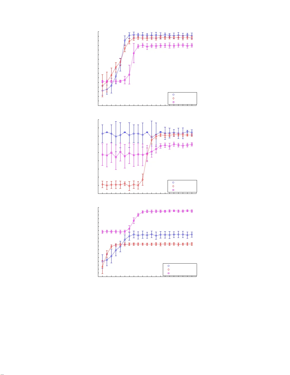
On Kernelizing Mahalanobis Dist ance Learning Algorithms On Kernelizing Mahalanobis Distance Learning Algorithms Ratthac hat Chatpatanasiri ra ttha cha t.c@student.chula.ac.th T eesid Korsrilabutr g48tkr@cp.eng.chula.ac.th P a sakorn T angc hanachaianan p asak orn.t@student.chula. ac.th Bo onserm Kijsirikul boonserm.k@chula.ac.th Dep artment of Computer E ngine ering, Chulalongkorn University, Pa thumwan, Bangkok, Thaila nd. Abstract This pap er fo cuses on the problem of kernelizing an existing sup ervised Ma ha lanobis distance learner. The following features are included in the paper . Firstly , three p opular learners, namely , “neig h b orho o d comp onent a nalysis”, “larg e margin near est neigh b ors” and “disc r iminant neighborho o d em be dding ” , whic h do not ha ve kernel versions a re ker- nelized in order to impro ve their classification perfor mances. Seco ndly , an alternative ker- nelization framew ork called “KPCA tric k” is presented. Implemen ting a learner in the new framework gains several adv ant ages ov er the standard framework, e.g. no mathematical formulas and no reprog ramming are required for a kernel implemen tation, the framework av oids troublesome problems such as singularity , etc. Thirdly , while the truths of repre- senter theor ems are just assumptions in previo us pap ers related to ours, here, r epresenter theorems are for mally proven. The proo fs v alidate b oth the kernel trick and the KPCA trick in the context of Mahalanobis distance learning. F ourthly , unlike pre v ious works which a lwa y s apply brute force metho ds to select a kernel, w e inv estigate tw o approaches which c an b e efficiently adopted to co nstruct an a ppr opriate k ernel for a given dataset. Finally , numerical re s ults o n v arious real-world datasets are presented. 1. In tro duction Recen tly , man y Mahalanobis distance learners are inv ent ed (Chen et al., 2005; Go ldb erger et al., 2005; W einb erger et al., 2006; Y ang et al., 2006; Su giy ama, 2006; Y an et al., 2007; Zhang et a l., 2007; T orresani & Lee , 2007; Xing e t al., 2003). These recen tly prop osed learners are carefully designed so that th ey can hand le a class of p r oblems where data of one class form m u lti-mod alit y where classical learners suc h as pr in cipal comp onen t analysis (PCA) and Fisher discriminan t analysis (FD A) cannot hand le. T herefore, promisingly , the new learners usually o utp erf orm the classic al learners o n exp erimen ts reported in recen t pap ers. Nev ertheless, s in ce learning a Mahalanobis distance is equiv alen t to learning a linear map, the inabilit y to learn a n on-linear transformation is one imp ortan t limitat ion of all Mahalanobis distance learners. As the researc h in Mahalanobis d istance learning has just recen tly b egun, sev eral issues are left op en such as (1) some efficient learners d o not ha ve non-linear extensions, (2) the k ernel trick (Sch¨ olk opf & Smola, 2 001), a standard non-linearization method, is not fully automa tic in the sense that new mathematical formula s ha v e to b e d eriv ed and new programming co des hav e to b e implemente d; th is is not con v enien t to non-exp erts, (3) existing algorithms “assume” the truth of the r epr esenter the or em (Sc h¨ olko pf & S mola, 2001, Chapter 4); ho w ev er, to our kno wledge, there is no formal pro of of the theorem in the con text of Mahalanobis distance learning, and (4) the problem of ho w to select an efficien t 1 Cha tp a t anasiri, K orsrilabutr, T angchanachaianan & Kijsirikul k ernel f unction has b een left unt ouc hed in pr evious w orks; curr ently , the b est kernel is ac hieved via a b rute-force m etho d such as cross v alidation. In this p ap er, w e highlight the follo w ing ke y con tributions: • T h ree p opular le arners recen tly prop osed in the lit eratures, n amely , neighb orho o d c om- p onent analysis (NCA) (Goldb erger et al., 2005), lar ge mar gin ne ar est neighb ors (LMNN) (W ein b erger et al., 2006) and discriminant nei g hb orho o d emb e dding (DNE) (Z h ang et al., 2007) are ke rnelized in order to imp ro v e their classification p erformances with r esp ect to the kNN algorithm. • A KP CA trick framew ork is presen ted as an alt ernativ e c hoice to the k ernel-tric k framew ork. In contrast to the kernel trick, the K PCA tric k d o es n ot require users to deriv e new mathematical form ulas. A lso, whenev er an implementa tion of an o riginal learner is a v ailable, users are not required to re-implemen t the k ern el versio n of the original learner. Moreo ve r, t he new framework a vo ids problems suc h as sin gularit y in eigen-decomposition and pro vides a conv enien t wa y to sp eed up a learner. • Tw o represen ter theorems in the cont ext of Mahalanobis distance learning are prov en. Our theorems justify b oth the k ernel-tric k and the K PCA-tric k framew orks. Moreo v er, the theorems v alidate k ern elized algo rithms learning a Mahalanobis distance in any separable Hilb ert s p ace and also co v er kernelize d algorithms p erformin g dimensionalit y reduction. • The prob lem of efficien t kernel sel ection is dealt with. Firstly , we in v estigat e the kernel alignment method prop osed in p revious w orks (Lanckriet et al., 2004 ; Zh u et al., 2005) to see whether it is appropriate for a ke rnelized Mahalanobis distance learner or not. Sec ondly , w e inv estigate a simp le method wh ic h constructs an unw eigh ted com bination of base k ernels. A theoretical result is provided to s u pp ort this simple approac h. Kernel constructions based on our t w o approac hes require m uc h shorter run ning time wh en comparing to the standard cross v alidatio n approac h. • As kNN is already a non-linear classifier, th ere are some doubts ab out the usefulness of k ernelizing Mahalanobis distance learners (W ein b erger et al., 200 6, pp. 8). W e pro- vide an explanation and conduct extensiv e exp erimen ts on real-w orld datasets to prov e the usefulness of th e k ernelization. 2. Bac kground Let { x i , y i } n i =1 denote a trainin g set of n lab eled examples with inp uts x i ∈ R D and cor- resp onding class lab els y i ∈ { c 1 , ..., c p } . Any Mahala nobis distance can b e represen ted b y a sym metric p ositiv e s emi-defin ite (PSD) matrix M ∈ S D + . Here, w e denote S D + as a space of D × D PSD matrices. Giv en t w o p oin ts x i and x j , and a P SD matrix M , the Maha- lanobis distance with resp ect to M b et w een the t w o p oints is defined as || x i − x j || M = p ( x i − x j ) T M ( x i − x j ). Our goal is to find a PSD matrix M ∗ that minimizes a reasonable ob jectiv e function f ( · ): M ∗ = arg min M ∈ S D + f ( M ) . (1) Since the P S D matrix M c an b e decomp osed to A T A , w e can equiv alen tly restate our problem as learning the b est matrix A : A ∗ = arg min A ∈ R d × D f ( A ) . (2) 2 On Kernelizing Mahalanobis Dist ance Learning Algorithms Note that d = D in the s tand ard sett ing, b ut for the purp ose of dimensionalit y reduction w e can learn a low-rank p ro jection by restricting d < D . After learning the b est linear map A ∗ , it will b e used b y kNN to compute the distance b et ween t w o p oin ts in the transform ed space as ( x i − x j ) T M ∗ ( x i − x j ) = || A ∗ x i − A ∗ x j || 2 . In th e follo wing subsections, three p opular algorithms, w hose ob jectiv e functions are mainly designed for a further use of kNN classification, are presen ted. Despite their ef- ficiency and p opularit y , the three algorithms do not ha v e the ir k ernel versions, and th us in this pap er we are primarily in terested in kerneliz ing these three algorithms in order to impro v e their classificatio n p erf ormances. 2.1 Neighborho o d Comp onent Analysis (NCA) Algorithm The original goal of NCA (Goldb erger et al., 2005 ) is to optimize th e le ave- one- out (LOO) p erformance on training data. Ho wev er, as the actual LOO classification error of kNN is a non-smo oth function of the matrix A , Goldb erger et al. prop ose to m inimize a sto chast ic v arian t of the LO O kNN score which is defined as follo ws: f N C A ( A ) = − X i X y j = c i p ij , (3) where p ij = exp( −|| A x i − A x j || 2 ) P k 6 = i exp( −|| A x i − A x k || 2 ) , p ii = 0 . Optimizing f N C A ( · ) can be d one b y applying a gradien t b ased metho d. On e ma jor disad- v an tage of NCA, ho wev er, is that f N C A ( · ) is not conv ex, and the gradien t based metho ds are th us prone to lo cal optima. 2.2 Large Margin N earest Neigh b or (LMNN) Algorithm In L MNN (W einberger et al., 2006), the output Mahalanobis dista nce is optimized w ith the goal that for e ach p oint, its k-ne ar est neighb ors always b elong to the same class while examples fr om differ ent classes ar e sep ar ate d by a lar ge mar gin . F or eac h p oin t x i , we d efine its k tar get neighb ors as the k ot her inputs w ith the same lab el y i that are closest to x i (with respect to the Euclidean distance in the inpu t space). W e use w ij ∈ { 0 , 1 } to indicate whether an input x j is a target neigh b or of an inp ut x i . F o r con venience, w e define y ij ∈ { 0 , 1 } to indicate whether or n ot the lab els y i and y j matc h. The ob jectiv e fu nction of LMNN is as follo ws: f LM N N ( M ) = X i,j w ij || x i − x j || 2 M + c X i,j,l w ij (1 − y il )  1 + || x i − x j || 2 M − || x i − x l || 2 M  + , where [ · ] + denotes the standard hinge loss: [ z ] + = max ( z , 0). The term c > 0 is a p ositiv e constan t typica lly set by cross v alidatio n. The ob jectiv e function ab o ve is con vex 1 and has 1. There is a vari ation on LMNN called “la rge margin component analysis” (LMCA) (T orresani & Lee, 2007) whic h prop oses to optimize A instead of M ; h o we ver, LMCA d o es n ot preserve some desira ble prop erties, such as con vexit y , of LMNN , and therefore the algorithm “Kernel LMCA” presented th ere is different from “Kernel LMNN” presented in t h is pap er. 3 Cha tp a t anasiri, K orsrilabutr, T angchanachaianan & Kijsirikul t wo co mp eting terms. Th e first term p enalizes large distances b et ween eac h input and its target neigh b ors, w h ile the second term p enalizes small distances b et wee n eac h in p ut and all other in p uts that do not share the same lab el. 2.3 Discriminan t N eigh b orho o d Embedding (DNE) Algorithm The main id ea of DNE (Zhang et al., 200 7) is quite similar to LMNN. DNE seeks a linear transformation such that neighborh o o d p oin ts in the same cl ass are squeezed but those in differen t classes are separated as muc h as p ossible. Ho wev er, DNE do es not care ab out the notion of margin; in the case of LMNN, w e wa nt ev ery p oin t to stay f ar from p oin ts of other classes, b ut for DNE, we w an t the a v erage distance b et ween tw o neigh b orho o d p oints of differen t classes to b e large. Another difference is that LMNN can learn a full Mahalanobis distance, i.e. a general weighte d linear pro jection, wh ile DNE can lea rn only an unweighte d linear pro jection. Similar to L MNN, we define two se ts of k target neigh b ors for eac h p oin t x i based on the Euclidean distance in th e input space. F or eac h x i , let N eig I ( i ) b e the set of k n earest neigh b ors ha ving the same lab el y i , and let N eig E ( i ) b e the set of k nearest neigh b ors ha ving differen t lab els f r om y i . W e define w ij as follo ws w ij =      +1 , if j ∈ N eig I ( i ) ∨ i ∈ N eig I ( j ) , − 1 , if j ∈ N eig E ( i ) ∨ i ∈ N eig E ( j ) , 0 , otherwise . The ob jectiv e fu nction of DNE is: f D N E ( A ) = X i,j w i,j || A x i − A x j || 2 . whic h can b e reform ulated (up to a constan t factor) to b e f D N E ( A ) = trace( AX ( D − W ) X T A T ) , where W is a symmetric matrix with elemen ts w ij , D is a d iagonal matrix with D ii = P j w ij and X is the matrix of input p oints ( x 1 , ..., x n ). It is a w ell-kno w n result f rom sp ectral graph theory (v on Luxbu rg, 2007) that D − W is symmetric but is not necessarily PSD. T o solv e the problem b y eigen-decomp osition, the constrain t AA T = I is added (recall that A ∈ R d × D ( d ≤ D )) so that we h a ve the follo wing optimization problem: A ∗ = arg min AA T = I trace( AX ( D − W ) X T A T ) . (4) 3. Kernelization In this sect ion, w e fo cus on t wo k ern elizat ion f r amew orks going to non-linea rize the three algorithms pr esen ted in the previous section. First, the standard kernel trick framewo rk is presen ted. Next, the KPCA trick framew ork whic h is an alternativ e to the k ernel- tric k f ramew ork is presen ted. Kernelization in this new f r amew ork is con ve nient ly don e with an application of kernel pr incip al c omp onent analysis (KPCA). Finally , repr esen ter 4 On Kernelizing Mahalanobis Dist ance Learning Algorithms theorems are pr o ven to v alidate all applicatio ns of the t wo k ern elizat ion fr amew orks in the con text of Mahal anobis distance learning. Note that in some p revious w orks (Chen et al. , 2005; Glob erson & Row eis, 2006; Y an et al., 2007 ; T orr esani & Lee, 2007 ), the v alidit y of applications of the the k ernel tric k has not b een pro v en. 3.1 Historical Bac kground After finishing wr iting the current pap er, w e just knew that this n ame was fi rst app eared in the pap er of Chap elle and Sch¨ olk opf (2001) wh o first applied this metho d to inv arian t supp ort v ector mac hines; moreo ver, it is app eared t o us that the KPCA trick has been kno wn t o some researc h ers (priv ate comm unication t o some ECML review ers). Wit hout kno wing ab out this fact, we reinv ent ed the framew ork and, coinciden tally , called it “KPCA tric k” our selv es. Nev ertheless, w e will sho wn in Section 5.1 that, in the con text of Maha- lanobis distance learning, the KPCA tric k non-trivially has many adv an tages ov er the k ernel tric k; we b eliev e that this consequence is new and is not a consequence of previous w orks. Also, mathematical to ols pr o vid ed in previous w orks (Sch¨ olk opf & Smola, 2001; Ch ap elle & Sch¨ olk opf, 2001) are not en ou gh to pro v e the v alidit y of the KPC A tric k in this con text, and th us the new v alidation pr o of of the KPCA trick is needed (see our Th eorem 1). 3.2 The Kernel-T ric k F ramew ork Giv en a PSD k ern el function k ( · , · ) (Sc h¨ olk opf & Smola, 2001), w e denote φ , φ ′ and φ i as mapp ed data (in a feature sp ace asso ciated with th e k ern el) of eac h example x , x ′ and x i , resp ectiv ely . A (squared) Mahalanobis distance under a matrix M in the feature space is ( φ i − φ j ) T M ( φ i − φ j ) = ( φ i − φ j ) T A T A ( φ i − φ j ) . (5) T o b e co nsistent w ith Subsection 2.3, let A T = ( a 1 , ..., a d ). Denote a (p ossibly i nfin ite- dimensional) m atrix of the mapp ed training data Φ = ( φ 1 , ..., φ n ). The main i dea of th e k ernel-tric k framew ork is to parameterize (see represent er theorems b elo w) A T = Φ U T , (6) where U T = ( u 1 , ..., u d ). Substituting A in Eq. (5) b y u sing Eq. (6), we ha v e ( φ i − φ j ) T M ( φ i − φ j ) = ( k i − k j ) T U T U ( k i − k j ) , where k i = Φ T φ i =  h φ 1 , φ i i , ..., h φ n , φ i i  T . (7) No w our form ula dep ends only on an inner-pro duct h φ i , φ j i , and th us the k ernel trick can b e no w applied by usin g the fact th at k ( x i , x j ) = h φ i , φ j i for a PSD kernel fun ction k ( · , · ). Therefore, the problem of finding the b est Mahalanobis distance in the feature space is n o w reduced to fin ding the b est linear t ransformation U of siz e d × n . Nonetheless, it often happ ens that finding U is muc h more troublesome than findin g A in the input space, ev en their optimization p roblems lo ok similar, as sho wn in Section 5.1. Once w e find the mat rix U , the Mahal anobis distance from a new test p oin t x ′ to an y input p oin t x i in the feature sp ace can b e calculated as follo ws: || φ ′ − φ i || 2 M = ( k ′ − k i ) T U T U ( k ′ − k i ) , (8) 5 Cha tp a t anasiri, K orsrilabutr, T angchanachaianan & Kijsirikul where k ′ = ( k ( x ′ , x 1 ) , ..., k ( x ′ , x n )) T . kN N classification in the feat ure space can b e p er- formed based on Eq. (8). 3.3 The KPCA-T ric k F ramew ork As w e emphasize ab o v e, although the ke rnel tric k framew ork can b e applied to non-linearize the three learners int ro du ced in S ection 2, it often happ ens that finding U is muc h more troublesome than finding A in th e inp ut sp ace, ev en their optimization pr oblems lo ok similar (see S ection 5.1). In this section, w e d evelo p a KPCA trick framew ork whic h can b e muc h more con v en iently applied to kernelize the three learners. Denote k ( · , · ), φ i , φ and φ ′ as in Subsection 3.2. The cen tral idea of the KPCA tric k is to represen t eac h φ i and φ ′ in a new “finite”-dimensional sp ace, w ithout any loss of information. Within the framewo rk, a new co ordinate of eac h example is computed “explici tly”, and eac h example in the new co ordin ate is then u s ed as the inpu t of any existing Mahalanobis distance learner. As a result, by using the KPCA tric k in place of the ke rnel tric k, there is no need to deriv e new mathematical formulas and no need to implement new algorithms. T o simplify the discussion of KPC A, w e assume that { φ i } is linea rly indep enden t and has its cen ter at the origin, i.e. P i φ i = 0 (o therwise, { φ i } can b e cente red b y a simp le pre-pro cessing step (Sha we-T a ylor & Cr istianini, 2004, p. 115)). Since w e ha v e n total examples, the span of { φ i } h as dimensionalit y n . Here w e claim that eac h example φ i can b e represen ted as ϕ i ∈ R n with resp ect to a new orthono rmal basis { ψ i } n i =1 suc h that span ( { ψ i } n i =1 ) is the same as span ( { φ i } n i =1 ) without loss of an y information. Mo re precisely , w e define ϕ i =  h φ i , ψ 1 i , . . . , h φ i , ψ n i  = Ψ T φ i . (9) where Ψ = ( ψ 1 , ..., ψ n ). Not e that a lthough w e ma y be unable to n umerically represen t eac h ψ i , a n inner-p r o duct of h φ i , ψ j i can b e conv enient ly co mputed by K PCA (or k ernel Gram-Sc h midt (Sha w e-T a ylor & Cristianini, 2004)) . Lik ewise, a new test p oint φ ′ can b e mapp ed to ϕ ′ = Ψ T φ ′ . C onsequen tly , the mapp ed data { ϕ i } and ϕ ′ are finite-dimensional and can b e explicitly computed. 3.3.1 The KPCA-trick Algorith m The KP CA-tric k algorit hm consisting o f three simple steps is sho wn in Figure 1. NCA, LMNN, DN E and other learners, including t hose in other setti ngs (e.g. semi-sup ervised settings), wh ose k ernel ve rsions are previously unknown (Y ang et al., 2006; Xing et al. , 2003; Chatpatanasiri & Kijsirikul, 2008) can all b e k ernelized b y this simple algo rithm. Therefore, it is m uc h more con v enien t to ke rnelize a learner by applying the KPCA-tric k framew ork rather than applying the k ernel-tric k framewo rk. In the algorithm, w e d enote a Mahalanobis distance learner by maha whic h p erforms the op timization pro cess sho wn in Eq. 1 (or Eq. 2) and outputs the b est Mahalanobis distance M ∗ (or the b est linear map A ∗ ). 3.3.2 Rep resenter Theorems Is it v alid to repr esen t an infin ite-dimensional ve ctor φ b y a fin ite-dimensional v ector ϕ ? In the con text of SVMs (Chap elle & Sc h¨ olk opf, 2 001), this v alidit y of the KPCA tric k is 6 On Kernelizing Mahalanobis Dist ance Learning Algorithms Input: 1. training examples: { ( x 1 , y 1 ) , ..., ( x n , y n ) } , 2. new example: x ′ , 3. k ern el function: k ( · , · ) 4. Mahalanobis distance learning algorithm: maha Algorithm: (1) App ly kp ca ( k , { x i } , x ′ ) su c h that { x i } 7→ { ϕ i } and x ′ 7→ ϕ ′ . (2) App ly maha with new in puts { ( ϕ i , y i ) } to ac hiev e M ∗ or A ∗ . (3) Perform kNN based on the distance || ϕ i − ϕ ′ || M ∗ or || A ∗ ϕ i − A ∗ ϕ ′ || . Figure 1: The KPC A-tric k algorithm. easily achie v ed by straigh tforw ardly extending a pro of of an established repr esenter theorem (Sc h¨ olk opf et al., 2001) 2 . In the cont ext of Mahalanobis distance learning, ho wev er, p ro ofs pro vided in previous wo rks cannot b e directly extended. Note that, in the SVM cases considered in previous w orks, what is learned is a hyp erplane, a linear functional outpu tting a 1-dimensional v alue. In our case , as sho wn in Eq. 6, what is learned is a linear map whic h, in general, ou tp u ts a c ountably infinite dimensional v ector. Hence, to pro v e the v alidit y of the K P C A tric k in our case, w e need some mathematic al to ols whic h can handle a count ably infinite dimensionalit y . Belo w w e giv e our ve rsions of represent er theorems whic h pr ov e the v alidit y of the KPCA tric k in the curren t con text. By our r epresen ter theorems, it is the f act t hat, g iv en an ob jectiv e fu nction f ( · ) (see Eq. (1)), the optimal v alue of f ( · ) based on the input { φ i } is equal to the optimal v alue of f ( · ) based on the inp ut { ϕ i } . Hence, the repr esentat ion of ϕ i can b e safely app lied. W e separate the p roblem of Mahalanobis distance learning in to tw o differen t cases. The fi rst theorem co vers Mahalanobis d istance learners (learning a fu ll-rank linear transformation) while the second theorem co ve rs d imensionalit y reduction algorithms (learning a lo w-ran k linear transformation). Theorem 1. (F ul l-R ank R epr esenter The or em) L et { ˜ ψ i } n i =1 b e a set of p oints in a fe atur e sp ac e X such that span ( { ˜ ψ i } n i =1 ) = span ( { φ i } n i =1 ) , and X and Y b e sep ar able Hilb ert sp ac es. F or an obje ctive function f dep ending only on {h Aφ i , Aφ j i} , the optimiza tion min A : f ( h Aφ 1 , Aφ 1 i , . . . , h Aφ i , Aφ j i , . . . , h Aφ n , Aφ n i ) s.t. A : X → Y is a b ounde d line ar map , has th e same optimal value as, min A ′ ∈ R n × n f ( ˜ ϕ T 1 A ′ T A ′ ˜ ϕ 1 , . . . , ˜ ϕ T i A ′ T A ′ ˜ ϕ j , . . . , ˜ ϕ T n A ′ T A ′ ˜ ϕ n ) , wher e ˜ ϕ i =  h φ i , ˜ ψ 1 i , . . . , h φ i , ˜ ψ n i  T ∈ R n . 2. A representer theorem, along with Mercer theorem, is a key ingredient for v alidating the kernel tric k (Sch¨ olk opf & Smola, 2001). The origin of the class ical representer theorem is dated b ac k to at lea st 1970s (Kimeldorf & W ahba, 1971 ). 7 Cha tp a t anasiri, K orsrilabutr, T angchanachaianan & Kijsirikul T o our kno w ledge, mathematical to ols pro vid ed in the work o f Sc h¨ olk opf and Smola (2001 , Chapter 4) are not enough to prov e Th eorem 1. The pr o of pr esen ted h ere is a non- straigh tforward extension of Sc h¨ olko pf and Smola’s w ork. W e also n ote that Theorem 1, as w ell as Theorem 2 sho wn b elo w, is more general than what w e discuss ab ov e. Th ey justify b oth the kernel tric k (by sub stituting ˜ ψ i = φ i and hence ˜ ϕ i = k i ) and the KPCA tric k (b y substituting ˜ ψ i = ψ i and hence ˜ ϕ i = ϕ i ). T o start pro ving Theorem 1, the follo wing lemma is useful. Lemma 1. L et X , Y b e two Hilb ert sp ac es and Y is sep ar able, i .e. Y h as a c ountable orthono rmal b asis { e i } i ∈ N . A ny b ounde d line ar map A : X → Y c an b e uniquely de c omp ose d as P ∞ i =1 h· , τ i i X e i for some { τ i } i ∈ N ⊆ X . Pr o of. As A is b ounded, the linear functional φ 7→ h Aφ, e i i Y is b ounded f or ev ery i since, b y Cauc hy-Sc hw arz inequalit y , |h Aφ, e i i Y | ≤ || Aφ |||| e i || ≤ || A |||| φ || . By Riesz represen tation theorem, the map h A · , e i i Y can b e w r itten as h· , τ i i X for a unique τ i ∈ X . Since { e i } i ∈ N is an orthonorm al b asis of Y , for ev ery φ ∈ X , Aφ = P ∞ i =1 h Aφ, e i i Y e i = P ∞ i =1 h φ, τ i i X e i . Pr o of. (Theorem 1) T o a voi d complicated notat ions, we omit subscripts such as X , Y of inner p ro ducts. The pro of will co nsist of t w o steps. In t he first step, w e will pro v e the theorem b y assuming that { ˜ ψ i } n i =1 is an orthonormal set. In the second step, we prov e the theorem in general cases wh ere { ˜ ψ i } n i =1 is not necessarily orthonorm al. The p ro of of th e first step r equ ir es an application of F ubini theorem (Lewkee ratiyutkul, 2006). Step 1 . Assum e that { ˜ ψ i } n i =1 is an orthonormal set. Let { e i } ∞ i =1 b e an orthonormal basis of Y . F or an y φ ′ ∈ X , w e ha v e, by Lemma 1, Aφ ′ = P ∞ k =1 h φ ′ , τ k i e k . Hence, for eac h b ounded linear map A : X → Y , and φ, φ ′ ∈ span ( { ˜ ψ i } n i =1 ), we ha v e h Aφ, Aφ ′ i = P ∞ k =1 h φ, τ k ih φ ′ , τ k i . Note that E ach τ k can b e decomp osed as τ ′ k + τ ⊥ k suc h that τ ′ k lies in span ( { ˜ ψ i } n i =1 ) and τ ⊥ k is orthogonal to the span. Th ese facts mak e h φ ′ , τ k i = h φ ′ , τ ′ k i for every k . Moreo ver, τ ′ k = P n j = 1 u k j ˜ ψ j , for s ome { u k 1 , ..., u k n } ⊂ R n . Hence, we ha v e h Aφ, Aφ ′ i = ∞ X k =1 h φ, τ k ih φ ′ , τ k i = ∞ X k =1 h φ, τ ′ k ih φ ′ , τ ′ k i = ∞ X k =1 h φ, n X i =1 u k i ˜ ψ i ih φ ′ , n X i =1 u k i ˜ ψ i i = ∞ X k =1 n X i,j =1 u k i u k j h φ, ˜ ψ i ih φ ′ , ˜ ψ j i (F ubini theorem: explained b elo w) = n X i,j =1 ∞ X k =1 u k i u k j ! h φ, ˜ ψ i ih φ ′ , ˜ ψ j i = n X i,j =1 G ij h φ, ˜ ψ i ih φ ′ , ˜ ψ j i = ˜ ϕ T G ˜ ϕ ′ = ˜ ϕ T A ′ T A ′ ˜ ϕ ′ . A t the fourth equalit y , we app ly F ub ini theorem to sw ap the t wo summ ations. T o see that F ubini theorem can b e applied at the fourth equalit y , w e first note that P ∞ k =1 u 2 k i is finite 8 On Kernelizing Mahalanobis Dist ance Learning Algorithms for eac h i ∈ { 1 . . . n } since ∞ X k =1 u 2 k i = ∞ X k =1 h ˜ ψ i , n X j = 1 u k j ˜ ψ j ih ˜ ψ i , n X j = 1 u k j ˜ ψ j i = || A ˜ ψ i || 2 < ∞ . Applying the ab o ve result together with Cauc hy-Sc hw arz inequalit y and F ubini theorem for non-negativ e summation, we hav e ∞ X k =1 n X i,j =1 | u k i u k j h φ, ˜ ψ i ih φ ′ , ˜ ψ j i| = n X i,j =1 ∞ X k =1 | u k i u k j h φ, ˜ ψ i ih φ ′ , ˜ ψ j i| = n X i,j =1 |h φ, ˜ ψ i ih φ ′ , ˜ ψ j i|  ∞ X k =1 | u k i u k j |  ≤ n X i,j =1 |h φ, ˜ ψ i ih φ ′ , ˜ ψ j i| v u u t  ∞ X k =1 u 2 k i  ∞ X k =1 u 2 k j  < ∞ . Hence, the su mmation con verges absolutely and thus F ubini theorem can b e applied as claimed ab o ve. Again, using the f act that P ∞ k =1 u 2 k i < ∞ , w e ha v e that eac h element of G , G ij = P ∞ k =1 u k i u k j , is finite. F urthermore, the matrix G is PSD since eac h of its elemen ts can b e regarded as an inner pro duct of t wo v ectors in ℓ 2 . Hence, w e finally h a ve that h Aφ i , Aφ j i = ˜ ϕ T i A ′ T A ′ ˜ ϕ j , for eac h 1 ≤ i, j ≤ n . Hence, whenev er a map A is giv en, we can construct A ′ suc h that it r esults in the same ob jectiv e function v alue. By rev ersing the pro of, it is easy to see that the conv erse is also tru e. The first step of the pro of is finished. Step 2 . W e n o w prov e the theorem without assuming that { ˜ ψ i } n i =1 is an orthonormal set. Let all notations b e the same as in Step 1. Let Ψ ′ b e the matrix ( ˜ ψ 1 , ..., ˜ ψ n ). Define { ψ i } n i =1 as an orthonormal set such that span ( { ψ i } n i =1 ) = s pan ( { ˜ ψ i } n i =1 ) and Ψ = ( ψ 1 , ..., ψ n ) and ϕ i = Ψ T φ i . Then, w e ha v e that ˜ ψ i = Ψ c i for some c i ∈ R n and Ψ ′ = Ψ C where C = ( c 1 , ..., c n ). Moreo ver, since C map from an ind ep endent set { ψ i } to another indep endent set { ˜ ψ i } , C is inv ertible. W e then ha v e, for an y A ′ , ˜ ϕ T i A ′ T A ′ ˜ ϕ j = φ T i Ψ ′ A ′ T A ′ Ψ ′ T φ j = φ T i Ψ C A ′ T A ′ C T Ψ T φ j = ϕ T i C A ′ T A ′ C T ϕ j = ϕ T i B T B ϕ j , where A ′ C T = B and A ′ = B ( C T ) − 1 . Hence, for an y B w e h a ve the matrix A ′ whic h giv es ˜ ϕ T i A ′ T A ′ ˜ ϕ j = ϕ T i B T B ϕ j . Using the s ame arguments as in Step 1, w e fin ish the p ro of of Step 2 and of Theorem 1. Theorem 2. (L ow-R ank R epr esenter The or em) Define { ˜ ψ i } n i =1 and ˜ ϕ i b e as in The or em 1. an obje ctive function f dep ending only on {h Aφ i , Aφ j i} , the optimiza tion min A : f ( h Aφ 1 , Aφ 1 i , . . . , h Aφ i , Aφ j i , . . . , h Aφ n , Aφ n i ) s.t. A : X → R d is a b ounde d line ar map , 9 Cha tp a t anasiri, K orsrilabutr, T angchanachaianan & Kijsirikul has th e same optimal value as, min A ′ ∈ R d × n f ( ˜ ϕ T 1 A ′ T A ′ ˜ ϕ 1 , . . . , ˜ ϕ T i A ′ T A ′ ˜ ϕ j , . . . , ˜ ϕ T n A ′ T A ′ ˜ ϕ n ) . The pro of of Theorem 2 is a generaliza tion of the pro ofs in previous works (Sc h¨ olk opf & Smola, 2001, Chap. 4). Pr o of. (Theorem 2) Let { e i } d i =1 b e the canonical b asis of R d , and let φ ∈ span { ˜ ψ 1 , . . . ˜ ψ n } . By Lemm a 1, Aφ = P d i =1 h φ, τ i i e i for some τ 1 , . . . , τ d ∈ X . Eac h τ i can b e decomp osed as τ ′ i + τ ⊥ i suc h that τ ′ i lies in span { ˜ ψ 1 , . . . , ˜ ψ n } and τ ⊥ i is orthogonal to the s p an. These facts mak e h φ, τ i i = h φ, τ ′ i i for every i . W e then ha v e, for some u ij ∈ R , 1 ≤ i ≤ d, 1 ≤ j ≤ n , Aφ = d X i =1 h φ, n X j = 1 u ij ˜ ψ j i e i = d X i =1 e i n X j = 1 u ij h φ, ˜ ψ j i =    u 11 · · · u 1 n . . . . . . . . . u d 1 · · · u dn       h φ, ˜ ψ 1 i . . . h φ, ˜ ψ n i    = U ˜ ϕ . Since every φ i is in the sp an, we conclude that Aφ i = U ˜ ϕ i . No w , one can easily c hec k that h Aφ i , Aφ j i = ˜ ϕ T i U T U ˜ ϕ j . Hence, wheneve r a map A is giv en, we can construct U suc h that it results in the same ob jectiv e function v alue. By rev ersing the pro of, it is easy to see that the con verse is also true, and th us the theorem is pr o ven (by renaming U to A ′ ). Note that the pro of of Theorem 2 cannot b e directly used for pro ving Th eorem 1 (let d = ∞ and U ∈ R ∞× n , and Theorem 2 is still v alid. Ho w ev er, to practically b e useful, we need a finite-dimensional linear map. Hence, w e m ust show that U T U ∈ R n × n b y pro vin g that u ij < ∞ for all i, j ). 3.3.3 Rema rks 1. Note that by Mercer theorem (Sc h ¨ olk opf & S mola, 2001, p p . 37 ), w e can either think of eac h φ i ∈ ℓ 2 or φ i ∈ R N for some p ositiv e integ er N , and th u s the assump tion of Theorem 1 that X , as well as Y , is separable Hilb ert space is then v alid. Also, b oth theorems require that the ob jectiv e function of a learning algorithm m ust depend only on {h Aφ i , Aφ j i} n i,j =1 or e quiv alen tly {h φ i , M φ j i} n i,j =1 . This c ondition is, actually , not a strict condition since learners in lite ratures ha ve their ob jectiv e functions in this form (Chen et al., 2005; Gold- b erger et al., 2005; Glob erson & Row eis, 2006; W ein b erger et al., 20 06; Y ang et al., 2006; Sugiy ama, 2006 ; Y an et al., 2007; Zhang et al., 2007; T orresani & Lee, 2007). 2. No te th at the t w o theorems stated in this section do not require { ˜ ψ i } to b e an or- thonormal set. How ev er, there is an adv an tage of the KPCA tric k whic h restricts ˜ ψ i = ψ i as in E q. (9); this will b e discussed in S ect. 5.1. 3. A running time of eac h learner strongly dep end s o n the dimensionalit y of the inpu t data. As recommended by W ein b erger et al. (2006), it can b e helpful to first app ly a di- mensionalit y r ed u ction algorithm suc h as PCA b efore p erforming a learning pro cess: the learning pro cess can be tremendously sp eed up b y retaining only , says, the 200 largest- v ariance pr in cipal comp onen ts of the in p ut data. In the KPC A tric k framework illustrated 10 On Kernelizing Mahalanobis Dist ance Learning Algorithms in Figure 1, dimensionalit y reduction can b e p erformed w ithout an y extra w ork as KPCA is already applied at the first place. 4. The stronger v ersion of Theorem 2 can b e ac hiev ed b y ins erting a regularizer into the ob jectiv e function of a (k ernelized) Mahalanobis distance learner as stated in Theorem 3. F or compact notations, w e use the fact that A is rep r esen table by { τ i } as sho wn in Lemm a 1. Theorem 3. (Str ong R epr esenter The or em) Define { ˜ ψ i } n i =1 and f b e as in The or em 1. F or monoton ic al ly incr e asing functions g i , let h ( τ 1 , ..., τ d , φ 1 , ..., φ n ) = f ( h τ 1 , φ 1 i , . . . , h τ i , φ j i , . . . , h τ n , φ d i ) + d X i =1 g i ( || τ i || ) . Any optimal set of line ar functionals arg min { τ i } h ( τ 1 , ..., τ d , φ 1 , ..., φ n ) s.t. ∀ i τ i : X → R is a b ounde d line ar functional must admit the r epr esentation of τ i = P n j = 1 u ij ˜ ψ j ( i = 1 , . . . , d ) . The pro of of this result is v ery similar to that of (Sc h¨ olk opf & Smola, 2001, Th eorem 4.2) so that w e omit its detail s here. In fact, to pro v e the v alidation of KDNE, we need this strong represen ter theorem (see the case of KPCA in Sch¨ olk opf and Smola (2001, pp.92)). T o apply Theorem 3 to our framew ork, w e can simply view A = ( τ 1 , ..., τ d ) T . If eac h g i is the squ are fu nction, th en regularizer b ecomes P d i =1 || τ i || 2 = || A || H S where || · || H S is the Hilb ert-Sc hmidt (HS) norm of an op erator. If eac h τ i is fin ite-dimensional, the HS norm is redu ced to the F rob enius norm || · || F . Here, w e allo w the HS norm of a b ounded linear op erator to take a v alue of ∞ . F or the k ernel tric k (by substituting ˜ ψ i = φ i ), the result ab o v e stat es that any optimal { τ i } must b e represen ted b y { Φ u i } . Th erefore, using the same notation as Su bsection 3.2, we ha v e d X i =1 g i ( || τ i || ) = d X i =1 || τ i || 2 = d X i =1 u T i Φ T Φ u i = d X i =1 u T i K u i = trace  U K U T ) . This regularizer is first app eared in the work of Glob erson and Row eis (20 06). Similarly , for the KPCA tric k (b y substituting ˜ ψ i = ψ i ), an y optimal { τ i } m ust b e represen ted by { Ψ u i } and, using the fact that Ψ T Ψ = I , we ha v e P d i =1 || τ i || 2 = trace  U U T ) = || U || 2 F . By adding the regularizer, trace( U K U T ) or || U || 2 F , int o existing ob jectiv e functions, w e ha v e a new class of le arners, namely , r e gularize d M ahalanobis distanc e le arners suc h as regularized KNCA (RKNCA), regularized KLMNN (RKLMNN) and regularized KDNE (RKDNE). Our framew ork can b e further extended in to a pr oblem in semi-sup ervised set- tings b y add in g more complicated functions of g i ( · ) suc h as manifold r e g u larizers , see e.g. Chatpatanasiri and Kijsirikul (200 8). W e plan to in vestig ate effect s of using v arious t yp es of regularizers in the near futur e. 11 Cha tp a t anasiri, K orsrilabutr, T angchanachaianan & Kijsirikul 4. Selection of a Kernel F unction The problem of s electi ng an effici en t kernel f unction is cen tral to all k ernel mac hines. Al l previous w orks on Mahala nobis distance learners use exhaustive m etho d s suc h as cross v alidation to s elect a k ernel function. In this section, we inv estigate a p ossibilit y to auto- maticall y construct a ke rnel whic h is app ropriate for a Mahalanobis distance learner. In the first part of this section, we consider a p opular metho d calle d kernel alignment (Lanc kr iet et al., 2004; Zh u et al., 2005 ) wh ic h is able to learn, f r om a t raining set, a k ernel in the form of k ( · , · ) = P i α i k i ( · , · ) where k 1 ( · , · ) , ..., k m ( · , · ) are pre-c hosen base k ernels. In the second p art of this section, we in v estigate a simple metho d whic h constru cts an un w eigh ted com b ination of base k ernels, P i k i ( · , · ) (henceforth refered to as an unweighte d ke rnel ). A theoretica l result is pro vided to supp ort this simp le approac h. Kernel co nstructions based on our t w o approac hes require m uc h shorter run ning time wh en comparing to the standard cross v alidatio n approac h. 4.1 Kernel Alignment Here, our k ernel alignment form ulation b elongs to the class of quadr atic programs (QPs) whic h can b e solv ed m ore effici en tly than the form ulations prop osed by Lanckriet e t al. (2004 ) and Zh u et al. (200 5) whic h b elong to the cla ss of semidefinite programs (SDPs) and quadratically constrained quadratic programs (QCQPs), resp ectiv ely (Bo yd & V an- den b erghe, 2004). T o use k ernel alignment in classification problems, the follo wing assumption is cen tral: for eac h couple of examples x i , x j , the id eal ke rnel k ( x i , x j ) is Y ij (Guermeur et al., 2004 ) where Y ij = ( +1 , if y i = y j , − 1 p − 1 , otherwise , and p is the num b er of classes in the training d ata. Denoting Y as the matrix ha ving elemen ts of Y ij , we then define the alignment b et ween the k ernel matrix K and the ideal k ernel matrix Y as follo ws: align( K, Y ) = h K, Y i F || K || F || Y || F , (10) where h· , ·i F denotes the F rob enius inn er-p ro duct s u c h that h K, Y i F = trace( K T Y ) and || · || F is the F rob enius norm indu ced by the F rob enius inner-p r o duct. Assume that w e h a ve m k ernel fu nctions, k 1 ( · , · ) , ..., k m ( · , · ) and K 1 , ..., K m are their corresp onding Gram matrice s with resp ect to the training data. I n this pap er, the k ernel function obtained from the alignmen t metho d is parameteriz ed in the form of k ( · , · ) = P i α i k i ( · , · ) where α i ≥ 0. Note that the obtained kernel function is guaran teed to b e p ositiv e semidefinite. In order to learn the b est co efficien ts α 1 , ..., α m , we solv e the f ollo wing optimizatio n problem: { α 1 , ..., α m } = arg max α i ≥ 0 align( K, Y ) , (11) where K = P i α i K i . Note that as K and Y are PSD, h K, Y i F ≥ 0. Since b oth the n umerator and denominator terms in the alignmen t equation can b e arbitrary large , w e can 12 On Kernelizing Mahalanobis Dist ance Learning Algorithms simply fix th e numerator to 1. W e then reformulate the problem as follo ws: arg max α i ≥ 0 , h K,Y i F =1 align( K, Y ) = arg min α i ≥ 0 , h K,Y i F =1 || K || F || Y || F = arg min α i ≥ 0 , h K,Y i F =1 || K || 2 F = arg min α i ≥ 0 , P i α i h K i ,Y i F =1 X i,j α i α j h K i , K j i F . Defining a PSD m atrix S whose elemen ts S ij = h K i , K j i F , a v ector b = ( h K 1 , Y i F , ..., h K m , Y i F ) T and a v ector α = ( α 1 , ..., α m ) T , w e then reform ulate Eq. (11) as follo ws: α = arg min α i ≥ 0 , α T b =1 α T S α . (12) This optimization problem is a Q P and can b e efficient ly solve d (Bo yd & V anden b erghe, 2004) ; hence, we are able to learn the b est k ernel function k ( · , · ) = P i α i k i ( · , · ) efficien tly . Since the magnitudes of the optimal α i are v aried du e to || K i || F , it is conv enien t to use k ′ i ( · , · ) = k i ( · , · ) / || K i || F and hence K ′ i = K i / || K i || F in the d eriv ation of Eq. (12). W e define S ′ and b ′ similar to S and b except that they are based on K ′ i instead of K i . Let γ = arg min γ i ≥ 0 , γ T b ′ =1 γ T S ′ γ . (13) It is easy to see that the fin al kernel fu nction k ( · , · ) = P i γ i k ′ i ( · , · ) achiev ed from Eq. (1 3) is n ot changed fr om the kernel ac h iev ed from Eq. (12). Note that w e can fur th er mo dify Eq. (12) to enforce sparseness of α and impro v e a sp eed of an algorithm by minimizing an upp er b ound of || K || F instead of minimizing the exact quan tit y so that the optimizat ion formula b elongs to the cla ss of linear programs (LPs) instead of QPs . min α i ≥ 0 , h K,Y i F =1 || K || F ≤ min α i ≥ 0 , h K,Y i F =1 || v ec ( K ) || 1 (14) where vec( · ) denotes a standard “v ec” o p erator con ve rting a matrix to a v ector (Mink a, 1997) . By using a standard trick for an absolute- v alued ob jectiv e fun ction (B o yd & V an- den b erghe, 200 4), Eq. (14) can b e solv ed b y linear p rogramming. Note that the ab o ve optimizatio n algorithm of minimizing the up p er b ound of a desired ob jectiv e function is similar to the p opular supp ort v ector mac hines where the hinge loss is minimize d instead of the 0/1 loss. 4.2 Un weigh ted Kernels In this sub section, we sho w th at a very simple ke rnel k ′ ( · , · ) = P i k i ( · , · ) is t heoretically efficien t, no less th an a ke rnel obtained from the alig nment metho d. De note φ k i as a mapp ed v ector of an original example x i b y a map asso ciated with a k ernel k ( · , · ). The main idea of the conte nt s p resen ted in this section is the follo wing simple bu t useful result. Prop osition 1. L et { α i } b e a set of p ositive c o efficie nts, α i > 0 for e ach i , and let k 1 ( · , · ) , ..., k m ( · , · ) b e b ase PSD kernels and k ( · , · ) = P i α i k i ( · , · ) and k ′ ( · , · ) = P i k i ( · , · ) . Then, ther e exists an invertible line ar map B such that B : φ k ′ i → φ k i for e ach i . 13 Cha tp a t anasiri, K orsrilabutr, T angchanachaianan & Kijsirikul Pr o of. Without loss of generalit y , w e will concern here only the case of m = 2; the cases suc h that m > 2 can b e prov en by ind uction. Let H i ⊕ H j b e a direct sum of H i and H j where its inner pro d uct is defin ed by h· , ·i H i + h· , ·i H j and let { φ ( j ) i } ⊂ H j denote a mapp ed training set asso ciated with the j th base kernel. Then w e can view φ k i = ( √ α 1 φ (1) i , √ α 2 φ (2) i ) ∈ H i ⊕ H j since h φ k i , φ k j i = k ( x i , x j ) = α 1 k 1 ( x i , x j ) + α 2 k 2 ( x i , x j ) = h √ α 1 φ (1) i , √ α 1 φ (1) j i + h √ α 2 φ (2) i , √ α 2 φ (2) j i = h  √ α 1 φ (1) i , √ α 2 φ (2) i  ,  √ α 1 φ (1) j , √ α 2 φ (2) j  i . Similarly , we can also view φ k ′ i = ( φ (1) i , φ (2) i ) ∈ H i ⊕ H j . L et I j b e the iden tit y map in H j . Then, B =  √ α 1 I 1 0 0 √ α 2 I 2  . Since ∞ > α 1 , α 2 > 0 and B is b ounded (the op erator norm of B is max( √ α 1 , √ α 2 )), B is in v ertible. No w su pp ose we apply the k ern el k ( · , · ) = P i α i k i ( · , · ) obtained from the kernel al ign- men t m etho d to a Mahalanobis distance learner and an optimal transformation A ∗ is returned. Let f ( · ) b e an ob jectiv e fun ction whic h dep ends only on an inner p r o duct h Aφ i , Aφ j i (as assumed in Theorems 1 and 2). Since, fr om Pr op osition 1, h A ∗ φ k i , A ∗ φ k j i = h A ∗ B φ k ′ i , A ∗ B φ k ′ j i , w e ha v e f ∗ ≡ f n h A ∗ φ k i , A ∗ φ k j i o = f n h A ∗ B φ k ′ i , A ∗ B φ k ′ j i o . Th us, b y applying a training set { φ k ′ i } to a learner who tries to minimize f ( · ), a learner will return a linear map with the ob jectiv e v alue less than or equal to f ∗ (b ecause th e learner can at least r eturn A ∗ B ). Notice that b ecause B is inv ertible, the v alue f ∗ is in fact optimal. Consequen tly , the follo wing claim can b e stat ed: “there is no need to apply the metho ds whic h learn { α i } , e.g. the k ernel alignment metho d, at le ast in the ory , b ecause learning with a simple k ernel k ′ ( · , · ) also results in a linear map h a vin g the same optimal ob jectiv e v alue”. Ho wev er, in pr actic e , there can b e some differences b et wee n using the t wo k ernels k ( · , · ) and k ′ ( · , · ) due to the follo wing r easons. • Existence of a local solution . As some optimizat ion p roblems are not conv ex, there is n o guaran tee that a solv er is able to disco ver a global solution within a reasonable time. Usually , a learner disco v ers only a lo cal sol ution, and h ence t w o learners b ased on k ( · , · ) and k ′ ( · , · ) will not giv e the same solution. KNCA b elongs to this case. • Non-existence of the unique global solution . In some optimizatio n problems, there can b e man y differen t linear maps ha ving the same optimal v alues f ∗ , and h en ce there is no guaran tee t hat tw o learners based on k ( · , · ) a nd k ′ ( · , · ) will giv e the same sol ution. KLMNN is an example of this case. • Size constrain ts . Because of a size constrain t su ch as AA T = I used in KDNE, our argumen ts used in the p r evious su bsection cannot b e app lied, i.e., giv en th at A ∗ T A ∗ = I , 14 On Kernelizing Mahalanobis Dist ance Learning Algorithms there is n o guaran teed that ( A ∗ B )( A ∗ B ) T = I . He nce, A ∗ B ma y not b e an optimal solution of a learner based on k ′ ( · , · ). • Prepro cessing of target neigh b ors . The behavio r o f s ome learners d ep ends on their prepr o cesses. F or example, b efore learning take s place, the KLMNN and KDNE algorithms ha v e to sp ecify the target neigh b ors of eac h p oin t (b y sp ecifying a v alue of w ij ). In a ca se of using the KPCA tric k, this specification is based on the Euclidean distance with respect to a selected k ernel (see Subsection 5.1.2 and Prop osition 3 ). In this case, the Euclidean distance with resp ect to an aligned k ernel k ( · , · ) (which already used some information of a training set) is more appropr iate than the Euclidean distance w ith resp ect to an unw eigh ted k ernel k ′ ( · , · ). • Zero co efficien ts . In the ab o v e prop osition w e assume α i > 0 for all i . O ften, the alignmen t algorithm return α i = 0 for some i . Define A ∗ and f ∗ as ab o ve. F ollo win g th e same line of the pro of of Prop osition 1, in the case s that the alignmen t metho d give s α i = 0 for some i , it can b e easily shown that a learner with a kernel k ′ ( · , · ) will return a linear map with its ob jectiv e v alue b etter than or equal to f ∗ . Since constructing k ′ ( · , · ) is extremely easy , k ′ ( · , · ) is a v ery attractiv e c hoice to b e used in k ern elized algorithms. 5. Demonstrations In this section, the adv an tages of the KPCA tric k o ve r the k ernel tric k are demonstrated. After th at, we conduct ext ensiv e exp erimen ts to illustrate the perf ormance of k ernelized algorithms, esp ecially for those applying the k ernel constructio n methods describ ed in the previous section. 5.1 KPCA T rick v ersus K e rnel T ric k T o understand the adv an tages of the KPCA tric k o v er the kernel trick, it is b est to deriv e a k ernel trick formula for eac h algorithm and see wh at ha v e to b e done in order to imp lemen t a k ern elized algorit hm applying the k ern el tric k. In this section, w e define { φ i } and Φ as in Section 3.2. 5.1.1 KNCA As noted in Sect. 2.1, in order to minimize the ob jectiv e of NCA and KNCA, we n eed to deriv e gradien t form ulas, and the formula of ∂ f K N C A /∂ A is (Goldb erger et al., 2005 ): − 2 A X i   p i X k p ik φ ik φ T ik − X j ∈ c i p ij φ ij φ T ij   (15) where for brevit y w e d enote φ ij = φ i − φ j . Nev ertheless, since φ i ma y lie in an infinite dimensional space, the ab o v e form ula cannot b e alw a ys implemen ted in practi ce. In order to imp lement the kernel-tric k versio n of KNCA, u sers need to pr o ve the follo wing pr op osition whic h is not stated in the original w ork of Goldb erger et al. (2005 ): Prop osition 2. ∂ f K N C A /∂ A c an b e formulate d as V Φ T wher e V dep ends on { φ i } only in the form of h φ i , φ j i = k ( x i , x j ) , and thus we c an c ompute al l elements of V . 15 Cha tp a t anasiri, K orsrilabutr, T angchanachaianan & Kijsirikul Pr o of. Define a matrix B φ i = (0 , 0 , ..., φ, ... , 0 , 0) as a matrix with its i th column is φ an d zero vect ors ot herwise. Denote k ij = k i − k j . Substitute A = U Φ T to Eq. (15) we ha v e ∂ f K N C A ∂ A = − 2 U X i  p i X k p ik k ik φ T ik − X j ∈ c i p ij k ij φ T ij  = − 2 U X i  p i X k p ik ( B k ik i − B k ik k ) − X j ∈ c i p ij ( B k ij i − B k ij j )  Φ T = V Φ T , whic h completes the pr o of. Therefore, at the i th iteratio n of an optimization step of a gradient optimizer, we needs to up date the current b est linear map as follo ws: A ( i ) = A ( i − 1) + ǫ ∂ f K N C A ∂ A = ( U ( i − 1) + ǫV ( i − 1) )Φ T = U ( i ) Φ T , (16 ) where ǫ is a step size. The ke rnel-tric k form ulas of K NC A are thus finally ac hiev ed. Ho w- ev er, we emp h asize that the pro cess of pro ving Prop osition 2 and Eq. (16) is n ot trivial and ma y b e tedious and difficult for non-exp erts as we ll as practit ioners who focus their tasks on applications rather than theories. Moreo v er, since the form ula of ∂ f K N C A /∂ A is sig- nifican tly differen t from ∂ f N C A /∂ A , u sers are r equ ir ed to re-implement KNCA (ev en they already p ossess an NCA implementa tion) which is again not at all conv enien t. In con trast, w e note that all these difficulties are disapp eared if the KPC A trick alg orithm consisting of three simple steps shown in Fig. 1 is ap p lied instead of the k ernel tric k. There is another adv an tage of u sing the KPCA tric k on KNCA 3 . By the nat ure of a gradien t optimizer, it tak es a large amoun t of time for NCA and KNCA to con v erge to a lo cal solution, and th us a metho d of sp eeding up the algorithms is needed. As recommended b y W ein b erger et al. (2006), it can b e helpfu l to fir st apply PCA b efore p erforming a learning pro cess: the learning p ro cess can b e tremend ously sp eed up b y retaining only , sa ys, the 100 largest-v ariance pr in cipal components of the input data. In th e KPCA tric k framewo rk, no extra work is required for this sp eed-up task as KPCA is already applied at the first place. 5.1.2 KLMNN Similar to KNCA, the online-a v ailable co de of LMNN 4 emplo ys a gradien t based opti- mization, and th us n ew gradient form u las in the feature space h as to b e d eriv ed and new implemen tation has to b e d on e in order to apply the k ernel tric k. On the other hand , b y applying th e K PCA tric k, the original LMNN co d e can b e immediately used. There is another adv an tage of the KPCA tric k on LMNN: LMNN requires a sp ecification of w ij whic h is usually based on the quantit y || x i − x j || . Thus, it mak es sense that w ij should 3. W e sligh tly modify the code of Charless F ow lkes: http://www .cs.berkeley .edu/ ∼ fowlk es/so ftw are/nca/ 4. http://www.w einb ergerw eb.net/Dow nloads/LMNN.html 16 On Kernelizing Mahalanobis Dist ance Learning Algorithms b e based on || φ i − φ j || = p k ( x i , x i ) + k ( x j , x j ) − 2 k ( x i , x j ) with resp ect to the feature space of KLMNN, and hence, w ith th e kernel trick, users h a ve to mod ify the original co de in ord er to appropr iately sp ecify w ij . In con trast, by applying the KPCA tric k whic h restricts { ψ i } to b e an orthonormal set as in Eq. (9), we ha v e the follo wing prop osition: Prop osition 3. L et { ψ i } n i =1 b e an orthonor mal set such that span ( { ψ i } n i =1 ) = span ( { φ i } n i =1 ) and ϕ i = ( h φ i , ψ 1 i , . . . , h φ i , ψ n i ) T ∈ R n , then || ϕ i − ϕ j || 2 = || φ i − φ j || 2 for e ach 1 ≤ i, j ≤ n . Pr o of. Since w e w ork on a separable Hilb ert space X , w e can extend the orthonormal set { ψ i } n i =1 to { ψ i } ∞ i =1 suc h that span ( { ψ i } ∞ i =1 ) is X and h φ i , ψ j i = 0 for eac h i = 1 , ..., n and j > n . Then, b y an application of the P arsev al ident it y (Lewk eeratiyutkul, 2006), || φ i − φ j || 2 = ∞ X k =1 h φ i − φ j , ψ k i 2 = n X k =1 h φ i − φ j , ψ k i 2 = || ϕ i − ϕ j || 2 . The last equalit y comes from Eq.(9). Therefore, with the KPCA tric k, the target neigh b ors w ij of e ac h p oint is compu ted based on || ϕ i − ϕ j || = || φ i − φ j || without any mo d ification of the original cod e. 5.1.3 KDNE By applying A = U Φ T and d efining the gram matrix K = Φ T Φ, we hav e the f ollo wing prop osition. Prop osition 4. The kernel-trick formula of KDN E is the fol lowing minimization pr oblem: U ∗ = arg min U K U T = I tr ac e ( U K ( D − W ) K U T ) . (17) Note that this k ernel-tric k formula of KDNE in v olv es a gener alize d ei g envalue pr oblem in- stead of a plain eigen v alue problem inv olv ed in DNE. As a consequence, w e f ace a singularity problem, i.e. if K is not full-rank, the constrain t U K U T = I cannot b e satisfied. Using elemen tary linear algebra, it can b e sh o w n that K is not full-rank if and only if { φ i } is not linearly ind ep endent, and th is condition is not highly i mprobable. S u giy ama (200 6), Y u and Y ang (2001), and Y ang and Y ang (2003) s u ggest metho d s to cop e with the singularity problem in the con text of Fisher discrimin ant analysis whic h ma y be applicable to KDNE. Sugiy ama (2006 ) recommends to use the constrain t U ( K + ǫI ) U T = I ins tead of the original constrain t; h ow eve r, an appropriate v alue of ǫ has to b e tuned by cross v alidation wh ic h is time-consuming. Alternativ ely , Y u and Y ang (2001) and Y ang and Y ang (2003) prop ose more complicat ed metho ds of directly minimizing an ob jectiv e function in the n u ll space of the constrain t m atrix so that the singularit y problem is explicitly av oided. W e not e that a KPCA-tric k implemen tation of KDNE do es not h av e this s ingularit y problem as only a plain e igen v alue problem h as to be solved. Moreo v er, as in KLMNN, applying the KPCA tric k instead of the ke rnel tric k to KDNE a v oid the tedious task of mo difying the original co de to appropr iately sp ecify w ij in the feature sp ace. 17 Cha tp a t anasiri, K orsrilabutr, T angchanachaianan & Kijsirikul −1 −0.5 0 0.5 1 0 0.2 0.4 0.6 0.8 1 −1 −0.5 0 0.5 1 −1 −0.5 0 0.5 1 Figure 2: Tw o synthetic examples where NCA, LMNN and DNE cannot lea rn any efficient Mahalanobis distances for kNN. Note that in eac h example, data in eac h class lie on a simple n on-linear 1-dimensional subsp ace (whic h , how ev er, cannot b e disco v- ered b y the three learners). In con trast, the k ernel versions of the three algorithms (using the 2 nd -order p olynomial k ern el) can learn v ery efficient distances, i.e. , the non-linear subspaces are disco v ered by the k ernelized algorithms. T able 1: The av erage accuracy w ith standard deviatio n of NCA and their k ernel v ersions. On the b ottom ro w , the win/draw/l ose stati stics of eac h kerneli zed algorithm comparing to its original v ersion is drawn. Name NCA KNCA Aligned KNCA Unweighted KNCA Balance 0.89 ± 0.03 0.92 ± 0.0 1 0.92 ± 0.01 0.91 ± 0.03 Breast Cancer 0.95 ± 0.01 0.97 ± 0.0 1 0.96 ± 0.01 0.96 ± 0.02 Glass 0.61 ± 0.05 0.69 ± 0.0 2 0.69 ± 0.04 0.68 ± 0.04 Ionosphere 0.83 ± 0.04 0.94 ± 0.0 3 0.92 ± 0.02 0.90 ± 0.03 Iris 0.96 ± 0.03 0.96 ± 0.01 0.95 ± 0.03 0.96 ± 0.02 Musk2 0.87 ± 0.02 0.90 ± 0.0 1 0.88 ± 0.02 0.87 ± 0.02 Pima 0.68 ± 0.02 0.71 ± 0.0 2 0.67 ± 0.03 0.69 ± 0.01 Sa tellite 0.82 ± 0.02 0.84 ± 0.0 1 0.84 ± 0.01 0.82 ± 0.02 Yeast 0.47 ± 0.02 0.50 ± 0.0 1 0.49 ± 0.02 0.47 ± 0.02 Win/Dra w/Lose - 8/1/0 7/0/2 5/4/0 5.2 Numerical Exp erimen t s On page 8 of the LMNN pap er (W ein b erger et al., 2006), W einberger et al. ga ve a com- men t ab out KLMNN: ‘as LMNN al r e ady yields highly nonline ar de cision b oundaries in the original input sp ac e, however, it is not o bvious tha t “kernelizing” the a lgorithm wil l le ad to signific ant further impr ovement’ . Here, b efore giving exp erimen tal results, w e explain wh y “k ernelizing” the algo rithm can lead to significan t impro ve men ts. The main in tuition b ehind t he k ernelization of “Mahalanobis d istance learners for the kN N cla ssification al- gorithm” lies in the fact that non-li near b ound aries prod uced by kNN (with or without Mahalanobis distance) is usu ally helpful for problems with multi-modalities; ho w ev er, the non-linear b oundaries of kNN is sometimes not helpful when data of the same class stay on a lo w-dimen s ional non-linear manifold as sho wn in Figure 2. In this section, w e conduct exp erimen ts on NCA, LMNN, DNE a nd their kernel v er- sions on nine real-w orld d atasets to sh o w that (1) it is really the case that the k ernelized algorithms usu ally outp erform their original v ersions on real- w orld datasets, and (2) the p erformance of linearly com bined k ernels ac hiev ed by the tw o m etho d s p resen ted in S ec- tion 4 are comparable to k ernels whic h are exhaustiv ely selected, bu t the kernel alignmen t metho d requires m uc h s horter r u nning time. 18 On Kernelizing Mahalanobis Dist ance Learning Algorithms T able 2: The a v erage accuracy with standard d eviatio n of LMNN and their k ernel ve rsions. Name LMNN KLMNN Aligned KLMNN Unweig hted KLMNN Balance 0.84 ± 0.04 0.87 ± 0.0 1 0.88 ± 0.02 0.85 ± 0. 01 Breast Cancer 0.95 ± 0.01 0.97 ± 0.0 1 0.97 ± 0.00 0.97 ± 0. 00 Glass 0.63 ± 0.05 0.69 ± 0.0 4 0.69 ± 0.04 0.66 ± 0. 05 Ionosphere 0.88 ± 0.02 0.95 ± 0.0 2 0.94 ± 0.02 0.94 ± 0. 02 Iris 0.95 ± 0.02 0.96 ± 0.0 2 0.95 ± 0.02 0.97 ± 0.01 Musk2 0.80 ± 0.03 0.93 ± 0.0 1 0.88 ± 0.02 0.86 ± 0. 02 Pima 0.68 ± 0.02 0.71 ± 0.0 2 0.72 ± 0.02 0.67 ± 0.03 Sa tellite 0.81 ± 0.01 0.85 ± 0.0 1 0.84 ± 0.01 0.83 ± 0. 02 Yeast 0.47 ± 0.02 0.48 ± 0.0 2 0.54 ± 0.02 0.50 ± 0. 02 Win/Dra w/Lose - 9/0/0 8/1/0 8/0/1 T able 3: The a verage accuracy with standard deviation of DNE and their ke rnel ve rsions. Name DN E KDNE Aligned KDNE Unweig hted KDNE Balance 0.79 ± 0.02 0.90 ± 0.0 1 0.83 ± 0.0 2 0.85 ± 0.03 Breast Cancer 0.96 ± 0.01 0.97 ± 0.0 1 0.96 ± 0.01 0 .96 ± 0.02 Glass 0.65 ± 0.04 0.70 ± 0.0 3 0.69 ± 0.0 4 0.65 ± 0.03 Ionosphere 0.87 ± 0.02 0.95 ± 0.0 2 0.95 ± 0.0 2 0.93 ± 0.03 Iris 0.95 ± 0.02 0.97 ± 0.0 2 0.96 ± 0.0 2 0.96 ± 0.03 Musk2 0.89 ± 0.02 0.91 ± 0.0 1 0.89 ± 0.02 0 .84 ± 0.03 Pima 0.67 ± 0.02 0.69 ± 0.0 2 0.70 ± 0.0 3 0.70 ± 0.02 Sa tellite 0.84 ± 0.01 0.85 ± 0.0 1 0.85 ± 0.0 1 0.81 ± 0.02 Yeast 0.40 ± 0.05 0.48 ± 0.0 1 0.47 ± 0.0 4 0.52 ± 0.02 Win/Dra w/Lose - 9/0/0 7/2/0 5/2/2 T o measure th e generalizatio n p erformance of eac h algorithm, we use the nine real- w orld datasets obtained fr om the UCI rep ository (Asu n cion & Newman, 2007): Balance , Breast Cancer , Glass , Ion osphere , Iris , Musk2 , Pima , S a tellite and Yea st . F ol- lo win g previous w orks, we randomly divide eac h dataset in to training and testing sets. By rep eating the p ro cess 40 times, we ha v e 40 trai ning and testing s ets for eac h dataset. The generaliza tion p erformance of eac h alg orithm is then measured by the a v erage test accuracy o ver the 4 0 testing set s of e ac h dataset. The n u m b er of training data is 2 00 except f or Glass and Iris wh ere w e us e 100 examples b ecause these tw o datasets conta in only 214 and 150 total examples, resp ectiv ely . F ollo wing previous w orks, w e use the 1NN classifier in all exp erimen ts. In order to k ernelize the algorithms, thr ee appr oac hes are applied to select appropriate kernels: • Cross v alidation ( KNCA , KLMNN and KDNE ). • Kernel alignment ( Aligned KNCA , Aligned KLMNN and Aligned KDNE ). • Unw eigh ted com b ination of b ase k ernels ( Unweighted KNCA , Unweighted K LMNN and Unweighted KDNE ). F or all three metho d s, we consider scale d RBF b ase k ernels (Sch¨ olk opf & Smola, 2001, p. 216), k ( x, y ) = exp( − || x − y || 2 2 Dσ 2 ) where D is the dimensionalit y of input data. Tw en t y one based k ernels sp ecified by the follo wing v alues of σ are considered: 0.01, 0.025, 0.05, 0.075, 0.1, 0.25, 0.5, 0.75, 1, 2 .5, 5, 7.5, 10, 25, 50, 75, 100, 250, 500, 750, 1000. all ker- nelized algorithms are implemented b y the KPC A tric k illustrated in Figure 1. As noted 19 Cha tp a t anasiri, K orsrilabutr, T angchanachaianan & Kijsirikul 0 1 2 3 4 5 6 7 8 9 10 11 12 13 14 15 16 17 18 19 20 21 22 0.2 0.25 0.3 0.35 0.4 0.45 0.5 0.55 0.6 0.65 0.7 0.75 0.8 0.85 0.9 0.95 1 NUMBER OF BASE KERNELS ACCURACY IRIS IONOSPHERE BALANCE 0 1 2 3 4 5 6 7 8 9 10 11 12 13 14 15 16 17 18 19 20 21 22 0.1 0.2 0.3 0.4 0.5 0.6 0.7 0.8 0.9 1 NUMBER OF BASE KERNELS ACCURACY MUSK2 SATELLITE PIMA INDIANS 0 1 2 3 4 5 6 7 8 9 10 11 12 13 14 15 16 17 18 19 20 21 22 0.1 0.15 0.2 0.25 0.3 0.35 0.4 0.45 0.5 0.55 0.6 0.65 0.7 0.75 0.8 0.85 0.9 0.95 1 NUMBER OF BASE KERNELS ACCURACY GLASS YEAST BREAST CANCER Figure 3: This figure illustrates p erformance of Un weighted KDNE with differen t num- b er of base kernels. It can b e observ ed from the fi gure that th e generalization p erformance of Unweighted KDNE will b e even tually stable as w e add more and more base kernels. in Subsection 4.2, the main problem of u sing the unw eigh ted k ernel to alg orithms suc h as KLMNN and KDNE is that the Euclidean distance with resp ect to the un w eigh ted kernel 20 On Kernelizing Mahalanobis Dist ance Learning Algorithms is not inf orm ativ e and th us should n ot b e u sed to sp ecify target neigh b ors of eac h point. Therefore, in cases of K LMNN and KDNE whic h app ly the unw eigh ted kernel, we employ the Euclidean dista nce with resp ect to the inp ut space to sp ecify t arget neigh b ors. W e sligh tly mo dify th e original co des of LMNN and DNE to fu lfill this desired sp ecification. The exp erimen tal results are shown in T ables 1, 2 and 3. F rom the results, it is clear that the k ernelized algorithms usu ally imp ro v e the p erformance of their original alg orithms. The k ern elized algorithms applying cross v alidation obtain the b est p erformance. Th ey out- p erform the original m etho d s in 26 out of 27 datasets. The other tw o k ernel v ersions o f the th r ee origi nal algorithms al so ha v e satisfiable p erformance. The k ernelized alg orithms applying ke rnel alignmen t outp erform the original algorithms in 22 datasets and obtain an equal p erformance in 3 d atasets. Only 2 out of 27 datasets where the original alg orithms outp erform the k ernel algorithms applying ke rnel alignmen t. Similarly , the k ernelized al- gorithms applying the un w eigh ted kernel outp erform the original algorit hms in 18 datasets and obtain an equal p erformance in 6 datasets. On ly 3 out of 27 datasets where the original algorithms outp erform the kernel algorithms applying the un w eigh ted k ernel. W e note that although the cross v alidation metho d usually giv es the b est p erformance, the other t wo kernel construction m etho ds provi de comparable results in m uc h shorter runnin g time. F or eac h datase t, a run -time o v erhead of the k ern elized algorithms app lying cross v alidation is of several hours (on P en tium IV 1 .5GHz, Ram 1 GB) while run -time o verheads of the k ernelized algorithms app lying aligned ke rnels and the u n w eigh ted ke rnel are ab out minutes and seconds, r esp ectiv ely , for eac h dataset. Therefore, in time-limited circumstance, it is attractiv e to app ly an aligned kernel or an un w eigh ted k ernel. Note that the kernel alignmen t metho d are not appropriate for a multi-modal dataset in whic h there ma y b e sev eral clusters of data p oin ts for eac h class since, from eq. (10), the function align( K, Y ) will attain the m axim u m v alue if and only if all p oin ts of the same class are collapsed int o a sin gle p oin t. This ma y b e one reason which explains wh y cross v alidated k ernels giv e b etter results than results of aligned ke rnels in our exp eriments. Dev eloping a new k ernel alignmen t algorithm wh ich suitable for mult i-mo dalit y is current ly an op en problem. Comparing general ization p erform ance induced by aligned k ernels and the u n w eigh ted k ernel, algorithms app lying aligned kernels p erf orm sligh tly b etter than algo rithms applying the u n w eigh ted k ernel. With little o v erhead and satisfiable p erformance, h o w ev er, the unw eigh ted k ernel is still attracti v e for algorithms, lik e NC A (in con trast to LMNN and DNE), which are not required a sp ecification of target neigh b ors w ij . Since Euclidean distance with resp ect to the un w eigh ted k ernel is u sually not appropriate for sp ecifying w ij , an K PCA-tric k app licatio n of algorithms lik e LMNN and DNE ma y s till require some re-programming. As noted in the p revious sectio n, a ligned k ernels usually do es not use all base k ernels ( α i = 0 for some i ) ; in con trast, the unw eigh ted k ernel u ses all base k ernels ( α i = 1 for all i ). Hence, as describ ed in Section 4.2, the feature space corresp onding to the unw eigh ted k ernel usu ally con tains the feature space corresp ond ing to aligned kernels. Therefore, w e ma y informally sa y that the feature sp ace in duced b y the un w eigh ted k ern el is “larger” th an ones induced by aligned k ernels. Since a feature space which is to o large can lead to o verfitting, one ma y w onder wh ether or not using the u n w eigh ted k ernel leads to o v erfitting. Figure 3 shows t hat o v erfitting 21 Cha tp a t anasiri, K orsrilabutr, T angchanachaianan & Kijsirikul indeed do es not o ccur. F or compactness, we sh o w only the results of Unweighte d KDNE . In the exp erimen ts sho wn in this figur e, b ase kernels are adding in th e follo wing order: 0.01, 0.025, 0.05, 0.075, 0.1, 0.25, 0.5, 0.75, 1, 2.5, 5, 7.5, 10, 25, 50, 75, 100, 250, 500, 750, 1000. It can be observed from the figure that the ge neralization p erformance of Un weighted KDNE will b e eve nt ually stable as w e add more and more b ase k ernels. Also, It can b e observ ed that 10 - 14 base kernels are enou gh to obtain stable p erformance. It is in teresting to fu rther in v estigat e an o v erfitting b eha vior of a learner by applying metho ds suc h as a bias-v ariance analysis (James, 2003) and in v estigat e wh ether it is appropriate or not to apply an “adaptiv e resampling and com bining” method (Breiman, 1998) to imp ro v e the classificatio n perf orm ance of a sup ervised mahalanobis distance learner. 6. Summary W e ha ve presen ted general fr ameworks to k ern erlize Mahalanobis distance learners. Three recen t algorithms are k ern elized as examples. Although we ha v e fo cused only on the sup er- vised settings, the framewo rks are clearly applicable to learners in other settings as well, e.g. a semi-sup ervised learner. Tw o represente r theorems which justify b oth our framew ork and those in previous w orks are formally pr o ven. The theorems can also b e a pplied to Mahalanobis distance learners in unsup ervised and semi-sup ervised settings. Moreo ver, w e presen t tw o metho ds w hic h can b e efficien tly used for co nstructing a go o d k ernel function from training data. Although w e hav e concen trated only on Mahalanobis distance learners, our kernel constru ction metho ds can b e ind eed applied to all k ernel classifiers. Num eri- cal results o v er v arious r eal-w orld datase ts sh o wed consistent impro v emen ts of kernelize d learners ov er th eir original versio ns. A cknowledgements This w ork is su pp orted by Thailand Researc h F und. W e thank Wi c harn Lewkeerat iyutkul who taugh t us th e theory of Hilb ert space. W e also thank Prasertsak Pungprasert ying for preparing some datasets in the exp eriments. References Asuncion, A., & Newman, D. J. (2007 ). UCI mac hin e learning rep ository .. Bo yd , S ., & V anden b erghe, L. (2004). Convex Optimization . Breiman, L. (1998). Arcing classifiers. Anna ls of Statistics , 26 , 801–8 23. Chap elle, O., & Sch¨ olk opf, B. (2001). In corp orating Inv aria nces in Nonlinear SVMs. NIPS . Chatpatanasiri, R., & Kijsir iku l, B. (2008). Sp ectral Method s for Linear and Non-Linear Semi-Sup ervised Dimensionalit y R ed u ction. A rxiv pr eprint arXiv:0804.092 4 . Chen, H.-T., Chang, H.-W., & Liu, T.-L. (200 5). Local discriminan t em b edd ing and its v arian ts. In CVPR , V ol. 2. Glob erson, A., & Ro w eis, S. (2006). Metric learning by collapsing classes. NIPS . Goldb erger, J., Row eis, S., Hin ton, G., & Salakh utd in o v, R. (20 05). Neigh b ourho o d com- p onent s analysis. NIPS . 22 On Kernelizing Mahalanobis Dist ance Learning Algorithms Guermeur, Y., Lifc h itz, A., & V ert, R. (2004). A k ernel for protein secondary structure prediction. Kernel M e tho ds in Computa tional Biolo gy . James, G. M. (2003). V ariance and bias for general loss functions. Machine L e arning , 51 , 115–1 35. Kimeldorf, G., & W ahba, G. ( 1971). Some Results on T c h eb yc h effian Spline F unctions. Journal of Mathematic al A nalysis and Applic ations , 33 , 82–95. Lanc kriet, G. R. G., Cr istianini, N., B artlett, P ., Ghao ui, L. E., & Jo rdan, M. I. (2004). Learning the kernel matrix with semidefinite programming. JMLR , 5 , 27–72. Lewk eeratiyutkul, W. (2006). L e ctur e Notes on R e al Anal ysis I-II. Available online at http:// pione er.netserv.chula.ac.th/ ˜ lwicharn/2301622/ . Mink a, T. (1997). O ld and new matrix algebra useful for s tati stics. Se e www. stat. cmu. e du/minka/p ap ers/matrix. html . Sc h¨ olko pf, B., Herbric h, R., & Smola, A. J. (2001). A general ized represen ter theorem. In COL T , p p. 416–426 . Springer-V erlag. Sc h¨ olko pf, B., & Smola, A. J . (2001 ). L e arning with Kernels . Sha w e-T a ylor, J ., & Cristianini, N. (2004). Kernel Metho ds for Pattern Ana lysis . Cam b ridge Univ ersit y Press. Sugiy ama, M. (2006). Local fish er discriminan t analysis for sup ervised dimensionalit y re- duction. In ICML . T orresani, L., & L ee, K. (2007). Large margin comp onen ts analysis. NIPS . v on Luxburg, U. (2007). A tutorial on sp ectral clustering. Statistics and Computing , 17 (4), 395–4 16. W ein b erger, K., Blitzer, J., & Saul, L. (2006). Distance m etric learning for large m argin nearest neigh b or classificat ion. NIPS . Xing, E. P ., Ng, A. Y., Jordan, M. I., & Russell, S . (2003). Distance metric learning w ith application to clustering with side-information. NIPS . Y an, S., Xu, D., Zhang, B., Zhang, H.-J., Y ang, Q., & Lin, S. (2007 ). Graph embedd ing and extensions: A general framework for dimensionalit y reduction. P AM I , 29 (1). Y ang, J., & Y ang, J. Y. (2003). Why can LD A b e p erformed in PCA transformed space?. Pattern R e c o gnition , 36 , 563–566 . Y ang, L., Jin, R., Su k th an k ar, R., & Liu, Y. (2006). An efficien t algorithm for lo cal distance metric learning. In AA AI . Y u, H., & Y ang, J. (2001). A direct LD A algortihm for high-dimensional data - with application fo face r ecoginition. Pattern R e c o gnition , 34 , 2067–207 0. Zhang, W., Xue, X., Sun, Z., Guo, Y.-F., & L u, H. (2007). O ptimal d imensionalit y of metric space for classification. In ICML . Zhu, X., Kandola, J ., Ghahramani, Z., & Laffert y , J. (200 5). Nonparametric transforms of graph k ernels for semi-sup ervised learning. NIPS . 23