Robust Stochastic Chemical Reaction Networks and Bounded Tau-Leaping

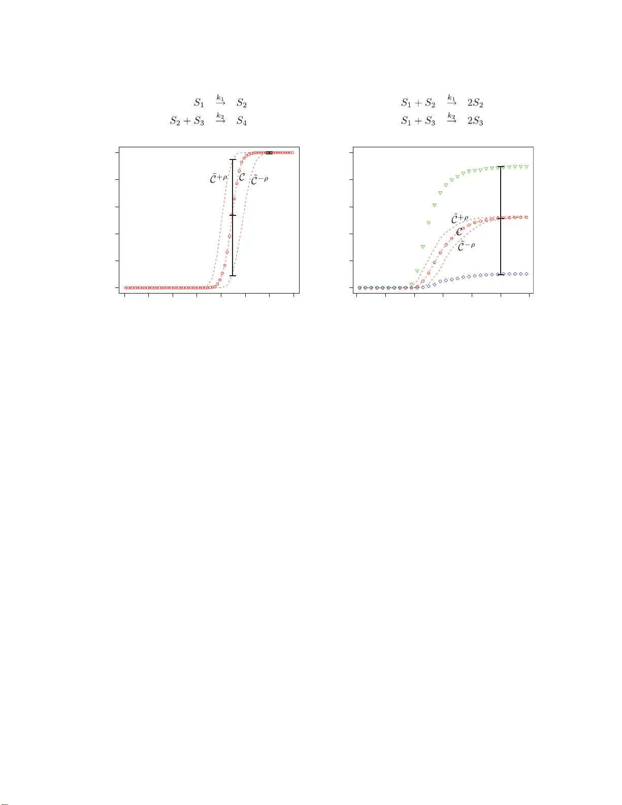
Robust Sto c hastic Chemical Reaction Net w orks and Bounded T au-Leaping Da vid Solo veic hik ∗ dsolov@calt ech.edu Abstract The behavior o f so m e sto c hastic chemical reaction netw or ks is largely unaﬀected by slight inaccur acies in reactio n r ates. W e formalize the robustness o f state probabilities to reaction rate deviations, and describe a formal connection b etw een robustness and eﬃciency of simulation. Without robustness guar antees, sto chastic simulation seems to require computational time pro po rtional to t he total num b er of reaction event s. Even if the co ncentration (molecular count per v olume) stays b ounded, the n umber of reac- tion events can b e linea r in the duration o f simulated time and total molecula r count. W e show that the b ehavior o f robust s ystems can b e predicted s uch that the compu- tational work scales linearly with the duratio n of simulated time and concentration, and o nly po lylogar ithmically in the total molecular count. Th us our asymptotic anal- ysis captur e s the dramatic sp eedup when molecula r c ounts a re large , and shows that for b ounded c oncentrations the computation time is essentially in v aria n t with molecu- lar count. Finally , by noticing that e ven r obust sto chastic chemical reaction netw orks are ca pable of embedding complex computationa l problems, we ar gue that the linear depe ndence o n sim ulated time a nd co ncent r ation is likely optimal. 1 In tro d uction The sto chastic c hemical reaction net work (SCRN) m o del of c hemical kinetics is used in c hemistry , physic s , a n d computational biology . It describ es inte r actions inv olving inte - ger n u m b er of molecules as Mark o v ju mp pro cesses (McQuarrie, 1967; van Kamp en, 1997; ´ Erdi & T´ oth, 1989; Gillespie, 1992), and is used in domains wh ere the traditional mo del of deterministic con tinuous mass a ction kinetics is in v alid due to small mol ecular counts. Small molecular coun ts are pr ev alen t in biology: for example, o ve r 80% of the genes in the E. c oli c hromosome are expressed at f ew er than a hundred copies p er cell, with some k ey con trol factors present in quan tities under a d ozen (Guptasarma, 1995; Levin, 1999). Indeed, exp er- imen tal observ ations and computer sim ulations ha ve conﬁrmed that stoc hastic eﬀects can b e physio logically signiﬁcan t (McAdams & Arkin , 1997; Elo w itz et al., 2002; Suel et al., 2006). Consequent ly , the sto chastic mo del is w idely emp lo y ed for m o deling cellular pro cesses (e.g., Arkin et al. (1998)) and is included in numerous soft ware pac k ages (V asudev a & Bhalla , ∗ Department of CNS , California Institute of T echnology , Mail Co de 136-93, Pasa d ena, CA 91125-9300, USA. V oice: (626) 395-5707, F ax: (626) 584-0630 1 2004; K ierzek, 2002 ; Adalsteinsson et al., 2004). ∗ The stochastic mo del b ecomes equ iv alen t to the classica l la w of mass actio n when the molecular counts of all participati n g sp ecies are large (Ku rtz, 1972; Ethier & Kurtz, 1986). Gillespie’s sto chastic simulat ion algorithm (SSA) can b e used to mo del the b ehavio r of S C RNs (Gillespie, 1977). Ho we ver, simulati on of systems of inte r est often requ ires an unfeasible amount of computatio nal time. Some work has fo cused on optimizing sim ulation of large S CRNs — many diﬀerent sp ecies and reaction c h annels. F or example, certain tr icks can impro ve the s p eed of deciding whic h reaction occurs next if there are m an y p ossible c hoices (e.g., Gibs on & Bruc k (2000)). Ho wev er, for the p urp oses of this pap er we supp ose that the num b er of sp ecies and reactions is relativ ely small, and that it is fundamenta lly the num b er of reactio n o ccurrences in a giv en in terv al of time that presen ts the diﬃculty . Because SS A simula tes ev ery single r eaction ev ent, sim u lation is slo w when the num b er of reaction ev ents is large. On the face of it, sim u lation sh ould b e p ossib le without explicitly mo deling ev ery reac- tion o ccurr ence. In th e mass action limit, fast s im ulation is ac hiev ed using numerical ODE solv ers. The complexit y of the simulatio n d o es not scale at all with the actual num b er of reaction o ccur r ences b u t with ov erall sim ulation time and the concen tr ation of the sp ecies. If the v olume gets larger w ithout a signiﬁcan t increase in concen tration, mass action O DE solv ers achiev e a p rofound diﬀerence in compu tation time compared to SSA. † Moreo v er maxim um concen tration is essen tially alwa y s b ound ed, b ecause th e mo d el is only v alid f or solutions dilute en ough to b e well mixed, and ultimately b ecause of the ﬁnite densit y of matter. Ho wev er, mass action sim u lation can only b e applied if molecular counts of al l the sp ecies are large. Eve n one sp ecies th at main tains a lo w m olecular count and in teracts with other sp ecies preve n ts the use of mass action ODE solv ers. Another reason why it seems that it should b e p ossible to simula te sto c h astic c h emical systems quickly , is that for man y systems the b eha vior of inte r est d o es not d ep end cru cially up on details of ev ents. F or example bio c hemical net works tend to b e r obust to v ariations in concen tr ations and kin etic p arameters (Morohashi et al., 2002; Alon, 2007). If these systems are robust to many kinds of p erturbations, includ ing slopp iness in s imulation, can w e tak e adv an tage of this to sp eed up sim u lation? F or example, can w e approac h the sp eed of ODEs b ut allo w molecular counts of some sp ecies to b e small? Indeed, tau-leaping algorithms (e.g ., Gillespie (2001 ); Rathin am et al. (20 03 ); Cao et al. (2006), see Gillespie (2007) for a review) are b ased on the idea that if we allo w r eaction pr op ensities to r emain constan t for some amoun t of time τ , b ut therefore deviate slightly from their correct v alues, w e d on’t hav e to explicitly sim ulate ev ery reaction that o ccurs in this p erio d of time (and can th u s “leap” by amount of time τ ). In this pap er w e formally deﬁne r obustness of the probabilit y that the sy s tem is in a certain s tate at a certain time to p ertur bations in r eaction pr op ensities. W e also pro v id e a metho d f or pro vin g that certain simple systems are robu s t. W e then d escrib e a n ew appro x- ∗ Some stochastic simulation implemen tations on the web: Systems Biology W ork- b ench: http://sbw .sourceforge.net ; BioSpice: http://biospice.l bl.gov ; Sto cha- stirator: http://opn srcbio.molsci.org ; STOCKS: http://www .sysbio.pl/stocks ; BioNetS: http://x.a math.unc.edu:16080 /BioNetS ; SimBiology pack age for MA TLAB: http://www .mathworks.com/pro ducts/simbiology/index.html † As an illustrativ e example, a proka ryotic cell and a euk aryotic cell may h a ve similar concentrations of proteins but va stly diﬀerent volumes. 2 imate sto chastic simulatio n alg orithm called b oun ded tau-leaping (BTL), wh ic h naturally follo ws from our deﬁnition of robustness, and pr o v ably provides correct an s w ers for robust systems. In con trast to Gillespie’s and others’ v ersions of tau-leaping, in eac h step of our algorithm the leap time, rather than b eing a fu nction of the curr en t state, is a rand om v ariable. Th is algorithm n aturally av oids some pitfalls of tau-leaping: the concent r ations cannot b ecome negativ e, and th e alg orithm scales to SSA when necessary , in a wa y that there is alw ays at least one reaction p er leap. Ho wev er, in the cases when th ere are “opp os- ing reactions” (canceling or partially cancelling eac h other) other f orms of tau-leaping may b e signiﬁcan tly faster (e.g., Rathinam & El Samad (2007)). BTL seems more amenable to theoretical analysis than Gillespie’s v ersions (Gill esp ie, 2001, 2003; Cao et al., 200 6 ), and ma y thus act as a stand -in for app ro ximate sim ulation algorithms in analytic in ve s tigations. In this pap er we use the language and to ols of com- putational complexit y theory to formally stud y ho w the num b er of leaps that BTL tak es v aries with th e maxim u m molecular count m , time span of the sim u lation t , and volume V . In lin e with the basic computational complexit y paradigm, our analysis is asymptotic and worst-ca se. “Asymptotic” means that we do not ev aluate the exact n u m b er of leaps but rather lo ok at the fun ctional form of the dep endence of their num b er on m , t , and V . This is easier to deriv e and allo ws for m aking fund amen tal distinctions (e.g ., an exp onen tial function is fundament ally larger than a p olynomial function) without getting lost in the details. “W orst-case” means that we will not stud y the b ehavio r of our algorithm on any particular c hemical system but rather upp er-b ound the num b er of leaps our algorithm tak es indep end en t of the chemical system. This will allo w us to kn o w that n o matter what the system we are tryin g to sim u late, it will n ot b e w ors e than our b ound. In this computational complexit y paradigm, w e show that in d eed robus tn ess helps. W e pro ve an up p er b ound on the num b er of steps our algorithm tak es that is loga rithmic in m , and linear in t and total concen tration C = m/V . This can b e contrasted with th e exact SSA algorithm w h ic h, in the worst case, tak es a num b er of steps that is linear in m , t , and C . S ince a logarithmic dep endence is m u ch smaller than a linear one, BTL is prov ably “closer” to the sp eed of ODE solv ers for mass act ion systems whic h hav e no dep endence on m . ∗ Finally we ask whether it is p ossible to impro ve up on BTL for robu st systems, or did w e exhaust the sp eed gains that can b e obtained due to robu stness? In the last secti on of the p ap er w e connect th is qu estion to a conjecture in computer science that is b eliev ed to b e true. With this conjecture we pro ve that th ere are r obust systems whose b eha vior cannot b e predicted in few er computational steps than the n umb er of leaps that BTL make s , ignoring m u ltiplicativ e constan t factors and p o wers of log m . W e b eliev e other v ersions of tau-leaping ha v e similar w orst-case complexities as our alg orithm , b u t pro ving equiv alen t results for them remains op en. ∗ Indeed, th e total molecular count m can b e ex tremely large compared t o its logarithm — e.g., Avo- gadro’s num b er = 6 × 10 23 while its log 2 is only 79. 3 2 Mo d el and Deﬁnitions A Sto chastic Chemic al R e action N e twork (SCRN) S sp eciﬁes a s et of N sp e cies S i ( i ∈ { 1 , . . . , N } ) and M r e actions R j ( j ∈ { 1 , . . . , M } ). The state of S is a ve ctor ~ x ∈ N N indicating the in tegral molecular coun ts of the sp ecies. ∗ A r eaction R j sp eciﬁes a reactan ts’ stoic hiometry vecto r ~ r j ∈ N N , a p ro ducts’ stoic h iometry v ector ~ p j ∈ N N , and a r eal-v alued rate constan t k j > 0. W e describ e reaction stoic hiometry using a standard c hemical “arro w” notation; for example, if there are three sp ecies, the reaction R j : S 1 + S 2 → S 1 + 2 S 3 has reactan ts v ector ~ r j = ( − 1 , − 1 , 0) and pro d ucts ve ctor ~ p j = (1 , 0 , 2). A reaction R j is p ossible in state ~ x if there are enough react ant molecules: ( ∀ i ) x i − r ij ≥ 0. Then if react ion R j o ccurs (or “ﬁres”) in state ~ x , the state c h anges to ~ x + ~ ν j , where ~ ν j ∈ Z N is th e state c hange v ector for reaction R j deﬁned as ~ ν j = ~ p j − ~ r j . W e follo w Gillespie and others and allo w unary ( S i → . . . ) and bimolecular (2 S i → . . . or S i + S i ′ → . . . , i 6 = i ′ ) r eactions only . Sometimes the m o del is extended to higher-order reactions (van Kamp en, 1997), but the merit of th is is a matter of some contro v ersy . Let us ﬁx an S CRN S . Give n a starting state ~ x 0 and a ﬁxed vo lu me V , w e can deﬁn e a con tinuous-time Marko v p ro cess w e call an SSA pr o c ess † C of S according to the f ollo wing sto c hastic kinetics. Giv en a current state ~ x , the prop ensit y function a j of r eaction R j is deﬁn ed so that a j ( ~ x ) dt is the probability that one R j reaction will o ccur in th e next inﬁnitesimal time in terv al [ t, t + dt ). If R j is a unimolecular r eaction S i → . . . then the prop ens it y is p rop ortional to th e num b er of molecules of S i currentl y present s ince eac h is equally likely to react in the next time instant ; sp eciﬁcally , a j ( ~ x ) = k j x i for reaction rate constan t k j . If R j is a bimolecular reaction S i + S i ′ → . . . , where i 6 = i ′ , then the r eactio n prop ens it y is p rop ortional to x i x i ′ , whic h is the num b er of wa ys of choosing a m olecule of S i and a molecule of S i ′ , since eac h p air is equally like ly to react in the next time instant . F urther, the probability that a particular pair reacts in the next time ins tant is inv ersely prop ortional to the v olum e, resulting in the prop en sit y function a j ( ~ x ) = k j x i x i ′ V . If R j is a bimolecular reaction 2 S i → . . . then the num b er of wa ys of choosing t wo molecules of S i to react is x i ( x i − 1) 2 , and the prop en s it y function is a j ( ~ x ) = k j x i ( x i − 1) 2 V . Since the pr op ensit y function a j of reaction R j is d eﬁ ned so that a j ( ~ x ) dt is the pr ob a- bilit y that one R j reaction will o ccur in the n ext inﬁnitesimal time interv al [ t, t + dt ), state transitions in the SSA pro cess are equiv alen tly d escrib ed as follo ws: If the sys tem is in state ~ x , no further reactio n s are p ossible if P a j ( ~ x ) = 0. Otherwise, the time un til the next reaction o ccurs is an exp onenti al rand om v ariable with r ate P j α j ( ~ x ). The probabilit y that next reaction will b e a particular R j ∗ is α j ∗ ( ~ x ) / P j α j ( ~ x ). W e are in terested in p redicting the b ehavi or of SSA pr o cesses. While there are p oten- tially man y diﬀeren t questions that we could b e tr y in g to answer, for sim p licit y we deﬁne the pr e diction pr oblem as follo ws. Giv en an SS A p ro cess C , a time t , a state ~ x , and δ ≥ 0, predict ‡ whether C is in ~ x at time t , suc h that the probabilit y that th e prediction is incor- ∗ N = { 0 , 1 , 2 , . . . } and Z = { . . . , − 1 , 0 , 1 , . . . } . † It is exactly the sto c hastic pro cess simula ted by Gilles p ie’s St ochastic Sim u lation Algorithm (SSA) (Gillespie, 1977). ‡ W e phrase th e prediction problem in terms appropriate for a sim ulation algori thm. An alternative form ulation would b e the problem of estimating the probability that the SSA process is in ~ x at time t . T o b e able to solve this problem using a simulation algorithm w e can at most require that with probabilit y at least δ 1 the estimate is within δ 2 of the tru e p robabilit y for some constants δ 1 , δ 2 > 0. This can b e attained 4 rect is at most δ . In other w ord s w e are in terested in algorithmically generating v alues of a Bernoulli rand om v ariable I ( ~ x, t ) suc h that the p robabilit y that I ( ~ x, t ) = 1 w hen C is not in ~ x at time t plu s the probabilit y that I ( ~ x, t ) = 0 when C is in ~ x at time t is at most δ . W e assume δ is some small p ositiv e constan t. W e can easily extend th e pr ediction problem to a set of states Γ rather than a s ingle target state ~ x by asking to p redict whether the pro cess is in any of the states in Γ at time t . Since Γ is mean t to captur e some qualitativ e feature of the S SA pro cess that is of interest to us, it is called an outc ome . By decreasing the v olume V (wh ic h sp eeds u p all bim olecular r eactions), increasing t , or allo wing for more molecules (up to some b oun d m ) we are increasing the num b er of reaction o ccurrences that w e ma y n eed to consider. Thus for a ﬁxed SC RN, one can try to u pp er b ound the computational complexit y of the pred iction prob lem as a fun ction of V , t , and m . Giv en a molecular count b ound m , w e deﬁne the b ounde d-c ount pr e diction pr oblem as b efore, but allo wing an arbitrary answ er if the molecular count exceeds m within time t . Su pp ose P is a b ound ed-coun t prediction pr ob lem with molecular count b ound m , error b ound δ , ab out time t and an SSA pro cess in which the v olume is V . W e then say P is a ( m, t, C , δ ) - pr e diction pr oblem where C = m/V is a b ound on the maxim um concentrat ion. ∗ Fixing some small δ , w e stud y ho w the compu tational complexity of solving ( m, t, C , δ )-prediction problems ma y scale w ith in creasing m , t , and C . If th e ( m, t, C, δ )-prediction problem is regarding an outcome Γ consisting of multi ple states, w e require the problem of deciding whether a particular state is in Γ to b e easily solv able. Sp eciﬁcally w e requir e it to b e solv able in time at most p olylogarithmic in m , w h ic h is true for an y natural pr oblem. It has b een observ ed that p erm itting p rop ensities to deviate sligh tly from their correct v alues, allo ws for muc h faster s im ulation, esp ecially if the molecular counts of some sp ecies are large. Th is idea forms the basis of app ro ximate sto c hastic sim ulation algorithms suc h as tau-leaping (Gillespie, 2001). As opp osed to th e exact SSA p ro cess d escrib ed ab o v e, consider letting th e pr op ensity function v ary sto c h astically . Sp eciﬁcally , w e deﬁne new prop ens it y fu nctions a ′ j ( ~ x, t ) = ξ j ( t ) a j ( ~ x ) where { ξ j ( t ) } are random v ariables indexed by reaction and time. The v alue of ξ j ( t ) describ es the d eviation from the correct pr op ensit y of reaction R j at time t , and shou ld b e close to 1. F or any SS A pro cess P we can deﬁn e a new sto c hastic pr o cess called a p e rturb ation of P thr ou gh the c h oice of the distributions of { ξ j ( t ) } . Note th at the n ew pro cess may not b e Mark o v, and ma y n ot p ossess Po iss on transition probabilities. If there is a 0 < ρ < 1 such that ∀ j, t , (1 − ρ ) ≤ ξ j ( t ) ≤ (1 + ρ ), then we call th e new pr o cess a ρ -p erturb ation . There may b e systems exhibiting b eha vior suc h that any sligh t inexactness in the calculation of p rop ensities quickly gets ampliﬁed and results in qualitativ ely diﬀeren t b eha vior. Ho w eve r , for some pro cesses, if ρ is a small constan t, th e ρ -p erturbation may b e a go o d approximat ion of the SSA p ro cess. Th at a ρ - p ertur b ation is b ound ed multiplic ative ly (i.e., that ξ j ( t ) acts multiplicativ ely) corresp onds to our intuiti ve notion that prop ortionally larger d eviations are required to h a v e an eﬀect if the aﬀected prop ensit y is large. W e no w deﬁne our notion of robustness. Intuitiv ely , we wan t the prediction problem to not b e aﬀected ev en if r eaction pr op ensities v ary sligh tly . F ormally , w e sa y an SS A pro cess C i s ( ρ, δ ) -r obust w ith resp ect to state ~ x at time t if for any ρ -deviating pro cess ˜ C based by runn ing th e simulation algorithm a constan t number of times. ∗ Maxim u m concentrati on C is a more natural measure of complexity compared to V b ecause similar to m and t , comput ational complexit y increases as C increases. 5 on C , th e probabilit y of b eing in ~ x at time t is w ithin plus or minus δ of the corresp ond ing probabilit y for C . This deﬁnition can b e extended to an outcome Γ similar to the deﬁn ition on th e pred iction problem. Finally w e sa y an SSA pro cess C is ( ρ, δ ) - r obust with r e sp e ct to a pr e diction pr oblem (or b oun ded-count prediction problem) P if C is ( ρ, δ )-robust with resp ect to the same state (or outcome) as sp eciﬁed in P , at the same time t as sp eciﬁed in P . F or simplicit y , we often use asymptotic notation. Th e notation O (1) is us ed to denote an unsp eciﬁed p ositiv e constan t. This constant is p oten tially diﬀerent ev ery time the expression O (1) app ears. 3 Robustness Examples In this section w e elucidate our notion of robustness by considering some examples. In gen- eral, th e question of whether a give n SSA p ro cess is ( ρ, δ )-robust for a p articular outcome seems a diﬃ cu lt one. The problem is esp ecially hard b ecause w e ha ve to consider eve r y p ossible ρ -p erturbation — th us we may not ev en b e able to giv e an appro x im ate charact er- ization of r obustness by sim ulation w ith SSA. Ho wev er, we can c haracterize the robu stness of certain (simple) systems. F or an SSA pro cess or ρ -p ertur b ation C , and outcome Γ, let F Γ ( C , t ) b e the probabilit y of b eing in Γ at time t . Consider the SCRN sh o wn in Figure 1(a). W e start with 300 molecules of S 1 and S 3 eac h, and are inte r ested in the outcome Γ of having at lea st 150 molecules of S 4 . The dashed line with circles sho ws F for the correct SSA pro cess C . (All plots of F are estimated fr om 10 3 SSA runs.) T he tw o dashed lines without circles sho w F for tw o “extremal” ρ -p ertur bations: ˜ C + ρ with constan t ξ j ( t ) = 1 + ρ , and ˜ C − ρ with constan t ξ j ( t ) = 1 − ρ . What can w e sa y ab out other ρ -p erturb ations, particularly where the ξ j ( t ) hav e muc h more complicat ed d istributions? I t turns out that for this SCRN and Γ, w e can p ro ve that any ρ -p erturbation f alls within the b ounds set b y the t wo extremal ρ -p erturbations ˜ C − ρ and ˜ C + ρ . Thus F for an y ρ -p ertu rbation falls within the dashed lines. F o r mally , C is monotonic with resp ect to Γ u sing th e d eﬁnition of m onotonicit y in Ap p endix A.3. This is easily prov en b y Lemma A.5 b ecause ev ery sp ecies is a reactan t in at most one reaction. Then by Lemma A.4, F Γ ( ˜ C − ρ , t ) ≤ F Γ ( ˜ C , t ) ≤ F Γ ( ˜ C + ρ , t ) for any ρ -p erturb ation ˜ C . T o s ee how the robustness of this system can b e quan tiﬁed using our deﬁnition of ( ρ, δ )- robustness, ﬁrst consid er t wo time p oin ts t = 4 . 5 and t = 6. A t t = 4 . 5, the pr obabilit y that the correct SSA pro cess C has pr o duced at least 150 m olecules of S 4 is sligh tly more than 0 . 5. The corresp ond ing probability for ρ -p ertu rbations of C can b e no larger than about 0 . 95 and no s maller than ab out 0 . 1. Thus C is ( ρ, δ )-robust with resp ect to outcome Γ at time t = 4 . 5 for ρ = 0 . 1 and δ app ro ximately 0 . 45, bu t not for smaller δ . On th e other hand at t = 6, the dashed lines are essentiall y on top of eac h other, resulting in a tiny δ . In f act δ is sm all for all times less than ap p ro ximately 3 . 5 or greater th an app ro ximately 5 . 5. What in formation did we need to b e able to measure ( ρ, δ )-robustness? Pro cesses ˜ C − ρ and ˜ C + ρ are simp ly C scaled in time. Thus kno win g ho w F Γ ( C , t ) v aries with t allo ws one to quan tify ( ρ, δ )-robu stness at the v arious times; F Γ ( C , t ) can b e estimated from m u ltiple S SA runs of C as in Figure 1. Intuiti v ely , C is ( ρ, δ )-robus t for small δ at all times t when F Γ ( C , t ) do es not c h an ge quickly with t (see App endix A.3). F or systems that are not monotonic, 6 0.0 0.5 1.0 1.5 2.0 2.5 3.0 0.0 0.2 0.4 0.6 0.8 1.0 Time Probability of at least 160 molecules of S 2 0 1 2 3 4 5 6 7 0.0 0.2 0.4 0.6 0.8 1.0 Time Probability of at least 150 molecules of S 4 b) a) Figure 1 : Examples of SCRNs exhibiting co ntrasting degrees of robustness. The SSA pro ce ss C and o utcome Γ a re deﬁned for the tw o sys tems by: (a) Rate constants: k 1 = 1, k 2 = 0 . 001; sta r t state: ~ x 0 = (300 , 0 , 300 , 0 ); outcome Γ: x 4 ≥ 1 50. (b) Rate co ns tants: k 1 = 0 . 01, k 2 = 0 . 01; start state: ~ x 0 = (3 00 , 10 , 10); outcome Γ: x 2 ≥ 1 60. Plots show F Γ ( · , t ) for a n SSA pro ces s or ρ -p erturbation estimated from 10 3 SSA runs. (Dashed line with circles) O riginal SSA pro cess C . (Dashed lines witho ut circ le s) The tw o extremal ρ -p erturbatio ns: ˜ C + ρ with cons tant ξ j ( t ) = 1 + ρ , and ˜ C − ρ with constant ξ j ( t ) = 1 − ρ . F or SCRN (b) w e als o plot F Γ ( · , t ) for a ρ -p erturbation with constant ξ 1 ( t ) = 1 + ρ , ξ 2 ( t ) = 1 − ρ (triangles), o r constant ξ 1 ( t ) = 1 − ρ , ξ 2 ( t ) = 1 + ρ (diamonds). Perturbation para meter ρ = 0 . 1 thr o ughout. kno win g ho w F Γ ( C , t ) v aries with time ma y not h elp with ev aluating ( ρ, δ )-robustness. Indeed, for a con trasting example, consider the SCRN in Figure 1(b ). W e start with 300 molecules of S 1 , 10 molecules of S 2 , and 10 molecules of S 3 , and we are in terested in the outcome of ha ving at least 160 molecules of S 2 . Since S 1 is a reacta nt in b oth reactions, Lemma A.5 cannot b e used. In fact , the ﬁgure sho w s t wo ρ -p ertur bations (triangles and diamonds) that clearly escap e fr om the b oundaries set by the dashed lines. T he triangles sho w F for the ρ -p erturbation where the ﬁ rst reaction is maximally s p ed up and the second reaction is maximally slo wed d o wn. (Vice versa for the d iamonds.) F or charact er ization of the r ob u stness of this sys tem via ( ρ, δ )-robustness, consider th e time p oin t t = 2 . 5. T h e probabilit y of having at least 160 molecules of S 2 in the correct SS A pro cess C is around 0 . 5. Ho we ver, this probabilit y for ρ -p erturb ations of C can deviate by at least appr o ximately 0 . 4 up ward and do wnw ard as seen b y the tw o ρ -p erturbations (triangle s and diamonds). Th us at this time the system is not ( ρ, δ )-robust for δ appr o ximately 0 . 4. What ab out other ρ -deviations? It turns out that for this particular system, the t wo ρ -per tu rbations corresp ondin g to the triangles an d diamonds b ound F in the same wa y that ˜ C − ρ and ˜ C + ρ b ound ed F in th e ﬁ rst example (exercise left to the reader). Nonetheless, for general systems that are not monotonic it is not clear ho w one can ﬁnd s uc h b oun ding ρ -p erturb ation and in f act they lik ely w ould n ot exist. 7 Of course, there are other typ es of S SA p ro cess that are not lik e either of the ab o ve examples: e.g., systems that are robust at man y times bu t not monotonic. General wa ys of ev aluating robustn ess of such systems remains an imp ortant op en pr oblem. Finally , it is imp ortant to note that qu an tifying th e robu stness of SS A p r o cesses, ev en monotonic on es, seems to requir e computing many S SA ru ns. This is self-defeating when in practice one w an ts to show that the giv en SSA pro cess is ( ρ, δ )-robust in ord er to justify th e use of an appr oximate simulatio n algorithm to quic kly sim u late it. In these cases, we ha ve to consider ( ρ, δ )-robu stness a theoretical notion only . Note, ho wev er, that it ma y b e m u c h easier to s ho w that a system is not r obust by comparing the sim ulation ru ns of diﬀerent ρ -p erturb ations, since the r uns can b e qu ickly obtained using fast app ro ximate simulati on algorithms suc h as that present ed in th e next section. 4 Bounded T au-L eaping 4.1 The Algorithm W e argued in th e Introd uction that sloppiness can allo w for faster simulat ion. In th is section w e giv e a new appro xim ate sto chastic sim ulation algorithm called b ounde d tau- le aping (BTL) th at simulate s exactly a certain ρ -p erturbation rather than the original SSA pro cess. Consequently , the algorithm solve s the prediction pr oblem with allo wed error δ for ( ρ, δ )-robust SSA pro cesses. The algorithm is a v arian t of existing tau-leaping algorithms (Gillespie, 2007). How ev er, while other tau-lea ping algorithms hav e an implicit notion of robustness, BTL is formally compatible with our explicit deﬁnition. As we’l l see b elo w, our algorithm also has certain other adv anta ges o v er many p revious tau-leaping implemen tations: it naturally disallo ws negativ e concen trations and scales to SS A in a manner that there is alwa ys at least one reaction p er leap. It also seems easier to analyze formally; obtaining a result similar to Theorem 4.1 is an op en question for other tau-leaping v arian ts. BTL h as o ve r all form t ypical of tau-leaping algorithms. Rather than sim u lating every reaction o ccur r ence explicitly as p er the S SA, BTL d ivides th e sim u lation into leaps wh ic h group m u ltiple reaction eve nts. T he p rop ensities of all of the reactio n s are assumed to b e ﬁxed throughout the leap. This is ob viously an approxi mation since eac h reaction ev ent af- fects molecular count s and therefore the prop en s ities. How ev er, this app ro ximation is useful b ecause sim u lating the system with the assump tion that prop ensities are ﬁxed turns out to b e m u c h easier. Ins tead of ha vin g to draw rand om v ariables for eac h reactio n o ccurrence, the num b er of r andom v ariables dra wn to determine h o w m an y reaction ﬁrings o ccurr ed in a leap is in dep end en t of the num b er of reaction ﬁ rings. Thus we eﬀectiv ely “leap” o ver all of th e reactions within a leap in few computational steps. If molecular counts do not c hange b y m u c h within a leap then the ﬁxed pr op ensities are close to th eir correct SS A v alues and the approxima tion is go o d . Our deﬁ n ition of a ρ -p erturbation allo ws us to formally deﬁne “go o d”. W e w ant to guar- an tee th at th e appro x im ate pr o cess that tau-leaping actually simulates is a ρ -p erturb ation of the exac t SSA p r o cess. W e can ac hiev e this as follo ws. If ~ x is the state on whic h the leap started, th roughout the leap the sim u lated reaction p rop ensities are ﬁxed at their SSA p rop ensities on ~ x : a j ( ~ x ). Then for an y state ~ y within the leap we wan t the cor- 8 rect SSA pr op ensities a j ( ~ y ) to s atisfy the follo w in g ρ -p erturb ation c onstr aint (0 < ρ < 1): (1 − ρ ) a j ( ~ y ) ≤ a j ( ~ x ) ≤ (1 + ρ ) a j ( ~ y ). As so on as w e reac h a state ~ y for which this constrain t is violated, we start a n ew leap at ~ y which will use simulate d reaction p rop ensities ﬁx ed at a j ( ~ y ). This ensures that at an y time in the simulat ion, there is some (1 − ρ ) ≤ ξ j ( t ) ≤ (1 + ρ ) suc h that multiplying the correct SSA prop ensit y of reaction R j b y ξ j ( t ) yields the p rop en- sit y of R j that the sim ulation algorithm is actually us in g. Therefore, we actually simulate a ρ -p erturb ation, and for ( ρ, δ )-robu st SSA pro cesses, the algorithm can b e used to pro v ably solv e the p r ediction problem with error δ . Can w e implement this sim ulation quickly , and, as promised, do little computation p er leap? Note that in order to limit the maxim um prop ensit y deviation in a leap, w e n eed to mak e the leap dur ation b e a rand om v ariable dep endent up on the sto c h astic ev ents in th e leap. If we ev aluate a j ( ~ y ) after eac h reaction o ccurrence in a leap to verify the satisfaction of the ρ -p erturbation constraint, w e do n ot sa v e time o ver S SA. How ev er, w e can a v oid this b y u sing a stricter constraint we call the { ε ij } -p erturb ation c onstr aint (0 < ε ij < 1), deﬁn ed as follo ws. If the leap starts in state ~ x , reaction R j is allo wed to change the molecular count of sp ecies S i b y at most plus or m in u s ε ij x i within a leap. Again, as so on as we r eac h a state ~ y where this constraint is v iolated, we start a new leap at ~ y . ∗ F or an y ρ , we can ﬁn d a set of { ε ij } b oun d s suc h that satisfying the { ε ij } -p erturbation constrain t satisﬁes the ρ -p erturbation constrain t. I n App en d ix A.1 we sho w that for an y SCRN, the ρ -p ertur bation constrain t is satisﬁed if ε ij ≤ 3 4 M (1 − q 1+ ρ/ 9 1+ ρ ), wher e M is the n u m b er of r eactions in the S CRN. Sim u lating a leap such that it satisﬁes the { ε ij } -p erturbation constrain t is easy an d only requires dra wing M gamma and M − 1 bin omial r andom v ariables. Supp ose the leap starts in state ~ x . F or eac h reaction R j , let b j b e the n um b er of times R j needs to ﬁr e to cause a violation of the { ε ij } b ounds for some sp ecies. Th us b j is the smallest p ositiv e in teger suc h that | b j ν ij | > ε ij x i for some S i . T o determine τ , the du ration of the leap, we do the follo wing. First w e determine wh en eac h reaction R j w ould o ccur b j times, by drawing from a gamma distribu tion with shap e parameter b j and rate parameter a j . This generates a time τ j for eac h r eaction. The leap ends as so on as some reaction R j o ccurs b j times; thus to determine the duration of the leap τ w e take the minim u m of the τ j ’s. A t this p oin t we kno w that the ﬁr st-violating reaction R j ∗ — the one with the minimum τ j ∗ — o ccurred b j ∗ times. But w e also need to kn o w h o w many times the other reactions o ccur. Consider any other reaction R j ( j 6 = j ∗ ). Give n th at th e b j th o ccurrence of reaction R j w ould h av e happ en ed at time τ j had the leap not end ed, we need to d istr ibute the other b j − 1 o ccur rences to determine how m an y h app en b efore time τ . The num b er of o ccurrences at time τ is given b y the binomial distr ibution with num b er of trials b j ( ~ x ) − 1 and success prob ab ility τ / τ j . This enables us to deﬁne BTL as s h o wn in Figure 2 . The algorithm is called “b ounded” tau-leaping b ecause the deviations of reaction p rop en- sities within a leap are alw a ys b ound ed according to ρ . Th is is in con trast with other tau-leaping algorithms, s uc h as Gillespie’s (Cao et al., 2006), in whic h th e d eviations in reaction prop ensities are sm all with high probabilit y , but not alw ays, and in fact can get ∗ An added b en eﬁt of providing { ε ij } b ounds rather than ρ as a parameter to the BTL algorithm is that it allo ws ﬂex ibilit y on the part of the user to assign less resp onsibilit y for a violation to a reaction that is exp ected to be fast compared t o a reaction that is exp ected to b e slo w. This may p otentia lly speed up the sim u lation, while still preserving th e ρ -p ertu rbation constraint. 9 0. Initialize with time t = t 0 and the sy s tem’s state ~ x = ~ x 0 . 1. With the system in state ~ x at time t , ev aluate all the prop ensities a j , and determine ﬁring b oun ds b j for all p ossib le reactions, wh ere b j is the smallest p ositiv e intege r suc h that | b j ν ij | > ε ij x i for s ome S i . 2. Generate violating times τ j ∼ Gamma( b j , a j ) for all p ossible reactions. 3. Find the ﬁrs t-violati n g reaction an d set the step size to the time of the ﬁr s t viola- tion: let j ∗ = argmin j { τ j } and τ = τ j ∗ . 4. Determine the num b er of times eac h p ossible reaction o ccurred in interv al τ : for j 6 = j ∗ , n j ∼ Binomial( b j − 1 , τ /τ j ); for j ∗ , n j ∗ = b j ∗ . 5. Eﬀect the leap by replacing t ← t + τ and ~ x ← ~ x + P j ~ ν j n j . 6. Record ( ~ x, t ) as desired . Return to Step 1, or else en d the simulation. Figure 2 : The b ounded tau-leaping (BTL) algor ithm. The algorithm is given the SCRN, the initial state ~ x 0 , the volume V , and a set of pe r turbation b ounds { ε ij } > 0 . If the state a t a sp eciﬁc time t f is des ired, the alg orithm chec k s if t + τ > t f in step (3), and if so uses τ = t f − τ , and treats all reactions as not ﬁrst- violating in step (4). Gamma( n, λ ) is a gamma distribution with shape parameter n and rate pa rameter λ . Binomial( n, p ) is a binomia l distribution with num b e r of tr ials n and success pr obability p . arbitrarily h igh if the simulation is long enough. This allo ws BTL to s atisfy our deﬁn ition of a ρ -p ertur bation, and p ermits easier analysis of the b eha vior of the algorithm (see next section). As any algorithm exactly sim ulating a ρ -p ertur bation w ould, BTL n aturally av oids negativ e concen trations. Negativ e counts can o ccur only if an imp ossible reaction happ ens — in some state ~ x reaction R j ﬁres for whic h a j ( ~ x ) = 0. But since in a ρ -p erturbation prop ens it y deviations are m u ltiplicativ e, in state ~ x , a ′ j ( ~ x, t ) = ξ j ( t ) a j ( ~ x ) = 0 and so R j cannot o ccur. F urther, no matter how small the { ε ij } b ound s are, there is alw a ys at least one reaction p er leap and th u s BTL cannot tak e more s teps than S SA. On the negativ e side, in certain cases the BTL algorithm can tak e many more leaps than Gillespie’s tau-lea p ing (Gillespie, 2001, 2003; Cao et al., 2006 ) and other ve r sions. Consider the case w here there are tw o fast r eactions that partially und o eac h others’ eﬀect (for example the reactions ma y b e reverses of eac h other). While b oth reactio n s ma y b e o ccurring very rapidly , their prop ensities ma y b e ve ry similar (e.g., Rathin am & El S amad (2007)). Gillespie’s tau-leaping will attempt to leap to a p oin t w here the molecular coun ts ha ve c h an ged enough according to the aver age d b eha vior of these reactions. How ev er, our algorithm considers eac h reaction separately and leaps to the p oint where the ﬁ rst reaction violates the b ound on the change in a sp ecies in the absence of the other reactions. T h u s in this situation our algorithm w ould p erform un necessarily many leaps for the desired lev el of accuracy . 10 4.2 Upp er Bound on the Num b er of Leaps Supp ose w e ﬁ x some SCRN of in terest, and run BTL on diﬀeren t initial s tates, v olumes, and lengths of sim ulated time. Ho w do es v arying th ese parameters c han ge th e n u m b er of leaps tak en by BTL? In this section, we pro v e that n o matter what the SCRN is, we can upp er b ound th e num b er of leaps as a fun ction of the total sim u lated time t , the vo lu me V , and the maximum total molecular coun t m encountered d u ring the sim ulation. F or simplicit y w e assume that all the ε ij are equal to some global ε . (Alt ernativ ely , the theorem and pro of can b e easily c hanged to use min/max { ε ij } v alues where appr opriate.) Theorem 4.1. F or any SCRN S with M sp e cies, any ε such that 0 < ε < 1 / (12 M ) , and any δ > 0 , ther e ar e c onstants c 1 , c 2 , c 3 > 0 such that for any b ounds on time t and total mole cular c ount m , for any volume V and any starting state, after c 1 log m + c 2 t ( C + c 3 ) le aps wher e C = m/V , either the b ound on time or the b ound on total mole cular c ount wil l b e exc e e de d with pr ob ability at le ast 1 − δ . Pr o of. The pro of is pr esen ted in App endix A.2. Note that the u pp er b ound on ε implies that the algorithm is exactly simulating some ρ -p erturb ation (see previous section). In tu itiv ely , a k ey idea in the pro of of the theorem is that th e prop ensity of a reaction decreasing a particular sp ecies is linear to the amoun t of that sp ecies (since the sp ecies must app ear as a r eactan t). This allo w s u s to b ound the decrease of an y sp ecies if a leap is sh ort. Actually this imp lies that a short leap probably increases the amount of some sp ecies by a lot (some sp ecies m ust cause a violation — if not by a decrease it m u st b e by an increase). This allo ws u s to argue th at if we hav e a lot of long leaps we exceed our time b ound t and if we ha ve a lot of short leaps w e exceed our b ound on total molec u lar count m . I n fact b ecause the eﬀect of leaps is m ultiplicativ e, logarithmically many sh ort leaps are enough to exceed m . It is in formativ e to compare this result with exact S S A, wh ic h in the worst case tak es O (1) m t ( C + O (1)) steps, since eac h reaction o ccurr ence corresp onds to an S SA step and the maxim u m reaction p rop ensity is k j m 2 /V or k j m . Sin ce m can b e v ery large, the sp eed impro vemen t can b e pr ofound. W e b eliev e, although it remains to b e p ro ven, that other v ersions of tau-leaping (see e.g., Gillespie (2007) for a review) achiev e the same asymptotic w orst case num b er of leaps as our algorithm. Ho w muc h computation is required p er eac h leap? Eac h leap inv olv es arithmetic op er- ations on the m olecular count s of the sp ecies, as we ll as drawing from a gamma and bino- mial distrib utions. S ince there are fast algorithms for obtaining instances of gamma and binomial random v ariables (e.g., Ahren s & Dieter (1978); Kachitvic h ya nukul & Schmeiser (1988)), we do n ot exp ect a leap of BTL to require muc h more computation than other forms of tau-leaping, and should not b e a ma j or con tributor to the total r unning time. Precise b ounds are dep en d en t on the mo del of computation. (In the next section w e s tate reasonable asymptotic b ounds on the compu tation time p er leap for a r andomized T uring mac hine imp lemen tation of BTL.) 11 5 On the Computational Complexit y of the Prediction Prob- lem for Robust SSA Pro cesses What is the computational complexit y inherent in the p rediction problem for robus t SSA pro cesses? Is sim ulation with BTL a go o d pr o cedure for solving the problem, or are there faster metho ds not inv olving sim ulation that someho w directly compute d esired end-time probabilities withou t ev aluating the en tire tra jectory? W e ha ve sho w n that the num b er of leaps that BTL tak es scales at most linearly with t and C . Ho wev er, for some s ystems there are analytic sh ortcuts to determining the probability of b eing in Γ at time t . F or instance the “exp onenti al deca y” S CRN consisting of the single reaction S 1 → S 2 is easily solv able analyticall y (Malek-Mansour & Nicolis, 1975). The calculation of the probability of b eing in any giv en state at any giv en time t (among other questions) can b e solv ed in time that gro ws minimally with t and C . In deed, it ma y seem p ossible that robust SSA pro cesses are someho w b eha viorally weak and that their b ehavio r can b e easily predicted. In order to b e able to consider these questions formally , we sp ecify our mo del of com- putation as b eing r andomized T u r ing m ac hines (see b elow). W e say that compu tation time p olylogarithmic in the maxim um tot al molecular co unt m is eﬃcient in m (in fact log m computation time is requ ir ed to simply r ead in th e initial s tate of the SSA pro cess and target state of the prediction problem). In this s ection we p ro ve that for an y algorithm eﬃcien t in m solving prediction pr oblems for robust S SA pro cesses, there are p r ediction problems ab out suc h p ro cesses that cannot b e solved faster than lin ear in t and C . W e pro ve this result assuming a r easonable conjecture in computational complexit y theory . Then, with certain ca veats r egardin g implemen ting BTL on a T uring mac h ine, sim ulation with BTL is optimal in t and C for solving prediction pr ob lems for robu st SSA pro cesses among algorithms eﬃcien t in m . W e use th e standard mo del of compu tation whic h captures sto c h astic b eha vior: ran- domized T ur ing machines (TM). A r andomized TM is a n on-deterministic TM ∗ allo wing m ultiple p ossible transitions at a p oint in a computation. The actual transition tak en is uniform o v er the c hoices. (See for example Sip s er (1997) for equiv alen t f ormalizatio n s.) W e sa y a giv en TM on a giv en input run s in computational time t tm if there is no set of random c hoices th at m akes the machine ru n longer. W e wan t to sho w that for some S CRNs, there is no method of solving the prediction problem fast, no m atter ho w cleve r we are. W e also w ant these s to c hastic p ro cesses to b e robust despite h a ving d iﬃcult p rediction problems. W e use the follo wing tw o ideas. First, a metho d b ased on Angluin et al. (2006) shows that predicting the output of give n r andom- ized TMs can b e done b y solving a pr ediction pr oblem for certain robust SS A pro cesses. Second, an op en conjecture, but one that is strongly compatible with th e basic b eliefs of computational complexit y theory , b oun d s how quic kly th e output of r andomized TMs can b e determined. Computational complexit y theory concerns measurin g ho w the computational r esources required to solv e a giv en problem s cale with input size n (in b its). T he t wo most p rev alen t eﬃciency measures are time and space — the num b er of TM steps and the length of the TM tap e required to p erform the computation. W e say a Bo olean function f ( x ) is pr ob a- ∗ Arbitrary ﬁn ite num b er of states and tap es. Without loss of generalit y , w e can ass u me a b in ary alphab et. 12 bilistic al ly c omputable by a T M M in time t ( n ) (wh ere n = | x | ) and space s ( n ) if M ( x ) ru ns in time t ( n ) using space at most s ( n ), an d with pr obabilit y at least 2 / 3 outpu ts f ( x ). ∗ A basic tenet of compu tational complexit y is that allo w ing asymptotically more computation time t ( n ) alw a ys expand s the set of problems that can b e solv ed. Thus it is widely b eliev ed that for an y (reasonable) t ( n ), there are “ t ( n )-hard” functions that can b e p robabilistically computed in t ( n ) time, but n ot in asymptotically s m aller time. † F or our argument we will need suc h a t ( n )-hard fun ction, b ut one that do es not requir e to o m uch sp ace. F ormally we assume th e follo wing hier ar chy c onje ctur e : Conjecture 5.1 ((Probabilistic, Space-Limited) Time Hierarc hy) . F or any α < 1 , and p olynomials t ( n ) and s ( n ) such that t ( n ) α and s ( n ) ar e at le ast line ar, ther e ar e Bo ole an functions that c an b e pr ob abilistic al ly c ompute d within time and sp ac e b ounds b ounds t ( n ) and s ( n ) , but not in time O (1) t ( n ) α (with unr estricte d sp ac e usage). In tu itiv ely , w e tak e a Bo olean function that requires t ( n ) time and em b ed it in a chemical system in such a w ay that solving the prediction problem is equiv alen t to p robabilistically computing the fun ction. The conjecture implies that w e cannot solv e th e pr ediction prob- lem fast enough to allo w us to solve the compu tational problem faster than t ( n ). F urther, since the resulting SSA pro cess is robu s t, the resu lt lo wer-b ounds the compu tational com- plexit y of the prediction problem f or r ob u st pro cesses. Note th at we need a time hierarch y conjecture that restricts the space usage and talks ab out p robabilistic computation b ecause it is imp ossible to em b ed a TM computation in an SCR N suc h that its computation is error free (Solo v eic h ik et al., 2008), and fur ther such embed d ing seems to require more time as the space u sage increases. The follo wing theorem lo wer-boun ds th e compu tational complexit y of the pred iction problem. The b oun d holds ev en if we restrict ourselve s to r obust pr o cesses. It shows that this computatio nal complexit y is at least linear in t and C , as long as the dep endence on m is at most p olylogarithmic. It lea ve s the p ossib ilit y that ther e are algorithms for solving th e prediction problem that require computation time more than p olylogarithmic in m but less than linear in t or C . Let the prediction problem b e sp eciﬁed by giving the SS A pro cess (via the initial state and v olume), the target time t , and th e target outcome Γ in some standard enco ding suc h th at w hether a state b elongs to Γ can b e computed in time p olylogarithmic in m . Theorem 5.1. Fix any p erturb ation b ound ρ > 0 and δ > 0 . Assuming the hier ar chy c onje ctur e (Conje ctur e 5.1), ther e is an SCRN S such that for any pr e diction algorithm A and c onstants c 1 , c 2 , β , η , γ > 0 , ther e is an SSA pr o c ess C of S and a ( m, t, C, 1 / 3) -pr e diction pr oblem P of C such that A c annot solve P i n c omputational time c 1 (log m ) β t η ( C + c 2 ) γ if η < 1 or γ < 1 . F u rther, C is ( ρ, δ ) -r obust with r esp e c t to P . Pr o of. The pro of is pr esen ted in App endix A.5. ∗ Any other constant probability b ounded a wa y from 1 / 2 will do just as wel l: t o achiev e a larger constant probabilit y of being correct, we can repeat the computation a constant num b er of times and take ma jority vote. † If we do not allo w any chance of error, th e corresp onding statement is prove n as the (deterministic) time hierarch y theorem (Sip ser, 1997). Also see Barak (2002); F ortno w & Santhanam ( 2006) for progress in proving the p rob ab ilistic v ersion. 13 In App endix A.6 , we argue that BTL on a randomized TM r u ns in total computation time O (1)((log( m )) O (1) + l ) t ( C + O (1)) where, in eac h leap, p olylogarithmic time in m is required for arithmetic manipu lation of molecular counts, and l captures the extra compu tation time requ ired for th e real n u m b er op erations and drawing from the gamma and binomial distribu tions. Here l is p oten tially a fu n ction of m , V , t , and the bits of precision u sed, but assuming eﬃcien t metho ds for dra w in g the r andom v ariables l is likel y very sm all compared to the total num b er of leaps. Then, assuming w e can ignore errors in tro d uced due to ﬁn ite precision arithmetic and appro ximate random num b er generation, sim ulation with BTL is an asymp toticall y optimal w ay in t and C of solving th e pr ediction pr oblem for robust p ro cesses among metho ds eﬃcien t in m . 6 Discussion The b ehavio r of m an y sto c h astic c h emical reaction net works d o es n ot dep end crucially on getting the reaction pr op ensities exactly righ t, p rompting our deﬁnition of ρ -p erturb ations and ( ρ, δ )-robustness. A ρ -p erturbation of an S SA pr o cess is a sto chasti c pro cess with sto c hastic deviations of the reaction p rop ensities f rom their correct SSA v alues. These deviations are multiplicat iv e and b ounded b et we en 1 − ρ and 1 + ρ . If w e are concerned with h o w lik ely it is that the SS A pr o cess is in a giv en state at a given time, then ( ρ, δ )- robustness captures how far these probabilities ma y deviate for a ρ -p erturb ation. W e f ormally sho we d that predicting the b ehavio r of robus t pro cesses do es not require sim ulation of eve r y reaction ev ent. Sp eciﬁcally , we describ ed a n ew appr oximate sim ulation algorithm calle d b ound ed tau-leaping (BTL) th at simulate s a certain ρ -p ertur bation as opp osed to the exact S SA pro cess. The accuracy of the algorithm in making pr edictions ab out the state of the s y s tem at given times is guarant eed for ( ρ, δ )-robust pro cesses. W e pro ved an upp er b ound on the n umb er of leaps of BTL that helps explain the sa vings o v er SSA. The b oun d is a f u nction of the desired length of s im ulated time t , volume V , and maxim um molecular coun t encoun tered m . This b ound scales linearly with t and C = m/V , but only logarithmically with m , while the total num b er of reactions (and th erefore SS A steps) ma y scale linearly w ith t , C , and m . When total concent ration is limited, but the total molecular count is large, th is represents a profound improv emen t o v er SSA. Because the num b er of BTL leaps scales only logarithmically with m , BTL asymptotically nears the sp eed of mass action ODE solv ers — w h ic h hav e n o dep endence on m . W e also argue that asymptotically as a function of t and C our algorithm is optimal in as far as no algorithm can ac h iev e sub linear dep en d ence of the n u m b er of leaps on t or C . Th is result is pr ov en based on a reasonable assumption in compu tational complexit y theory . Unlike Gillespie’s tau-leaping (Cao et al., 2006), our algorithm seems b etter su ited to theoretical analysis. Th us wh ile we b eliev e other versions of tau-leaping ha ve similar wo r st-case ru nning times, the results analogous to those w e ob tain for BTL r emain to b e prov ed. Our r esults can also b e seen to addr ess the follo win g question. If concerned solely with a particular outcome r ather than with the entire p ro cess tra jectory , can one alw a ys ﬁ nd certain sh ortcuts to d etermine the probabilit y of the outcome withou t p erf orming a full 14 sim ulation? Since our lo wer b ound on computation time scales lin early with t , it could b e interpreted to mean that, except in prob lem-sp eciﬁc cases, there is no shorter route to predicting the outcomes of sto chastic c h emical pro cesses than via sim ulation. Th is negativ e result h olds ev en r estricting to the class of robust SS A pro cesses. While the notion of r obustness is a u seful theoretical construct, ho w p ractical is our deﬁnition in deciding whether a giv en system is suitable to approximate simula tion via BTL or n ot? W e pr o ve that for the class of mon otonic SS A pro cesses, robustn ess is guaran teed at all times wh en in the SSA pro cess the outcome probabilit y is stable ov er an interv al of time determined by ρ . How ev er, it is n ot clear how this stability can b e determined w ithout SSA sim ulation. Even worse, few systems of int erest are monotonic. Consequen tly , it is comp elling to dev elop tec hn iques to establish r ob u stness for more general classes of systems. A r elated q u estion is w h ether it is p ossib le to connect our notion of robustness to previously studied notions in mass action stabilit y analysis (Horn & Jac k s on, 1972; Sontag, 2007). A App endix A.1 Enforcing the ρ -P erturbation Constr ain t by the { ε ij } -P ert urbation Constrain t Recall that in Section 4.1 we in tro duced t wo constraint s b ounding the n u m b er of r eaction ev ent s within a leap. If ~ x is the state at the b eginnin g of the leap, the ρ -p erturbation constrain t is satisﬁed if for every reaction R j , (1 − ρ ) a j ( ~ y ) ≤ a j ( ~ x ) ≤ (1 + ρ ) a j ( ~ y ) for any state ~ y within the leap. T he { ε ij } -p erturbation constrain t is satisﬁed if n o reaction R j c hanges the molecular coun t of sp ecies S i b y more than plu s or minus ε ij x i within the leap. F or a giv en ρ , w e wo u ld lik e to ﬁn d an app ropriate { ε ij } -p erturbation constrain t to us e in the BTL algorithm suc h that w e satisfy the ρ -p erturbation constraint, thereb y ensuring that w e are exactly simulat in g s ome ρ -p erturb ation. T o a v oid making the { ε ij } -p erturbation constrain t tighte r than n ecessary requir es kno wledge of the exact reactions in the giv en SCRN. Nev ertheless, w orst-case analysis b elo w shows that setting ε ij ≤ 3 4 M (1 − q 1+ ρ/ 9 1+ ρ ) w orks for any SC R N of M reactions. If ε ij = ε then, for any SCRN with M reactio n s, th e maxim u m c hange of an y sp ecies S i within a leap allo we d b y the { ε ij } -p erturbation constrain t is p lus or min us M εx i . W e w ant to ﬁnd an ε > 0 suc h that if the changes to all sp ecies s tay w ithin th e M ε b ound s, then no r eaction violates the ρ -p ertur bation constrain t. C onsider a bim olecular reaction R j : 2 S i → . . . ﬁrst. The algorithm sim u lates its prop ensit y as a j ( ~ x ) = k j x i ( x i − 1) /V throughout the leap. If x i = 0 or 1, then a j ( ~ x ) = 0, and as long as M ε < 1, then still a j ( ~ y ) = 0, satisfying the ρ -p erturbation constrain t for R j . Oth er w ise, if x i ≥ 2, then the SSA prop en sit y at state ~ y within th e leap is a j ( ~ y ) = k j y i ( y i − 1) / V ≤ k j (1 + M ε ) x i ((1 + M ε ) x i − 1) / V , and so the left half of the ρ -p erturb ation constrain t (1 − ρ ) a j ( ~ y ) ≤ a j ( ~ x ) is satisﬁed if (1 − ρ )(1 + M ε ) x i ((1 + M ε ) x i − 1) ≤ x i ( x i − 1). Similarly , the right half of the ρ -p ertur b ation constrain t a j ( ~ x ) ≤ (1 + ρ ) a j ( ~ y ) is satisﬁed if (1 + ρ )(1 − M ε ) x i ((1 − M ε ) x i − 1) ≥ x i ( x i − 1). These in equalities are satisﬁed for x i ≥ 2 wh en ε ≤ 3 4 M (1 − q 1+ ρ/ 9 1+ ρ ) (whic h also ensur es that M ε < 1). In a likewise manner, for a u nimolecular reaction R j : S i → . . . , th e ρ -p erturbation 15 constrain t is satisﬁed if (1 − ρ )(1 + M ε ) x i ≤ x i and (1 + ρ )(1 − M ε ) x i ≥ x i , and for a bimolecular reaction R j : S i + S i ′ → . . . , the constrain t is satisﬁed if (1 − ρ )(1 + M ε ) 2 x i x i ′ ≤ x i x i ′ and (1 + ρ )(1 − M ε ) 2 x i x i ′ ≥ x i x i ′ . It is easy to see that setting ε as ab o ve also satisﬁes the inequalities for these reaction t yp es. Throughout the pap er w e assum e that ρ , ε or { ε ij } are ﬁxed and most of our asymptotic results do n ot show dep endence on these parameters. Nonetheless, we can show that for a ﬁxed S CRN and for small enough ρ , ε can b e within the ran ge O (1) ρ ≤ ε ≤ O (1) ρ and thus scales linearly with ρ . Therefore, in asymptotic results, the dep endence on ε and ρ can b e in terchange d. Sp eciﬁcally , the ε dep end ence explored in Ap p endix A.2 can b e equally w ell expressed as a d ep enden ce on ρ . A.2 Pro of of Theorem 4.1: Upp er Bound on the Num b er of Leaps In this section w e prov e Theorem 4.1 fr om the text, w h ic h upp er-b ounds the num b er of leaps BTL tak es as a fu nction of m , t , and C : Theorem. F or any SCRN S with M sp e cies, any ε such that 0 < ε < 1 / (12 M ) , and any δ > 0 , ther e ar e c onstants c 1 , c 2 , c 3 > 0 such that for any b ounds on time t and total mole cular c ount m , for any volume V and any starting state, after c 1 log m + c 2 t ( C + c 3 ) le aps wher e C = m/V , either the b ound on time or the b ound on total mole cular c ount wil l b e exc e e de d with pr ob ability at le ast 1 − δ . W e pro ve a more detailed b ound than stated in the theorem ab o ve which explicitly shows the dep endence on ε hid den in the constant s . Also since we in tro duce the asymp totic results only the end of the argument, the intereste d reader may easily inv estigate the dep endence of the constan ts on other p arameters of the S CRN such as N , M , ν ij , and k j . W e also sho w an approac h to p robabilit y 1 that o ccurs exp onen tially fast as the b ound increases: if the b ound ab ov e ev aluates to n , then the probability that the algorithm do es not exceed m or t in n leaps is at most 2 e − O (1) n . Our argument s tarts with a co uple of lemmas. L o oking within a single leap, the ﬁrs t lemma b oun d s the d ecrease in the molecular coun t of a sp ecies due to a giv en reaction as a function of time. T he argum ent is essen tially that for a r eaction to decrease the molecular coun t of a sp ecies, th at sp ecies must b e a reactan t, and therefore the pr op ensity of the reaction is prop ortional to its molecular count. Thus we see a similarit y to an exp onen tial deca y pro cess and us e this to b ound the decrease. Note that a similar result do es not hold for the incr e ase in the molecular coun t of a sp ecies, since the molecular count of the increasing sp ecies need not b e in the prop ensit y f unction. ∗ Then the second lemma uses the u pp er b ound on how fast a sp ecies can d ecrease (the ﬁrst lemma), together with the fact that in a leap some reaction must c hange s ome sp ecies by a r elativ ely large amount, to classify leaps in to those that either (1) tak e a long time or (2) increase some sp ecies signiﬁcantly w ithout decreasing any other sp ecies by m u c h. Finally we s h o w that this implies th at if there are to o man y leaps we either violate the time b ound or the total molecular count b ound. ∗ If a reaction is con verting a popu lous sp ecies to a rare one, the rate of the increase of th e rare species can b e prop ortional to m times its molecular count. The rate of decrease, how ever, is alwa ys prop ortional to the molecular count of the decreasing sp ecies, or proportional to C times the molecular count of the decreasing sp ecies ( as w e’ll see below). 16 F or th e follo wing, v alues f and g will b e free parameters to b e d etermin ed late r . It helps to th ink of them as 0 < f ≪ g ≪ 1. Ho w long do es it tak e for a reaction to decrease x i b y g th fraction of the violation b ound εx i ? The n umb er of o ccurrences of R j to decrease x i b y g εx i or more is at least g εx i / | ν ij | . The follo win g lemma b oun ds the time requ ir ed for th ese man y o ccurr ences to happ en . Lemma A.1. T ake any f and g (0 < f , g < 1) , any r e action R j and sp e cies S i such that ν ij < 0 , any state ~ x , and any ε . Assuming that the pr op ensity of R j is ﬁxe d at a j ( ~ x ) , with pr ob ability at le ast 1 − f /g , fewer than g εx i / | ν ij | o c curr enc es of R j happ en in time f ε/ ( | ν ij | k j ) if R j is unimole cular, or time f ε/ ( | ν ij | k j C ) if R j is bimole cular. Pr o of. F or reaction R j to decrease the amoun t of S i , it m u st b e that S i is a reactan t, an d th us x i is a factor in the prop en s it y fu nction. Sup p ose R j is u nimolecular. Then a j = k j x i and the exp ected num b er of o ccur rences of R j in time f ε | ν ij | k j is a j f ε | ν ij | k j ≤ f εx i | ν ij | . The desired result then follo ws fr om Marko v’s inequalit y . I f R j is bimolecular with S i 6 = S i ′ b eing the other reactan t then a j = k j x i x i ′ V ; alternativ ely , a j = k j x i ( x i − 1) V if R j is bimolecular with iden tical reactan ts. In general for bimolecular reactio n s a j ≤ k j x i C . S o the exp ected n u m b er of o ccurr ences of R j in time f ε | ν ij | k j C is a j f ε | ν ij | k j C ≤ f εx i | ν ij | . The desired result follo ws as b efore. Let time ˜ τ b e the min im um o ver all reactions R j and S i suc h th at ν ij < 0 of 1 / ( | ν ij | k j ) if R j is unimolecular, or 1 / ( | ν ij | k j C ) if R j is bimolecular. W e can think of ˜ τ setting the units of time for our argumen t. The abov e lemma implies that with p r obabilit y at lea s t 1 − f /g no reactio n decreases x i b y g εx i or more within time f ε ˜ τ . The follo wing lemma deﬁnes t yp ical leaps; they are of tw o types: long or S i -increasing. Recall M is the n u m b er of reaction channels and N is the num b er of sp ecies. Lemma A.2. (T ypic al le aps). F or any f and g (0 < f , g < 1) , and for any ε , with pr ob ability at le ast 1 − N M f /g one of the fol lowing is true of a le ap: 1. (long le ap) τ > f ε ˜ τ 2. ( S i -incr e asing le ap) τ ≤ f ε ˜ τ , and the le ap incr e ases some sp e cies S i at le ast as x i 7→ x i + ⌈ εx i ⌉ − g M εx i , while no sp e cie s S i ′ de c r e ases as much as x i ′ 7→ x i ′ − g M εx i ′ . Pr o of. By th e un ion b oun d o ve r the M reaction c hannels and th e N sp ecies, Lemma A.1 implies th at the pr obabilit y that some reaction decreases the amount of som e sp ecies S i b y g εx i or more in time f ε ˜ τ is at most N M f /g . No w sup p ose this un luc ky ev ent do es n ot happ en . Then if the leap time is τ ≤ f ε ˜ τ , no d ecrease is enough to cause a violation of the deviation b ound s, and thus it must b e that some r eactio n R j increases some sp ecies S i b y more than εx i . (Since R j m us t o ccur an integ er num b er of times, it actually m u st increase S i b y ⌈ εx i ⌉ or more.) Since no reaction decreases S i b y g εx i or more, we can b e sur e that S i increases at least by ⌈ εx i ⌉ − g M εx i . Lemma A.3. F or any sp e cies S i , a le ap de cr e ases S i at most as x i 7→ x i − M ⌊ εx i ⌋ − 2 . Pr o of. A t most M reactions ma y b e decreasing S i . A reaction can decrease S i b y as muc h as ⌊ εx i ⌋ without causing a violation of th e deviation b ound s. T he last r eactio n ﬁr in g that causes the viola tion of the deviation b ounds ending the leap uses up at most 2 m olecules of S i (since reactions are at most bimolecular). 17 Note that a similar lemma do es not hold for Gillespie’s tau-leaping algorithms (Gillespie, 2001, 2003; C ao et al., 2006) b ecause th e num b er of reaction ﬁ r ings in a leap can b e only b ound ed probabilistically . With some small pr ob ab ility a leap can result in “catastrophic” c hanges to some molecular coun ts. Since with en ou gh time suc h ev en ts are certain to o ccur, the asymptotic analysis must consider them. Consequent ly , asymp totic results analogous to those w e der ive in this section remain to b e pr o ve d for tau-leaping algorithms other th an BTL. Our goal no w is to use the ab ov e t wo lemmas to argue that if we h a ve a lot of leaps, w e w ould either violate the molecular coun t b ound (du e to man y S i -increasing leaps for the same S i ), or violate the time b ound (due to long leaps). Let n b e th e total n umb er of leaps. By Ho eﬀding’s inequalit y , with probabilit y at least 1 − 2 e − 2 n ( N M f /g ) 2 (i.e., exp onen tially approac hing 1 with n ), th e total n u m b er of at ypical steps is b ound ed as: [# of at yp ical leaps] < 2 nN M f /g . (1) F urther, in order not to violate the time b ound t , the num b er of long steps can b e b ound ed as: [# of long leaps] ≤ t / ( f ε ˜ τ ) . (2) Ho w can we b oun d the num b er of the other leaps ( S i -increasing, for some sp ecies S i )? Our argum en t will b e th at having to o man y of suc h leaps results in an excessiv e increase of a certain sp ecies, thus violating the b ound on the total molecular coun t. W e start by c ho osing an S i for which there is the largest num b er of S i -increasing steps. Sin ce there are N sp ecies, th ere m u st b e a sp ecies S i for w hic h [# of S i -increasing leaps] > 1 N X S i ′ 6 = S i [# of S i ′ -increasing leaps] . (3) A t this p oint, it helps to develo p an alternativ e bit of notatio n lab eling the d iﬀeren t kinds of leaps w ith r esp ect to the ab o ve- chosen sp ecies S i to indicate ho w m u ch x i ma y c hange in the leap. S ince our goal will b e to argue that the molecular coun t of S i m us t b e large, w e would lik e to lo wer-b ou n d the increase in S i and up p er-b ound the decrease. An at ypical leap or a long leap w e lab el “ ↓↓ ”. By Lemma A.3 these leaps d ecrease S i at most as x i 7→ x i − M ⌊ εx i ⌋ − 2. An S i -increasing leap we lab el “ ↑ ”. Finally , an S i ′ -increasing leap for S i ′ 6 = S i w e lab el “ ↓ ”. By L emm a A.2, ↑ leaps incr ease S i at le ast as x i 7→ x i + ⌈ εx i ⌉ − g M εx i , while ↓ leaps decrease S i by less than x i 7→ x i − g M εx i . W e would lik e to express these op erations pu r ely in a multi plicativ e w a y so that they b ecome commutativ e, allo wing for b ound ing their total eﬀect on x i indep end en t of the order in whic h these leaps o ccurred b ut solel y as a function of the n umb er of eac h t yp e. F urther, the m u ltiplicativ e representat ion of th e leap eﬀects is imp ortan t b ecause we wan t to b ound the num b er of leaps logarithmically in the maxim um molecular coun t. Note that ↓↓ leaps cause a p roblem b ecause of the s u btractiv e constant term, and ↑ leaps cause a problem b ecause if x i drops to 0 multiplicat ive increases are futile. Nonetheless, for the sak e of argument supp ose w e k n ew that throughou t the simulat ion x i ≥ 3. T hen assum in g ε ≤ 1 / (12 M ), we can b ound the largest decrease d ue to a ↓↓ leap m ultiplicativ ely as x i 7→ (1 / 4) x i . F urther, w e lo wer-b ound th e increase du e to a ↑ leap as x i 7→ (1 + (1 − g M ) ε ) x i . 18 Then the lo wer b ound on the ﬁnal molecular count of S i and therefore the total molecular coun t is 3(1 + (1 − g M ) ε ) n ↑ (1 − g M ε ) n ↓ (1 / 4) n ↓↓ ≤ m. (4) This imp lies an upp er b ound on the num b er of ↑ leaps, that tog ether with (eqns. 1)–(3) pro vid es an upp er b ound on the total num b er of leaps, as we ’ll see b elo w. Ho we ver, x i migh t dip b elo w 3 (including at the start of the sim u lation). W e can adju st the eﬀectiv e num b er of ↑ leaps to comp ensate for these d ips. W e sa y a leap is in a dip if it starts at x i < 3. Observ e that the ﬁrst leap in a dip starts at x i < 3 wh ile th e leap after a dip starts at x i ≥ 3. Thus, unless we en d in a dip, cutting out the leaps in the dips can only decrease our lo wer b ound on the ﬁn al x i . W e’l l mak e an ev en lo oser b ound and mo dify (4 ) simply by r emoving the con trib ution of the ↑ leaps that are in dips. ∗ Ho w man y ↑ leaps can b e in dips? First let us ens ure g < 1 / (3 M ). Then sin ce a ↓ leap decreases x i b y less than g M εx i < x i / 3, and the decrease amount must b e an intege r, a ↓ lea p cannot br in g x i b elo w 3 starting at x i ≥ 3. Thus if w e start at x i ≥ 3 a ↓↓ leap m ust o ccur b efore we dip b elo w 3. Thus the largest num b er of dips is n ↓↓ + 1 (adding 1 since we may start th e sim ulation b elo w 3). Let n ↑ d and n ↓↓ d b e the n umb er of ↑ and ↓↓ leaps in the d th dip (w e don’t care ab out ↓ leaps in a dip since th ey m u st lea ve x i unc h anged). Then n ↑ d < 2 n ↓↓ d + 3 and P d n ↑ d < P d 2 n ↓↓ d + P d 3 ≤ 2 n ↓↓ + 3( n ↓↓ + 1) = 5 n ↓↓ + 3. Ther efore, the adj usted b ound (4 ) b ecomes: 3(1 + (1 − g M ) ε ) n ↑ − 5 n ↓↓ − 3 (1 − g M ε ) n ↓ (1 / 4) n ↓↓ ≤ m . F or simplicit y , w e u se the wea ker b ou n d 3(1 + (1 − g M ) ε ) n ↑ (1 − g M ε ) n ↓ (1 / 4) 6 n ↓↓ +3 ≤ m. (5) In order to argue that this b ounds the n um b er of ↑ leaps, we n eed to mak e sur e the ↓ leaps and the ↓↓ leaps d on’t cancel out the eﬀect of the ↑ leaps. By inequalit y 3 w e kno w that n ↓ < N n ↑ . If w e can c ho ose g to b e a small enough constan t suc h that more than N ↓ leaps are r equ ired to cancel the eﬀect of a ↑ leap we would b e certain the b ound increases exp onentia lly with n ↑ without caring ab out ↓ leaps. Sp eciﬁcally , we choose a g small enough suc h that (1 + (1 − g M ) ε )(1 − g M ε ) N ≥ 1 + ε/ 2. F or example we can let g = 1 M (1 − (9 / 10) 1 / N ). † Note that g dep ends only on constan ts N an d M and is ind ep endent of ε . The b ound th en b ecomes 3(1 + ε/ 2) n ↑ (1 / 4) 6 n ↓↓ +3 . Th us ﬁn ally we ha ve the follo w ing system of inequalities that are satisﬁed with p roba- bilit y exp onen tially approac hin g 1 as n → ∞ : n = n ↑ + n ↓ + n ↓↓ (6) n ↓↓ ≤ t/ ( f ε ˜ τ ) + 2 nN M f /g (7) n ↓ < N n ↑ (8) 3(1 + ε/ 2) n ↑ (1 / 4) 6 n ↓↓ +3 ≤ m. (9) ∗ W e k now we cannot end in a d ip if t h e resulting b ound eva luates to 3 or more. Th us technically we assume m ≥ 3 for th e b ou n d to b e alwa ys v alid. † Since g ≤ 1 / (3 M ), make the simpliﬁcation (1 + (1 − g M ) ε ) ≥ (1 + 2 ε/ 3) and solve for g . The solution is minimized when ε = 1. 19 Solving for n w e obtain ∗ n ≤ h log( m/ 3) + (12 h + 1) t/ ( f ε ˜ τ ) + 6 h (1 − 24 hN M f /g ) if (1 − 24 hf /g ) > 0 where h = ( N + 1) / log (1 + ε/ 2) (also recall g = 1 M (1 − (9 / 10) 1 / N )). T o ensure this we let f ≤ g / (48 hN M ). Then with p robabilit y exp onent ially approac h in g 1 as n increases, n ≤ 2 log ( m/ 3) + 96(12 h + 1) th/ ( g ε ˜ τ ) + 12 h. Asymptotically as ε → 0 , m → ∞ , t → ∞ w ith the system of c h emical equations b eing ﬁxed, w e ha ve g = O (1), h ≤ O (1) /ε , and write th e ab o ve as n ≤ O (1)(1 /ε ) log m + O (1)(1 /ε ) 3 t/ ˜ τ . Recall our unit of time ˜ τ wa s deﬁned to b e the minimum o ver all reactions R j and sp ecies S i suc h th at ν ij < 0 of 1 / ( | ν ij | k j ) if R j is unimolecular, or 1 / ( | ν ij | k j C ) if R j is b im olecular. No matter what C is, we can sa y ˜ τ ≥ 1 / ( O (1) C + O (1)). Th u s we can write the ab o ve as n ≤ O (1)(1 /ε ) log m + O (1)(1 /ε ) 3 t ( C + O (1)) . F or an y δ , w e can ﬁnd appr opriate constants suc h that the ab o ve b ound is satisﬁed with probabilit y at least 1 − δ . This b ound on the num b er of leaps has b een optimized for simplicit y of pro of rather than tight n ess. A more sophisticated analysis can lik ely signiﬁ can tly d ecrease the numerica l constan ts. F urther, we b eliev e the cubic dep endence on 1 /ε in the time term is excessive. † A.3 Provin g Robustness b y Monotonicit y In this section we dev elop a tec h nique th at can b e used to pro ve the robustn ess of certain SSA pro cesses. W e use these results to p r o ve the robustn ess of the example in S ection 3 as we ll as of the constr u ction of Angluin et al. (2006) simulat in g a T uring mac hin e in App endix A.4. Since ρ -p erturb ations are not Marko vian, it is diﬃcult to think ab out them. Can we use a prop erty of the original SSA pro cess that w ould allo w u s to pro v e robustness without referring to ρ -p ertur b ations at all? Some systems h a v e the p rop erty that eve ry reaction can only b ring the system “closer” to the outcome of in terest (or at least “no fu ther”). F ormally , w e sa y an SS A pro cess is monotonic f or outcome Γ if for all reac hable states ~ x, ~ y suc h that there is a reaction taking ~ x to ~ y , and f or all t , the p robabilit y of reac h ing Γ within time t starting at ~ y is at least the probabilit y of r eac hing Γ within time t starting at ~ x . Note that by this deﬁnition Γ m ust b e absorbing. Intuitiv ely , p ertur bation of prop en sities in monotonic systems only c hange ho w fast the system approac hes the ou tcome. Indeed, we can b ound the deviations in the outcome pr obabilit y of an y ρ -p ertu r bation at an y time by tw o sp eciﬁc ρ -p erturbations, ∗ Logarithms are base-2. † The cubic dep endence on 1 /ε in t he time term is due to h a v ing to decrease th e probability of an at ypical step as ε decreases. It ma y b e p ossible to redu ce the cu bic d ep endence to a linear one by moving up the bou n dary betw een a dip and the multiplica t ive regime as a function of ε rather t h an ﬁxing it at 3. The goal is to replace the constant base (1 / 4) O (1) n ↓↓ + O (1) term with a (1 − O (1) ε ) O (1) n ↓↓ + O (1) term. Then the eﬀect of a ↓↓ leap wo u ld scale with ε , as does the eﬀect of an ↑ leap. 20 whic h are the maximally slo wed down and sp ed up v ersions of the original p ro cess. This implies that monotonic S SA p r o cesses are r ob u st at all times t wh en the outcome probabilit y do es not c hange qu ic kly with t , and thus slo w ing d o wn or sp eeding up the SS A p ro cess do es not signiﬁcan tly aﬀect the probability of the outcome. F or an SSA pr o cess or ρ -p erturbation C and set of states Γ, deﬁne F Γ ( C , t ) to b e the probabilit y of b eing in Γ at time t . F or SS A pr o cess C , let ˜ C − ρ b e th e ρ -p ertur bation deﬁn ed b y the constant deviations ξ j ( t ) = 1 − ρ . Similarly , let ˜ C + ρ b e the ρ -p erturb ation d eﬁned b y the constant deviations ξ j ( t ) = 1 + ρ . Lemma A.4. If an SSA pr o c ess C i s monotonic for outc ome Γ , then for any ρ -p erturb ation ˜ C of C , F Γ ( ˜ C − ρ , t ) ≤ F Γ ( ˜ C , t ) ≤ F Γ ( ˜ C + ρ , t ) . Pr o of. If an SSA p r o cess is monotonic, allo w ing extra “sp on taneous” transitions (as long as they are legal according to the SSA pro cess) cannot indu ce a dela y in en tering Γ. W e can d ecomp ose a p ertur b ation w ith ξ j ( t ) ≥ 1 as the SS A pro cess combined with some extra probabilit y of reaction o ccurrence in the next in terv al dt . Thus, for a p erturbation ˜ C of a monotonic SSA pro cess C in which ξ j ( t ) ≥ 1, we hav e F Γ ( C , t ) ≤ F Γ ( ˜ C , t ). By a similar argumen t, if ˜ C h as ξ j ( t ) ≤ 1, then F Γ ( ˜ C , t ) ≤ F Γ ( C , t ). No w ˜ C − ρ and ˜ C + ρ are themselv es monotonic SSA pro cesses ( C scaled in time). Th en by the ab o ve b ound s , for an y ρ -p erturb ation ˜ C of C we hav e F Γ ( ˜ C − ρ , t ) ≤ F Γ ( ˜ C , t ) ≤ F Γ ( ˜ C + ρ , t ). Since ˜ C − ρ and ˜ C + ρ are simply th e original SSA pro cess C scaled in time b y a factor of 1 / (1 + ρ ) and 1 / (1 − ρ ), resp ectiv ely , w e can write the b ound of th e ab ov e lemma as F Γ ( C , t/ (1 + ρ )) ≤ F Γ ( ˜ C , t ) ≤ F Γ ( C , t/ (1 − ρ )). Rephrasing Lemma A.4: Corollary A.1. If an SSA pr o c ess C is monotonic for outc ome Γ then it is ( ρ, δ ) -r obust with r e sp e ct to Γ at time t wher e δ = F Γ ( ˜ C + ρ , t ) − F Γ ( ˜ C − ρ , t ) = F Γ ( C , t/ (1 − ρ )) − F Γ ( C , t/ (1 + ρ )) . F or m any SSA p ro cesses, it may not b e obvious wh ether they are monotonic. W e w ould lik e a simple “syntac tic” prop ert y of th e SC R N that guarantee s m onotonicit y and can b e easily chec k ed. The follo win g lemma mak es it easy to p ro ve monotonicit y in some simple cases. Lemma A.5. L et C b e an SSA pr o c ess and Γ an outc ome of SCRN S . If eve ry sp e cies is a r e actant i n at most one r e action in S , and ther e is a se t { n j } such that outc ome Γ o c curs as so on as ev ery r e action R j has ﬁr e d at le ast n j times, then C is monotonic with r esp e ct to Γ . Pr o of. The restriction on Γ allo ws us phr ase ev erything in terms of counting reaction o c- currences. F or every reaction R j , deﬁ n e F j ( n, t ) to b e the probabilit y that R j has ﬁred at least n times w ithin time t . No w s u pp ose w e indu ce some reaction to ﬁre b y ﬁat. T h e only w ay this can decrease some F j ( n, t ) is if it decreases the count of a r eactan t of R j or mak es it m ore like ly that some reaction R j ′ ( j ′ 6 = j ) will d ecrease the count of a reactan t of R j . Either p ossibilit y is a vo id ed if the SCRN h as the p rop erty that an y sp ecies is a reactan t in at m ost one reaction. Since F Γ ( C , t ) = Q j F j ( n j , t ), this quantit y cannot d ecrease as well, and monotonicit y f ollo w s. 21 A.4 Robust Em b edding of a TM in an SCRN Since we are tryin g to b ound how the complexit y of the p r ediction problem s cales with increasing b ound s on t and C but not with diﬀerent SCRNs, we need a metho d of embedd ing a TM in an SCRN in w hic h the SCRN is indep endent of th e inp ut length. Among suc h metho ds av ailable (Angluin et al., 2006; S olo v eic hik et al., 2008), asymptotically the most eﬃcien t and th erefore b est for our pur p oses is the construction of Angluin et al. This result is stated in the language of distributed m ulti-agen t systems rather than molecular systems; the system is a well-mixe d set of “agen ts” that rand omly colli d e and exc hange information. Eac h agen t has a ﬁnite state . Agen ts corresp ond to molecules (the sys tem preserve s a constant molecular count m ); states of agen ts corresp ond to the sp ecies, and in teractions b et wee n agen ts corresp ond to reactions in whic h b oth molecules are p oten tially transformed. No w for th e details of the S CRN im p lemen tation of An gluin ’s proto col. Supp ose w e construct an SCRN corresp onding to th e Angluin et al system as f ollo ws: Agen t states corresp ond to sp ecies (i.e., for ev ery agen t state i there is a u n ique sp ecies S i ). F or ev ery pair of sp ecies S i 1 , S i 2 , ( i 1 ≤ i 2 ) we add reaction S i 1 + S i 2 → S i 3 + S i 4 if the p opulation proto col transition function sp eciﬁes ( i 1 , i 2 ) 7→ ( i 3 , i 4 ). Note that w e allo w n ull react ions of the form S i 1 + S i 2 → S i 1 + S i 2 including for i 1 = i 2 . F or ev ery r eactio n R j , we ’ll use r ate constan t k j = 1. The sum of all r eaction p rop ensities is λ = m ( m − 1) 2 V since ev ery molecule can react with an y other molecule. ∗ The time u n til next reaction is an exp onent ial random v ariable with rate λ . Note th at the transition probabilities b et wee n S CRN states are the same as the transition probabilities b etw een the corresp onding conﬁgur ations in the p opulation proto col s ince in the SCRN every tw o molecules are equally lik ely to react next. Th us the SSA pr o cess is just a cont in u ous time v ersion of the p opu lation proto col p ro cess (where u nit “time” expires b et ween trans itions). Therefore th e SCRN can simulate a T M in th e same wa y as the p opulation p roto col. But ﬁrs t we need to see ho w do es time measur ed in the n umb er of interac tions corresp ond to th e real-v alued time in the language of SCRNs? Lemma A.6. If the time b etwe en p opulation pr oto c ol inter actions is an exp onential r andom variable with r ate λ , then for any p ositive c onstants c, c 1 , c 2 such that c 1 < 1 < c 2 , ther e is N 0 such that for al l N > N 0 , N inter actions o c cur b etwe en time c 1 N/λ and c 2 N/λ with pr ob ability at le ast 1 − N − c . Pr o of. The Ch er n oﬀ b ound for the left tail of a gamma r andom v ariable T w ith shap e parameter N and rate λ is Pr[ T ≤ t ] ≤ ( λt N ) N e N − λt for t < N /λ . T h u s Pr [ T ≤ c 1 N/λ ] ≤ ( c 1 e 1 − c 1 ) N . Sin ce c 1 e 1 − c 1 < 1 when c 1 6 = 1, Pr[ T ≤ c 1 N/λ ] < N − c for large enough N . An identic al argum en t applies to the right tail Chernoﬀ b ound Pr[ T ≥ t ] ≤ ( λt N ) N e N − λt for t > N /λ . The follo wing lemma reiterates that an arbitrary computational problem can b e em- b edded in a c hemical s y s tem, and also shows that the c hemical computation is r obust with ∗ Just to conﬁrm, splitting the reactions b etw een the same sp ecies and b etw een diﬀerent sp ecies, the sum of the prop ensities is P i x i ( x i − 1) 2 V + P i 0 , δ > 0 , and a r andom i ze d TM M with a Bo ole an output. Ther e is an SCRN implementing Angluin et al’s p opulation pr oto- c ol, such that if M ( x ) halts in no mor e than t tm steps using no mor e than s tm time, then starting with the enc o ding of x and using m = O (1)2 s tm mole cules, at any time t ≥ t ssa = O (1) V t tm log 4 ( m ) /m the SSA pr o c ess is in ~ x f b with pr ob ability that is within δ of the pr ob ability that M ( x ) = b . F urther, this SSA pr o c ess is ( ρ, δ ) -r obust with r esp e ct to states ~ x f 0 and ~ x f 1 at al l times t ≥ t ssa . The ﬁr st part of th e lemma states that w e can em b ed an arbitrary TM computation in an SCRN, such that the TM computation is p erformed fast and correctly with arbitrarily high probab ility . The s econd part states that th is metho d can b e m ade arbitrarily r obust to p erturb ations of reaction pr op ensities. Th e ﬁ rst part follo ws directly from th e resu lts of Angluin et al. (2006), while the second p art requ ires some add itional arguments on our part. If we only wa nted to pro ve the ﬁ r st part, ﬁx an y randomized TM M w ith a Bo olean output and an y constant δ > 0. Th ere is a p opulation pr otocol of Angluin et al that can sim ulate the TM’s compu tation on arbitrary inp uts as follo w s: If on some input x , M us es t tm computational time and s tm space, then the pr otocol u s es m = O (1)2 s tm agen ts, and the pr obabilit y that the simulati on is incorrect or takes longer th an N = O (1) t tm m log 4 m in teractions is at most δ / 2. This is pro ved b y using Theorem 11 of Angluin et al. (2006), com bined with the standard wa y of simulat in g a TM by a register mac hine using m u ltipli- cation b y a constant and division b y a constan t with remainder. The total probabilit y of the computation b eing incorrect or lasting more than N interac tions obtained is at most O (1) t tm m − c . Since for an y algorithm terminating in t tm steps, 2 s tm ≥ O (1) t tm , w e can m ak e sure this pr obabilit y is at most δ / 2 by using a large enough constan t in m = O (1)2 s tm . By Lemma A.6, the pr obabilit y that O (1) N interacti ons tak e longer than O (1) N /λ time to o ccur is at most δ/ 2. T hus the total probability of incorr ectly simulating M on x or taking longer than O (1) N/λ = O (1) V t tm log 4 ( m ) /m time is at most δ . The Bo olean outp ut of M is indicated by wh ether w e en d up in state ~ x f 0 or ~ x f 0 . (If th e computation w as incorrect or to ok to o long w e can b e in neither.) This pro v es the ﬁrst p art of th e lemma. W e no w sketc h out the pr o of of ho w the r obustness of the Angluin et al system can b e established, completing the pro of of Lemma A.7. T he whole pro of requires retracing the argumen t in the original pap er; here, we ju st outline h o w this retracing can b e done. First, w e con ve r t the ke y lemmas of their pap er to use real-v alued SCR N time rather than the n umb er of inte r actions. The consequences of the lemmas (e.g., that something happ en s b efore something else) are p reserv ed and th u s the lemmas can b e still b e u sed as in the original pap er to pr o ve the corresp ond in g result f or SCRNs. The monotonicit y of th e pro cesses analyzed in the ke y lemmas can b e used to argue that the o ve r all construction is robust. W e need the follo w ing consequence of Lemma A.4: Corollary A.2. If an SSA pr o c ess C is monotonic for outc ome Γ , and with pr ob ability p it enters Γ after time t 1 but b efor e time t 2 , then for any ρ -p erturb ation ˜ C of C , the pr ob ability of entering Γ after time t 1 / (1 + ρ ) but b efor e time t 2 / (1 − ρ ) is at le ast p . 23 Pr o of. Let p 1 = F Γ ( C , t 1 ) and p 2 = F Γ ( C , t 2 ). Using Lemma A.4 we kno w that ∀ t , F Γ ( C , t/ (1 − ρ )) ≥ F Γ ( ˜ C , t ). Thus, p 1 = F Γ ( C , t 1 ) ≥ F Γ ( ˜ C , (1 − ρ ) t 1 ). Similarly we obtain p 2 = F Γ ( C , t 2 ) ≤ F Γ ( ˜ C , (1 + ρ ) t 2 ). Th u s F Γ ( ˜ C , (1 + ρ ) t 2 ) − F Γ ( ˜ C , (1 − ρ ) t 1 ) ≥ p 2 − p 1 = p . As an example let u s illustrate the conv ersion of Lemma 2 of An gluin et al. (2006). The Lemma b ou n ds the n u m b er of interac tions to infect k agen ts in a “one-w a y epid emic” starting with a single infected agen t. In the one-wa y ep id emic, a non-infected agen t b ecomes infected wh en it inte racts with a pr eviously inf ected agen t. With our notation, this lemma states: Let N ( k ) b e the n u m b er of in teractions b efore a one-wa y epidemic starting with a single infected agen t infects k agen ts. Then for any ﬁxed ε > 0 and c > 0, there exist p ositiv e constan ts c 1 and c 2 suc h that for s u ﬃcien tly large total agen t coun t m and any k > m ε , c 1 m ln k ≤ N ( k ) ≤ c 2 m ln k with probability at least 1 − m − c . F or any m and k w e consider the corresp ond ing SSA pro cess C and outcome Γ in which at least k agen ts are infected. Since the b ounds on N ( k ) scale at least linearly with m , we can use L emma A.6 to ob tain: Let t ( k ) b e the time b efore a one-w a y epidemic starting with a single infected agen t infects k agen ts. Then f or an y ﬁ x ed ε > 0 and c > 0, there exist p ositiv e constan ts c 1 and c 2 suc h that f or suﬃcientl y large total agen t coun t m and any k > m ε , c 1 m ln( k ) /λ ≤ t ( k ) ≤ c 2 m ln( k ) /λ with p robabilit y at least 1 − m − c . Finally consider the SSA pro cess of the one-w a y ep id emic spreading. Th e p ossible reactions either do nothing (r eactan ts are either b oth in f ected or b oth non-inf ected), or a new agen t b ecomes infected. It is clear that for any m and k , C is monotonic with resp ect to outcome Γ in w hic h at least k agen ts are infected. This allo ws us to use Corollary A.2 to obtain: Fix an y ρ > 0, and let t ( k ) b e the time b efore a one-w a y epidemic starting with a single infected agen t infects k agent s in some corresp ond ing ρ -p erturb ation. Then for an y ﬁ xed ε > 0, c > 0, there exist p ositiv e constants c 1 and c 2 suc h that for suﬃ cien tly large total agen t count m and any k > m ε , c 1 m ln( k ) / ( λ (1 + ρ )) ≤ t ( k ) ≤ c 2 m ln( k ) / ( λ (1 − ρ )) with p robabilit y at least 1 − m − c . Since ρ is a constan t, w hat we hav e eﬀectiv ely d one is conv ert the result in terms of inter- actions to a result in terms of r eal-v alued time that is robust to ρ -p ertu rbations simply b y dividing b y λ and u s ing d iﬀerent multiplicat ive constant s . The same pr o cess can b e follo w ed for the k ey lemmas of Angluin et al (Lemma 3 th r ough Lemma 8). This allo ws u s to p r o ve a robu st version of T heorem 11 of Angluin et al by retracing the argument of their pap er using th e con verted lemmas and the real-v alued n otion of time throughout. Sin ce the only wa y that time is used is to argue that something o ccurs b efore something else, the new notion of time, obtained by dividing by λ with diﬀerent constan ts, can alwa ys b e us ed in p lace of th e num b er of interac tions. 24 A.5 Pro of of Theorem 5.1: Lo w er Bound on the Computational Com- plexit y of t he Prediction Pr oblem In this section we pro ve Theorem 5.1 from the text which lo wer-boun ds the computational complexit y of the pr ed iction problem as a fu nction of m , t , and C . The b oun d h olds ev en for arbitrarily r obust SS A pro cesses. Th e theorem sho ws that this computational complexity is at least linear in t and C , as long as the dep end ence on m is at most p olylogarithmic. The result is a consequ en ce of the robust em b edding of a TM in an SCRN (Lemma A.7). Let the prediction problem b e sp eciﬁed by giving the SSA p ro cess (via the initial state and v olume), the target time t , and th e target outcome Γ in some standard enco d ing suc h that whether a state b elongs to Γ can b e computed in time p olylogarithmic in m . Theorem. Fix any p erturb ation b ound ρ > 0 and δ > 0 . Assuming the hier ar chy c onje ctur e (Conje c tu r e 5.1), ther e is an SCRN S such that for any pr e diction algorithm A and c onstants c 1 , c 2 , β , η , γ > 0 , ther e is an SSA pr o c ess C of S and a ( m, t, C , 1 / 3) -pr e diction pr oblem P of C such that A c annot solve P i n c omputationa l time c 1 (log m ) β t η ( C + c 2 ) γ if η < 1 or γ < 1 . F urther, C is ( ρ, δ ) -r obust with r esp e c t to P . Supp ose someone claims that for an y ﬁxed SCRN, they can pro d uce an algorithm for solving ( m, t, C, 1 / 3)- p rediction p roblems for SS A pro cesses of this SCRN assuming the SSA pro cess is ( ρ, δ )-robu st with r esp ect to the p rediction p r oblem for some ﬁ xed ρ and δ , and further they claim the algorithm run s in computation time at most O (1) (log ( m )) β t η ( C + O (1)) γ (10) for some η < 1 ( β , γ > 0). W e argue that assuming the hierarch y conjecture is true, such a v alue of η is imp ossible. T o ac hieve a con tradiction of th e h ierarch y conjecture, consider an y function probabilis- tically compu table in t tm ( n ) = O (1) n ζ time and s tm ( n ) = O (1) n space f or ζ = β +4 η 1 − η + 1. Construct a randomized TM ha ving error at most 1 / 24 b y running the original rand om- ized T M O (1) times and taking the ma jority v ote. Use Lemma A.7 to enco de the TM probabilistically compu ting this function in a ( ρ, δ )-robust SSA p ro cess su c h that the er- ror of the TM simulat ion is at most 1 / 24. Then predicting wh ether the pro cess ends up in state ~ x f 0 or ~ x f 1 pro vid es a probabilistic algorithm for compu ting this function. The resulting er r or is at most 1 / 24 + 1 / 24 + 1 / 3 = 5 / 12 < 1 / 2, where the ﬁrs t term 1 / 24 is the err or of the TM, the second term 1 / 24 is for th e additional error of the TM embed - ding in the SS A pro cess, and the last term 1 / 3 is f or th e allo w ed error of the prediction problem. By rep eating O (1) times and taking the ma jority vo te, this error can b e redu ced b elo w 1 / 3, thereb y satisfying the deﬁnition of pr obabilistic compu tation. Ho w long d o es this metho d tak e to ev aluate the f u nction? W e use V = m so th at C is a constant, result- ing in t ssa = O (1) t tm ( n ) log 4 m = O (1) n ζ +4 since m = O (1)2 n . Setting up the pr ediction problem by sp ecifying the SSA pr o cess (via the initial s tate and v olume), target ﬁn al s tate and time t ssa requires O (1) log m = O (1) n time. ∗ Then the prediction pr oblem is solv ed in ∗ By th e construction of A ngluin et al. (2006), setting up the initial state requires letting t h e binary expansion of the molecular coun t of a certain sp ecies b e equal the inp ut. S ince the inpu t is given in binary and all molecular counts are represented in b inary , this is a linear time op eration. Setting up the ﬁ n al state ~ x f 0 or ~ x f 1 is also linear t ime. Comput ing th e target time for the p rediction problem t ssa is asymptotically negligible. 25 computation time O (1)(log ( m )) β t η ssa = O (1) n β +( ζ +4) η . Th u s the total compu tation time is O (1)( n β +( ζ +4) η + n ) w hic h, by our c h oice of ζ , is less than O (1) n ζ , leading to a con tr ad iction of the h ierarc hy conjecture. Is γ < 1 p ossible? Observe that if γ < η then the claimed running time of the algorithm solving the prediction problem (expression 10) w ith time t ssa = O (1) V t tm ( n ) log 4 ( m ) /m can b e made arbitrarily small b y decreasing V . This leads to cont r adiction of the hierarch y conjecture. T h erefore γ ≥ η ≥ 1. A.6 On Implemen ting BTL on a Random ized TM The idealized BTL algorithm pr esen ted in Section 4.1 relies on inﬁnite precision real-v alue arithmetic, w hile only ﬁn ite precision ﬂoating-p oin t arithmetic is p ossible on a TM. F urther, the basic randomness generating op eration a v ailable to a r andomized TM is c h o osing one of a ﬁxed num b er of alternativ es uniform ly , which forces gamma and binomial dr aws to b e appro ximated. Th is complicates estimates of the compu tation time requ ired p er leap, and also requires us to ensu re th at w e can ignore round -oﬀ errors in ﬂoating-p oin t op erations and tolerate ap p ro ximate sampling in r andom n um b er d ra ws . Can w e implement gamma and bin omial rand om num b er generators on a rand omized TM and ho w m uch computational time do they require? It is easy to see th at arbitrary precision u niform [0 , 1] random v ariates can b e d ra wn on a randomized TM in time linear in pr ecision. It is likely that appr o ximate gamma and binomial random v ariables can b e dra w n us in g metho d s a v ailable in the numerical algorithms literature w h ic h us es u n iform v ariate draws as the essenti al primitiv e. Since m an y existing metho ds for eﬃcien tly dra w- ing (app r o ximate) gamma and binomial random v ariables in v olve th e rejection metho d, the computation time for th ese op erations is lik ely to b e an exp ectatio n . S p eciﬁcally , it seems reasonable that d ra win g gamma and binomial random v ariables can b e approximat ely imple- men ted on a rand omized TM suc h that the exp ected time of these op erations is p olynomial in the length of the ﬂ oating-p oint representati on of the distrib ution parameters and the resultan t r andom quant ity . ∗ The compu tational complexit y of manipulating inte ger molecular coun ts on a TM is p olylogarithmic in m . Let l b e an u pp er b ound on the exp ected computational time required for d ra win g the random v ariables and real num b er arithmetic; l is p oten tially a fu nction of m , V , t , and th e bits of precision used. Using Mark o v’s inequalit y and Theorem 4.1 we can then obtain a b ound on the total computation time that is true with arbitrarily high probabilit y . W e mak e the TM keep trac k of the total num b er of computational steps it h as tak en † and cut oﬀ computation when it exceeds the exp ectation by some ﬁ xed factor. Th en w e obtain the follo wing b oun d on the total computation time: O (1)((log ( m )) O (1) + l ) t ( C + O (1)). ∗ The n u merical algorithms literature, which assumes that basic ﬂoating p oint op erations take unit time, describes a number of algorithms for d ra wing from an (approximate) standard gamma distribu- tion (A hrens & Dieter, 1978 ), and from a binomial distribution (Kac hitv ic hyan uku l & Schmeiser, 1988), such that the exp ected num b er of ﬂoating-point op erations does n ot grow as a function of distribution parameters (how ever, some restrictions on the parameters ma y b e requ ired). On a TM basic arithmetic operations take p olynomial time in the length of the starting numerica l v alues and the calculated result. † Compute the b ound and write this many 1’s on a work tap e, and after each computational step, count oﬀ one of th e 1’s until no more are left. 26 W e hav e three s ources of error. First, since BTL simulat es a ρ -p ertu rbation rather than the original SSA pro cess, the probabilit y of the outcome ma y b e oﬀ by δ 1 , assuming the SSA pr o cess was ( ρ, δ 1 )-robust. F urther, since w e are usin g ﬁnite p recision arithmetic and only appro ximate random n umb er generati on, the deviation from th e correct p robabilit y of the outcome ma y increase by another δ 2 . Final ly , th ere is a δ 3 probabilit y that th e algorithm cuts oﬀ compu tation b efore it completes. W e wa n t to guarante e that the total error δ 1 + δ 2 + δ 3 ≤ δ , fu lﬁlling th e requirements of solving the ( m, t, C , δ )-pred iction pr ob lem. While δ 1 < δ as a p recondition, and we can mak e δ 3 arbitrarily s m all, a rigorous b oun d on δ 2 is b eyond the scop e of this pap er. ∗ Ac kno w ledgmen ts: I thank Er ik Winfree and Matthew Cook for pro viding inv aluable supp ort, tec hnical insigh t, corrections and suggestions. This work wa s su pp orted by NSF Gran t No. 0523761 to Winfree and NIMH T raining Grant MH19138-1 5 to CNS. References Adalsteinsson, D., McMillen, D., & Elston, T. C. (2004). Bioc h emical net work sto chastic sim ulator (BioNetS): s oftw are for sto chastic mo d eling of bio c h emical n et wo rks. BMC Bioinformatics , 5 , 24–45 . Ahrens, J., & Dieter, U. (1978). Generating Gamma V ariates by a Mod iﬁed Rejection T ec hnique. L anguage , 54 , 853–882. Alon, U. (2007). An Intr o duction to Systems B i olo gy: Design Principles of Biolo gi c al Cir- cuits . Chapman & Hall/CR C. Angluin, D., Aspnes, J ., & Eisenstat, D. (2006). F ast computation b y p opulation p r oto- cols w ith a lea d er. T ec h. Rep. Y ALE U/DCS/TR-1358 , Y ale Univ ersity Department of Computer S cience. E xtended abstract to app ear, DISC 2006. Arkin, A. P ., Ross, J., & McAdams, H. H. (1998). S to c hastic kinetic analysis of a deve lop- men tal pathw a y bifur cation in phage-l Escheric hia coli. Genetics , 149 , 1633– 1648. Barak, B. (2002). A probabilistic-time h ierarch y theorem for ‘sligh tly non-uniform’ algo- rithms. In Pr o c e e dings of RANDOM , 194–208. Cao, Y., Gillespie, D., & P etzold, L. (2006). Eﬃcien t step s ize selectio n for th e tau-leaping sim ulation metho d. The J ournal of Chemic al Physics , 124 , 044109. Elo witz, M. B., Levine, A. J., Siggia, E. D., & Sw ain, P . S. (2002). S to c hastic gene expression in a single cell. Scienc e , 297 , 1183– 1185. ∗ W e conjecture that for any ﬁx ed δ 2 , we can ﬁnd some ﬁxed amount of numerical precision to not exceed δ 2 for ( ρ , δ 1 )-robust p ro cesses. W e would like to show th at robustn ess according to our deﬁn ition implies robustness to round-oﬀ errors and approximate random n u mb er generation. Wh ile this conjecture has strong intuitiv e app eal, it seems d iﬃcu lt to prove formally , and rep resen t s an area for furth er study . 27 ´ Erdi, P ., & T´ oth, J. (1989). Mathematic al M o dels of Chemic al R e actions : The ory and Applic ations of D eterministic and Sto chastic Mo dels . Manc hester Univ ersity Press. Ethier, S. N., & Ku r tz, T. G. (1986). Markov P r o c esses: Char acterization and Conver genc e . John Wiley & Sons. F ortno w, L., & Sant h anam, R. (2006). Rec ent w ork on hierarchies for seman tic classes. SIGACT N ews , 37 , 36–54. Gibson, M., & Bruc k, J. (2000). Eﬃcient exact s to c hastic sim u lation of c hemical s ystems with many sp ecies and many c hann els. Journal of Physic al Chemistry A , 104 , 1876–18 89. Gillespie, D. T. (1977). Exact sto c h astic simulation of coup led c h emical reactions. Journal of Physic al Chemistry , 81 , 2340– 2361. Gillespie, D. T. (1992). A rigorous d eriv atio n of the c h emical master equ ation. Physic a A , 188 , 404–42 5. Gillespie, D. T. (2001). Approxima te accelerat ed sto chastic sim u lation of chemica lly react- ing systems. Journal of Chemic al Physics , 115 , 1716–17 33. Gillespie, D. T. (2003). Impr o ve d leap-size selection for accelerated sto chastic simulatio n . The Journal of Chemic al Physics , 119 (16), 8229–823 4. Gillespie, D. T. (2007). Sto chasti c simulatio n of chemical kinetics. Annual R eview of Physic al Chemistry , 58 , 35–55. Guptasarma, P . (1995 ). Do es replication-induced transcription regulate synthesis of the m yriad low cop y num b er pr oteins of Esc h eric hia coli? Bio essays , 17 , 987?–99 7. Horn, F., & Jackson, R. (1972). General mass action kinetics. Ar chive for R ational Me- chanics and Ana lysis , 47 (2), 81–116. Kac hitvic hy an u kul, V., & Sc h meiser, B. (19 88). Binomial random v ariate generation. Com- munic ations of the ACM , 31 (2), 216–222. Kierzek, A. M. (2002). STOCKS: S TOChastic kinetic sim u lations of b io c hemical systems with Gillespie algorithm. B i oinformatics , 18 , 470–48 1. Kurtz, T. G. (1972 ). The relationship b et wee n sto c hastic and deterministic mo dels for c hemical r eactio ns. The Journal of Chemic al Physics , 57 , 2976–29 78. Levin, B. (1999). Genes VII . Oxford Unive r sit y Press. Malek-Ma n sour, M., & Nicolis, G. (1975). A master equation description of lo cal ﬂu ctua- tions. J ournal of Statistic al P hysics , 13 , 197–217. McAdams, H. H., & Arkin, A. P . (1997). Sto c h astic mec han ism s in gene expression. Pr o- c e e dings of the N ational A c ademy of Scie nc es , 94 , 814–819. McQuarrie, D. A. (1967) . Sto c hastic approac h to c h emical kinetics. Journal of Applie d Pr ob ability , 4 , 413–478. 28 Morohashi, M., Winn, A. E., Borisuk, M. T., Bolouri, H., Doyl e, J., & Kitano, H. (2002). Robustness as a Measure of Plausib ilit y in Mo d els of Bio chemica l Net wo rks. Journal of The or etic al Bi olo gy , 216 (1), 19–30. Rathinam, M., & El S amad, H. (2007). Rev ersible-equiv alen t-monomolecular tau: A leaping metho d for “small num b er and stiﬀ” sto c hastic c hemical systems. Journal of Computa- tional Physics , 224 (2), 897–92 3. Rathinam, M., Petz old, L., Cao, Y., & Gillespie, D. (2003). Stiﬀness in sto chastic chemicall y reacting sys tems: The im p licit tau-leaping method . The Journal of Chemic al Physics , 119 , 12784. Sipser, M. (1997). Intr o duction to the The ory of Computation . PWS Pu blishing, Boston. Solo v eichik, D., C o ok, M., Winfree, E ., & Br u c k, J. (2008). Computation with ﬁn ite sto chas- tic chemical reaction n et wo r ks. Natur al Computing , 7 , 615–63 3. Son tag, E. (2007). Monotone and Near-Monotone Systems. L e ctur e Notes in Contr ol and Information Scienc es , 357 , 79–122. Suel, G. M., Garcia-Ojalv o, J., Lib erman, L. M., & Elo witz, M. B. (2006). An excitable gene r egulatory circuit in duces transien t cellular diﬀerentia tion. Natur e , 440 , 545–550 . van K amp en, N. (1997). Sto chastic Pr o c esses in Physics and Chemistry . Elsevier, revised edition ed. V asudev a, K., & Bhalla, U. S. (2004). Adaptiv e stochastic- d eterministic c hemical kin etic sim ulations. Bioinformatics , 20 , 78–84. 29

Robust Stochastic Chemical Reaction Networks and Bounded Tau-Leaping

Original Paper

Comments & Academic Discussion

Leave a Comment

Original Paper

Related Papers

Comments & Academic Discussion

Leave a Comment