Missing observation analysis for matrix-variate time series data

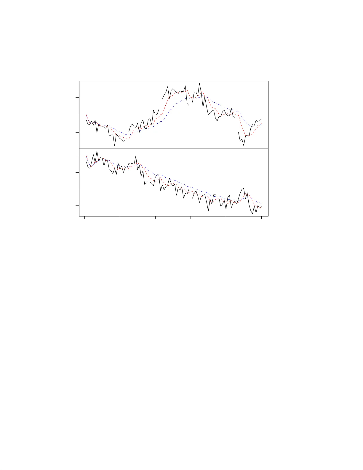
Missing observ ation analysis for matrix-v ariate time series data K. T rian tafyllop oulos ∗ Octob er 30, 2018 Abstract Bay esian inference is develop ed for matrix-v ariate dynamic linear models (MV-DLMs), in order to allow miss ing observ ation analysis, of a n y sub-vector or sub- matrix of the observ ation time series matrix . W e prop ose mo difications o f the inv erted Wishart and matrix t distributions, repla cing the scala r degrees o f freedom by a diagona l matrix of degrees of freedom. The MV-DLM is then re-defined and mo difications of the up da ting algorithm for missing observ ations are suggested. Some key wor ds: B ayesian forecasting, dynamic mo dels, in verted Wishart distributio n, state s pace mo dels. 1 In tro duction Supp ose that, in the n otat ion of W est and Harrison (1997, Chapter 16), the p × r matrix- v ariate time series { y t } f ollo ws a matrix-v ariate dynamic linear mo del (MV-DLM) so that y ′ t = F ′ t Θ t + ǫ ′ t and Θ t = G t Θ t − 1 + ω t , (1) where F t is a d × r design matrix, G t is a d × d evo lution matrix and Θ t is a d × p state matrix. Conditional on a p × p cov ariance matrix Σ, the inno v ations ǫ t and ω t follo w , resp ectiv ely , matrix-v ariate normal distrib utions (Da wid, 1981 ), i.e. ǫ t | Σ ∼ N r × p (0 , V t , Σ) and ω t | Σ ∼ N d × p (0 , W t , Σ) . This is equiv alen t to writing v ec( ǫ t ) | Σ ∼ N r p (0 , Σ ⊗ V t ) and vec( ω t ) | Σ ∼ N dp (0 , Σ ⊗ W t ), where v ec( . ) d enotes the column stac king op erator of a matrix, ⊗ denotes the K r onec ker pro du ct of t w o matrices an d N r p ( ., . ) denotes the multiv ariate n ormal distribution. ∗ Department of Probabilit y and Statistics, Un iv ersit y of Sheffield, S heffield S3 7RH, U K , email: k.triantaf yllopoulos@ sheffield.ac.uk 1 W e assume that the in no v ation series { ǫ t } and { ω t } are inte rnally and mutually uncorre- lated and also they are un correlate d with the assumed initial p riors Θ 0 | Σ ∼ N d × p ( m 0 , P 0 , Σ) and Σ ∼ I W p ( n 0 , n 0 S 0 ) , (2) for some kno wn m 0 , P 0 , n 0 and S 0 . Here Σ ∼ I W p ( n 0 , n 0 S 0 ) denotes the in v erted Wishart distribution with n 0 degrees of f reedom an d parameter matrix n 0 S 0 . The co v ariance matrices V t and W t are assumed known; usually V t = I r (the r × r identit y matrix) and W t can b e sp ecified us ing discount factors as in W est and Harrison (1997, Chapter 6). Alternativ ely , W t = W ma y b e considered time-inv ariant and it can b e estimated from the data us in g th e EM algorithm (Dempster et al. , 1977; Shum w a y and Stoffer, 1982). With the ab o v e initial priors (2) the p osterior distrib ution of Θ t | Σ , y 1 , . . . , y t is a matrix-v ariate normal distribu tion and the p osterior distribu tio n of Σ | y 1 , . . . , y t is an in v erted Wishart distribu tion with degrees of freedom n t = n t − 1 + 1 and a parameter matrix n t S t , w hic h are calculated r ecurren tly (W est and Harr ison, 1997, Chapter 16). Missing d ata in time series are typical ly handled b y ev aluating the lik eliho o d function (Jones, 1980; Lj ung, 1982; Shum wa y and Stoffer, 1982; Harvey and Pierse, 1984; Wincek and Reinsel, 1984; Kohn and Ansley , 1986; Ljung, 1993; G´ omez and Mara v all, 1994; Luce ˜ no, 1994; Luce ˜ no, 1997). In the con text of mo del (1) a ma jor obstacle in inference is when a sub -vect or or su b-matrix e y t of y t is missin g at time t . T h en the scalar degrees of fr eedom of the inv erted Wishart distribution of Σ | y 1 , . . . , y t , are incapable to include the inform atio n of the observe d part of y t , but to exclude th e influ ence of the missing part e y t . F or example consider p = 2 and r = 1 or y t = [ y 1 t y 2 t ] ′ and supp ose that at time t , y 1 t is m iss ing ( e y t = y 1 t ), w hile y 2 t is observe d. Let n t − 1 denote the degrees of freedom of the inv erted Wish art distribution of Σ | y 1 , . . . , y t − 1 . One question is how one should up date n t , since the information at time t is partial (one comp onen t observe d and one missing). Lik ewise, giv en this partial information at time t , another qu estio n is ho w to estimate the off-diagonal element s of Σ, wh ic h leads to the estimation of the cov ariance of y 1 t and y 2 t . In this p aper, in tro ducing sev eral degrees of freedom that form a diagonal matrix, w e prop ose mo difications to the inv erted Wishart and matrix t d istributions. W e prov e the conjugacy b et w een these distributions and w e discuss m o difications in the recur s ions of the p osterior moment s in the presence of missing d ata . Th is approac h do es not requir e to order all missing obs er v ations in one matrix (Shum w a y and Stoffer, 1982; Luce ˜ no, 1997) and th erefore it can b e applied for sequentia l purp oses as new data are observ ed. 2 2 Matrix-v ariate dynamic linear mo dels 2.1 Mo dified inv erted Wishart distribution Supp ose that Σ is a p × p r andom cov ariance matrix, S, R are p × p co v ariance matrices and N is a p × p d iago nal matrix with p ositiv e d iag onal element s. Let tr( . ), etr( . ) and | . | denote the trace, the exp onent of the trace and the determinant of a square matrix, resp ectiv ely . The densit y of th e inv erted Wishart d istribution is giv en b y p (Σ) = c | R | ( k − p − 1) / 2 | Σ | − k / 2 etr  − 1 2 R Σ − 1  , (3) from w hic h it is dedu ced that Z Ω | Σ | − k / 2 etr  − 1 2 R Σ − 1  d Σ = c − 1 | R | − ( k − p − 1) / 2 , (4) with Ω = { Σ ∈ R p × p : Σ > 0 } , c − 1 = 2 ( k − p − 1) p/ 2 Γ p { ( k − p − 1) / 2 } , and k > 2 p , where Γ p ( . ) is the multiv ariate gamma function. Lemma 1. The function p (Σ) = c | Σ | −{ v + tr ( N ) / (2 p ) } etr  − 1 2 N 1 / 2 S N 1 / 2 Σ − 1  , (5) wher e c do es not dep end on Σ , is a density function. Pr o of. I f the follo wing bijectiv e transf orm atio n is applied R = N 1 / 2 S N 1 / 2 and k = 2 v + tr( N ) p , (6) then (5 ) is directly obtained fr om (3). F rom the ab o v e bijection and the Wishart integral, w e can see that the norm alizing con- stan t c is c = c 0 | S | { 2 v +tr( N ) /p − p − 1 } / 2   p Y j =1 n j   { 2 v +tr( N ) /p − p − 1 } / 2 , where c − 1 0 = 2 { 2 v +tr( N ) /p − p − 1 } p/ 2 Γ p  2 v + tr ( N ) /p − p − 1 2  , for N = diag( n 1 , . . . , n p ) and n i > 0 ( i = 1 , . . . , p ). Densit y (5) prop oses a mo dification of the in v erted Wishart distribu tion in ord er to in- corp orate a diagonal matrix of d egree s of freedom. Th e mo dification consists of a bijectiv e transform of the tw o distribu tio ns. W e will then sa y that Σ follo ws the mo difie d inverte d 3 Wishart distr ib ution and we will write Σ ∼ M I W p ( S, N , v ), wh ere v is a scalar hyp erparam- eter. Note that wh en n 1 = · · · = n p = n and v = p , the ab o v e distrib u tion red uces to an in v erted Wishart distribution with n degrees of f r eedom. With k and R as defined in equation (6), the mean of Σ is E (Σ) = R k − 2 p − 2 =  tr ( N ) p + 2 v − 2 p − 2  − 1 N 1 / 2 S N 1 / 2 , for p − 1 tr( N ) > 2 p − 2 v + 2. The next result giv es the distribution of a M I W matrix conditional on a norm al matrix. Prop osition 1. L e t Y b e an r × p r ando m matrix that fol lo ws a matrix normal distribution, c onditional on Σ , and Σ a p × p c ovarianc e r andom matrix that fol lows a mo difie d inverte d Wishart distribution, written Y | Σ ∼ N r × p ( m, P , Σ) and Σ ∼ M I W p ( S, N , v ) r esp e ctively, for some known qu antities m , P , S , N , and v . Then, the c onditional distribution of Σ given Y , is Σ | Y ∼ M I W p ( S ∗ , N ∗ , v ) , wher e N ∗ 1 / 2 S ∗ N ∗ 1 / 2 = ( Y − m ) ′ P − 1 ( Y − m ) + N 1 / 2 S N 1 / 2 and N ∗ = N + r I p . Pr o of. F orm the joint distribu tion of Y and Σ and wr ite p (Σ | Y ) ∝ p ( Y , Σ) = p ( Y | Σ) p (Σ) ∝ | Σ | −{ v + r/ 2+tr( N ) / (2 p ) } etr  − 1 2 { ( Y − f ) ′ Q − 1 ( Y − f ) + N 1 / 2 S N 1 / 2 } Σ − 1  , (7) whic h is sufficien t for the pr oof with the d efi nition of S ∗ and N ∗ . In the con text of Prop osition 1 the join t distr ibution of Y and Σ is referred to as join t nor- mal mo dified inv erted Wishart d istribution with notation Y , Σ ∼ N M I W r × p,p ( m, P , S, N , v ), for m , P , S , N , and v as defined in Prop osition 1. The next resu lt giv es the marginal distribution of Y . First w e giv e some backg round material on the matrix t distrib u tion. Let X b e an r × p rand om matrix. Then, th e matrix t distribu tion is defi ned by p ( X ) = c | Q + ( X − M ) ′ P − 1 ( X − M ) | − ( k + r + p − 1) / 2 , (8) with c = Γ p { ( k + r + p − 1) / 2 }| Q | ( k + p − 1) / 2 | P | − p/ 2 π r p/ 2 Γ p { ( k + p − 1) / 2 } , where M is an r × p matrix, P a r × r co v ariance matrix, Q a p × p co v ariance matrix, and k any p ositive real num b er. 4 Prop osition 2. L et Y b e an r × p r andom matrix that fol lo ws a matrix normal distribution c onditional on Σ , and Σ b e a p × p c ovarianc e r andom matrix that fol lows a mo difie d inverte d Wishart distribution, written Y | Σ ∼ N r × p ( f , Q, Σ) , and Σ ∼ M I W p ( S, N , v ) r esp e ctively, for known quantities f , Q , S , N , and v . Then, the mar ginal distribution of Y is p ( Y ) = c | N 1 / 2 S N 1 / 2 + ( Y − f ) ′ Q − 1 ( Y − f ) | −{ 2 v + tr ( N ) /p + d − p − 1 } / 2 , (9) which by analo gy of the M I W distribution, is a mo dific ation of the matrix t distribution and it is written as M T ( f , Q, S, N , v ) . Pr o of. T he join t d istribution of Y and Σ is giv en by equation (7). Hence, the marginal distribution of Y is p ( Y ) = Z Ω p ( Y , Σ) d Σ , where Ω = { Σ ∈ R p × p : Σ > 0 } . Set R = ( Y − f ) ′ Q − 1 ( Y − f ) + N 1 / 2 S N 1 / 2 and k = 2 v + r + tr( N ) /p and from equation (4) we ha v e equ ati on (9). The distribution of Prop osition (2) can b e deriv ed from the matrix t distrib ution (see equation (8 )). The normalizing constan t c of (9) is obtainable from (8) as c = π pr / 2 Γ p { ( k + p − 1) / 2 } Γ p { ( k + r + p − 1) / 2 } | S | ( k + p − 1) / 2   p Y j =1 n j   ( k + p − 1) / 2 | Q | − p/ 2 , where N = diag( n 1 , . . . , n p ) and k = 2 v − 2 p + tr( N ) /p . Note that if all the diagonal elemen ts of N are the same (i.e. n 1 = · · · = n p = n ) an d v = p , then th e ab ov e distribution reduces to a m atrix t distribution w ith n degrees of fr eedom. Finally we giv e the m arginal distribution of Σ. Consider the follo wing partition of Σ, S , and N Σ = " Σ 11 Σ 12 Σ ′ 12 Σ 22 # , S = " S 11 S 12 S ′ 12 S 22 # , N = " N 1 0 0 ′ N 2 # , where Σ 11 , S 11 and N 11 ha v e dimension q × q , for some 1 ≤ q < p . The n ext r esult giv es the marginal d istribution of Σ 11 . Prop osition 3. If Σ ∼ M I W p ( S, N , v ) , under the ab ove p artition of Σ the distribution of Σ 11 is Σ 11 ∼ M I W q ( S 11 , N 11 , v 1 ) , wher e v 1 = v − p + q + 2 − 1 p − 1 tr ( N ) − 2 − 1 q − 1 tr ( N 1 ) . Pr o of. T he pro of su gge sts the adoption of transform atio n (6) together with the partition of R in (3) as R = " R 11 R 12 R ′ 12 R 22 # . 5 Using marginalizatio n prop erties of the inv erted Wishart d istribution, up on noticing N 1 / 2 S N 1 / 2 = " N 1 / 2 1 S 11 N 1 / 2 1 N 1 / 2 1 S 12 N 1 / 2 2 N 1 / 2 2 S ′ 12 N 1 / 2 1 N 1 / 2 2 S 22 N 1 / 2 2 # , w e get Σ 11 ∼ M I W q ( S 11 , N 1 , v 1 ), w ith v 1 as required. A similar resu lt can b e obtained for Σ 22 . Consequent ly , if w e write Σ = { σ ij } (1 ≤ i, j ≤ p ) and N = d iag( n 1 , . . . , n p ), then the d iago nal v ariances σ ii follo w mo dified inv erted Wishart distributions, σ ii ∼ M I W 1 ( s ii , n i , v i ), w here v i = v − p + 1 + 2 − 1 p − 1 tr( N ) − 2 − 1 n i . T hese in fact are inv erted gamma distribu tions σ ii ∼ I G ( v i + n i / 2 − 1 , n i s ii / 2). Note that if n 1 = · · · = n p = n and v = p , then w e ha v e that σ ii ∼ I G ( n/ 2 , ns ii / 2) (the in v erted gamma distribution used in W est and Harrison (1997) wh en p = 1). W e close this s ection with a brief discussion on an earlier stud y pr oposin g the incorp ora- tion of sev eral degrees of freedom f or in v erted Wishart matrices (Bro wn e t al. , 1994). This approac h is b ased on b reaking the degrees of freedom on b loc ks and requiring for eac h blo c k the marginal density of the co v ariance matrix to follo w an inv erted Wishart distribution. Ho w ev er, in that fr amew ork the conjugacy b et w een the normal and that distribution is lost and as a resu lt the prop osed estimation pr o cedure may b e slo w and probably n ot suitable for time series application. Relev an t inferen tial issues of that approac h are d iscu ssed in Garth- w aite and Al-Awa dhi (2001). Our prop osal of the M I W distrib ution retains the desired conjugacy and it leads to r ele v ant mo difications of the matrix t distribu tion, w hic h pro vides the forecast distribution. F urthermore, the M I W dens it y leads to fast computationally effi- cien t algorithms, which are su itable for s equen tial mo del monitoring and exp ert in terv en tion (Salv ador and Gargallo, 2004). Finally , according to Prop osition 3, the marginal distrib utions of M I W matrices are also M I W , which means that sev eral d egree s of freedom are includ ed in the m arginal mo dels to o, somethin g that is not the case in the appr oac h of Bro wn et al. (1994 ). 2.2 Matrix-v ariate dynam ic linear mo dels revisited W e consider mo del (1), b ut n o w we replace the initial priors (2) b y the priors Θ 0 | Σ ∼ N d × p ( m 0 , P 0 , Σ 0 ) and Σ 0 ∼ M I W p ( S 0 , N 0 , p ) , (10) for some kn o wn m 0 , P 0 , S 0 and N 0 . Practical ly we hav e replaced the inv erted Wishart p rior b y the M I W and so, f or eac h t = 1 , . . . , T , we use p degrees of freedom n 1 t , . . . , n pt in order to estimate Σ | y t , w here y t denotes the in formation s et, compr ising of obs erv ed data y 1 , . . . , y t . The n ext result provides th e p osterior and f oreca st distribu tions of the new MV-DLM. 6 Prop osition 4. One-step for e c ast and p osterior distributions in the mo del (1) with the initial priors (10), ar e g iven, for e ach t , as fol lows. (a) Posterior at t − 1 : Θ t − 1 , Σ | y t − 1 ∼ N M I W d × p,p ( m t − 1 , P t − 1 , S t − 1 , N t − 1 , p ) , for some m t − 1 , P t − 1 , S t − 1 and N t − 1 . (b) Prior at t : Θ t , Σ | y t − 1 ∼ N M I W d × p,p ( a t , R t , S t − 1 , N t − 1 , p ) , wher e a t = G t m t − 1 and R t = G t P t − 1 G ′ t + W t . (c) One-step for e c ast at t : y ′ t | Σ , y t − 1 ∼ N r × p ( f ′ t , Q t , Σ) , with mar ginal: y ′ t | y t − 1 ∼ M T r × p ( f ′ t , Q t , S t − 1 , N t − 1 , p ) , wher e f ′ t = F ′ t a t and Q t = F ′ t R t F t + V t . (d) Posterior at t : Θ t , Σ | y t ∼ N M I W d × p,p ( m t , P t , S t , N t , p ) , with m t = a t + A t e ′ t , P t = R t − A t Q t A ′ t , N t = N t − 1 + r I p , N 1 / 2 t S t N 1 / 2 t = N 1 / 2 t − 1 S t − 1 N 1 / 2 t − 1 + e t Q − 1 t e ′ t , A t = R t F t Q − 1 t , and e t = y t − f t . The p roof of this result follo ws immediately fr om Prop ositions 1 and 2. F or t = 1, (a) coincides with the priors (10). F rom Pr op osition 2, the m arginal p osterior of Θ t | y t is Θ t | y t ∼ M T d × p ( m t , P t , S t , N t , p ). Thus th e ab ov e prop osition giv es a recursive algorithm f or the estimation and forecasting of th e s y s tem for all t = 1 , . . . , T . Prop osition 4 gives a generalization of the up dating recursions of matrix-v ariate d ynamic mo dels (W est and Harrison, 1997, C hapter 16). Th e main difference of th e t w o algorithms is that the scalar degrees of freedom n t of the standard recursions are rep laced by N t in the ab o v e prop osition and that the inv erted Wishart distribu tion is replaced by the mo dified in v erted Wishart distr ib ution (in ord er to accoun t for the matrix of d egree s of freedom). As a result the classical Ba y esian up d ating of W est and Harrison (1997) is obtained as a s p ecia l case of the distribu tional results of Prop osition 4, b y setting N t = n t I p = diag( n t , . . . , n t ) ( t = 0 , 1 , . . . , T ), wher e n t represent the scalar degrees of freedom of the inv erted Wishart distribution of Σ t | y t and n 0 is the initial degrees of freedom. 3 Missing observ ations In this section we consider missing observ ations at random. Our approac h is b ased on ex- cluding any m iss ing v alues of the calculation of the up dating equations (state and forecast 7 distributions) thus excluding the un kno w n influ ence of these un observ ed v ariables. Th is ap- proac h is explained for univ ariate dynamic mod els in W est and Harrison (1997, Chapters 4,10). The u n iv ariate dynamic linear mo del with unkno wn observ ational v ariance is obtained from mo del (1) f or p = r = 1. In this case the p osterior recursions of m t , P t and S t of W est and Harrison (1997 , Ch apter 4) follo w from Prop osition 4 as a sp ecial case. Now su pp ose that at time t the scalar observ ation y t is missing s o that y t = y t − 1 . It is then ob vious th at the p osterior distribution of Θ t equals its p r ior distribu tion (since n o in f ormatio n comes in to th e system at time t ). Then we h a ve m t = a t , P t = R t , S t = S t − 1 and N t = n t = n t − 1 = N t − 1 . T o in corporate this in to the up dating equations of the p o sterior means and v ariances, we can write m t = a t − A t e t u t , P t = R t − A t A ′ t Q t u t , n t S t = n t − 1 S t − 1 + e 2 t u t /Q t and n t = n t − 1 + u t , where u t is zero, if y t is missing and u t = 1, if y t is observ ed. So wh en p = 1 the inclusion of u t in the p osterior recurs ions leads to identica l analysis as in W est and Harrison (1997) and in references therein. The introd u ctio n of u t in the recursions automates th e p osterior/prior up dating in the presence of missing v alues and it motiv ates th e case for p, r ≥ 1. Mo ving to the multiv ariate case, first w e consider m o del (1) as defi ned in the p revious section with r = 1. Assume that w e observ e all the p × 1 ve ctors y i , i = 1 , . . . , t − 1. A t time t some ob s erv ations are missing (sub-ve ctors of y t , or the ent ire y t ). T o d istinguish the form er from th e latter case w e hav e the f ollo wing defin itio n. Definition 1. A p artia l missing observation ve ctor is said to b e any strictly sub-ve ctor of the observation v e ctor that is missing. If the entir e observation ve ctor is missing it is r eferr e d to as fu l l missing observation ve c tor. Considering the MV-DLM (1), it is clear that in the case of a fu ll missing vecto r we h a ve Θ t , Σ | y t ∼ N M I W d × p,p ( m t , P t , S t , N t , p ) , (11) where m t = a t , P t = R t , S t = S t − 1 , N t = N t − 1 , since no inform ation comes in at time t . This equation relates to the standard p o sterior distrib ution of W est and Harr ison (1997 ) by setting N t = diag( n t , . . . , n t ), f or a scalar n t > 0 and evidently reducing the M I W distribution by a I W distribu tion. I f one starts with a pr ior N 0 = diag( n 0 , . . . , n 0 ), and assumin g that at some time t , there is a fu ll missing v ector y t , then it is clear that the p osterior (11) equ als to the p osterior of Θ t , Σ | y t using the standard recursions (W est and Harrison, 1997). An y differences b et w een the t w o algorithms is highligh ted only by obser v in g partial m issing vec tors and this has b een the motiv ation of the new algorithm. Define a p × p diagonal matrix U t = diag( i 1 t , . . . , i pt ) with i j t = ( 1 if y j t is observ ed , 0 if y j t is missing, 8 for all 1 ≤ j ≤ p , where y t = [ y 1 t · · · y pt ] ′ . Then, the p osterior distr ib ution (11 ) still applies with recurrences m t = a t + A t e ′ t U t (12) P t = R t − A t A ′ t Q t u t (13) N t = N t − 1 + U t (14) N 1 / 2 t S t N 1 / 2 t = N 1 / 2 t − 1 S t − 1 N 1 / 2 t − 1 + U t e t Q − 1 t e ′ t U t , (15) where u t = tr( U t ) /p . Some explanation for the ab o v e formulae are in order. First note that if no missing observ ation o ccurs U t = I p , u t = 1 and we ha v e th e standard recurrences as in Prop osition 4 . On the other extreme (full m iss ing ve ctor), U t = 0, u t = 0 and we hav e equation (11). Consider now the case of p artial missing observ ations. Equ ation (14) is the natural extension of the single degrees of fr eedom u p dating, see W est and Harrison (1997 , C h apter 16). F or equation (12) note that the zero’s of the main diagonal of U t con v ey the idea that the corresp onding to the missing v alues elements of m t remain unchanged and equal to a t . F or example, consider the case of p = 2, d = 2 and assume th at y ou obs er ve y 1 t , but y 2 t is missing. Then m t = a t + " A 1 t ( y 1 t − f 1 t ) 0 A 2 t ( y 1 t − f 1 t ) 0 # , where A t = [ A 1 t A 2 t ] ′ . T he zero’s on th e right hand side revea l that the second column of m t is the same as th e second column of a t . Similar commen ts apply for equations (13) and (15). Considering the case of r ≥ 2, we defi n e U k t to b e the diagonal matrix U k t = diag( i 1 k, t , . . . , i pk ,t ) with i j k ,t = ( 1 if y j k ,t is observ ed , 0 if y j k ,t is missin g, where y t = { y j k ,t } , ( j = 1 , . . . , p ; k = 1 , . . . , r ). Then, the moments of equation (11) can b e up d ated via m t = a t + A t e ′ t r Y k =1 U k t , P t = R t − A t Q t A ′ t u t , N t = N t − 1 + r X k =1 U k t N 1 / 2 t S t N 1 / 2 t = N 1 / 2 t − 1 S t − 1 N 1 / 2 t − 1 + r Y k =1 U k t ! e t Q − 1 t e ′ t r Y k =1 U k t ! , where u t = tr( Q r k =1 U k t ) /p . Similar comment s as in the case of r = 1 apply . Definition 1 is trivially extended in th e case when obs er v ations form a matrix ( r ≥ 2). W e illustrate the prop osed metho dology by consider in g simulat ed data, consisting of 100 biv ariate time series y 1 , . . . , y 100 , generated from a lo cal level mo del y t = [ y 1 t y 2 t ] ′ = ψ t + ǫ t and ψ t = ψ t − 1 + ζ t , wh ere ψ 0 , ǫ t and ζ t are all simulat ed from biv ariate n ormal d istributions. The 9 −5 0 5 −15 −10 −5 0 0 20 40 60 80 100 Forecast mean Time y 1 y 2 Figure 1: Sim ulated biv ariate time series (soli d line) with one-ste p forecasts from (a) the standard DLM recursions (dotted/dashed line) and (b) the new DLM recursions (dashed line). The gaps indicate missing v alues. correlation of ǫ 1 t and ǫ 2 t is set to 0 . 8, while the elemen ts of ζ t are uncorr elated. This mo del is a sp ecial case of mo del (1) with Θ ′ t F t = ψ t and G t = I 2 . Figure 1 (solid line) shows the sim ulated data; the gaps in this figur e indicate missing v alues at times t = 24 , 43 , 60 , 75 , 86. A t times t = 24 , 43 , 86, y t 2 is on ly missin g (partial missing ve ctors), at time t = 75, y t 1 is only missing (partial missing ve ctor) and at time t = 60, b oth y t 1 , y t 2 are m issing (full miss in g v ector). F or this data set, w e compare the p erf ormance of recur s ions (12)-(15) with that of the classic or old recursions of W est and Harrison (1997), wh ic h assume that wh en there is at least one miss ing v alue we set U t = 0 and u t = 0. F or example using th e old recurs ions , for t = 24 one wo uld set U 24 = 0 and u 24 = 0, losing the “partial” information of y 24 , 1 = − 3 . 739, whic h is observ ed. O n the other hand, the new r ecursions would suggest for t = 24 to set U 24 = " 1 0 0 0 # and u 24 = 1 / 2 . Figure 1 shows the one-step forecast m ean of { y t } u sing the new r ecursions (dashed line) and the old recursions (dotted/dashed line). W e observ e th at th e n ew metho d pro duces a clear improv ement in the forecasts as the old r ecur sions p ro vide p o or forecasts, esp ecially in 10 the lo w panel of Figure 1 (for { y 1 t } ). What is really happ enin g in this case is that, und er the old recursions, the missing v alues of y 2 t affect the recursions for y 1 t , since th e observed information at y 1 t is wrongly “masked” or “ignored” for the p oin ts of time when y 2 t is missin g. On the other hand, th e new recurs ions use th e explicit in f ormatio n fr om eac h sub -v ector of y t and thus the new recur sions result in a n ota bly more accurate forecast p erform ance. T his is bac k ed b y th e mean squ are standard ized forecast error vect or, whic h for th e new r ecursions is [1 . 300 1 . 825] ′ , wh ile for the old r ecursions is [1 . 545 2 . 182] ′ . Un der the old recur s ions we can not obtain an estimate of the co v ariance b et w een an observed y 1 t and a missing y 2 t . How eve r, this is in deed obtained un d er th e p rop osed n ew recursions and so the resp ectiv e correlations at p oin ts of time where there are gaps are 0 . 63 3 (at t = 24), 0 . 779 (at t = 43), 0 . 812 (at t = 75) and 0 . 809 (at t = 86); the mean of these correlatio ns is 0 . 792, wh ic h is close to th e real 0 . 8 un der th e simulat ion exp eriment . Ac kno wledgemen ts I am grateful to Jeff Harr ison for us efu l discus sions on the topic of missing d ata in time ser ies. I would lik e to thank a referee for helpful comments. References [1] Bro wn, P .J., Le, N.D. and Zidek, J.V. (1994) I nference for a co v ariance matrix. In Asp e cts of U nc ertainty (eds P .R. F r eeman, A.F.M. S mith). Chic hester: Wiley . [2] Da w id, A.P . (1981), Some m atrix-v ariate distribution theory: notational considerations and a Ba y esian app lica tion, Biometrika , 68 , 265-274. [3] Dempster, A.P ., Laird , N.M. and Rubin, D.B. (1977) Maximum lik elihoo d fr om incom- plete data via the EM algorithm (with discussion). Journal of the R oyal Statistic al So ciety Series B , 39 , 1-38. [4] Garth w aite, P .H. and Al-Awa dhi, S .A. (2001) Non-conjugate prior distrib u tion assess- men t f or multiv ariate normal sampling. Journal of the R oyal Statistic al So ci e ty Se rie s B , 63 , 95-110. [5] G´ omez, V. and Marv all, D. (1994) Estimation, p rediction, an d interp olat ion for nonsta- tionary series with th e Kalman filter. Journal of the Americ an Statistic al A sso ci atio n , 89 , 611-624. 11 [6] Harv ey , A.C. and Pierse, R.G. (1984) Estimating missing obs erv ations in economic time series. Journal of the Americ an Statistic al Asso ciation , 79 , 125-131. [7] Jones, R.H. (198 0) Maxim um lik elihoo d fi tting of ARMA mo dels to time series with missing obser v ations. T e chnometrics , 22 , 125-131. [8] Kohn, R. and Ansley , C.F. (1986) Estimation, pred iction, and interp olation for ARIMA mo dels with miss in g obs er v ations. Journal of the Americ an Statistic al Asso ciation , 81 , 751-7 61. [9] Ljung, G.M. (1982) The lik eliho od fun ctio n of a stationary Gaussian autoregressiv e- mo ving-a verag e pro cess with m issing observ ations. Biometrika , 69 , 265-268. [10] L j ung, G.M. (1993) On outlier detection in time series. Journal of the R oyal Statistic al So ciety B , 55 , 559-56 7. [11] L u ce˜ no, A. (1994 ) A f ast algorithm for the exact likel iho o d of stationary and p artial ly nonstationary v ector autoregressiv e mo ving a v erage pro cesses. Biometrika , 81 , 555-565. [12] L u ce˜ no, A. (1997) Estimation of missing v alues in p ossibly partially nonstationary ve ctor time ser ies. Bi ometrika , 84 , 495-499. [13] S alv ad or, M. and Gargallo, P . (2004). Automatic monitoring and interv ention in m ulti- v ariate d ynamic linear mo dels. Computatio nal Statistics and Data Analysis , 47 , 401-4 31. [14] S h um w a y , R.H. and Stoffer, D.S. (1982) An approac h to time series smo othing and forecasting using the EM algorithm. Journal of Time Series Analysis , 3 , 253-264. [15] W est, M. and Harrison, P .J. (1997) Bayesian F or e c asting and Dynamic M o dels , S p ringer- V erlag (second edition), New Y ork. [16] Wincek, M.A. and Reinsel, G.C. (1986) An exact maxim um likel iho o d estimation pro ce- dure for regression-ARMA time series m odels with p ossibly n onconsecutiv e d ata. Journal of the R oyal Statistic al So ciety B , 48 , 303-313 . 12