Analytical Solution of Covariance Evolution for Regular LDPC Codes

Amraoui [3] showed that distributions of the number of check nodes of degree one in the residual graph convergences weakly to a Gaussian as blocklength tends to infinity. Amraoui also showed that block and bit error probability of finite-length LDPC codes are derived by the average and the variance of the number of check nodes of degree one in the residual graph. The average number of check nodes of degree one in the residual graph is determined from a system of differential equations, which was derived and solved by Luby et al. [2]. The variance of the number of check nodes of degree one in the residual graph is also determined from a system of differential equations called covariance evolution, which was derived by Amraoui et al. [3]. Since analytical solution of covariance evolution has not been known so far, we had to resort to numerical computations to solve the covariance evolution.

An alternative way to determine the variance of the number of check nodes of degree one was proposed in [3]. The variance of the number of check nodes of degree one in the residual graph can be computed by determining the variance of the number of erased messages of BP for BEC with parameter ǫ * where ǫ * is the threshold of the ensemble under BP decoding. This method is a valid approximation for the erasure probability close to ǫ * . Moreover, Ezri et al. extended to this method to more general channels [5]. However, if we solve the covariance evolution analytically, we can derive the variance of the number of check nodes of degree one in the residual graph for all ǫ where ǫ is the channel parameter for the BEC.

In this paper, we show an analytical solution of the covariance evolution for regular LDPC code ensembles. [3] In this section, we briefly review the covariance evolution and initial covariance in [3].

We consider the transmission over the BEC with channel erasure probability ǫ using LDPC codes in a (b, d)-regular LDPC code ensemble. Let t denote the iteration round and ξ be the total number of edges in the original graph. We define that

Define a parameter y such that dy/dτ = -1/(ǫy b-1 ) and y = 1 when τ = 0. Let l b,t denote a random variable corresponding to the number of edges connecting to variable nodes of degree b in the residual graph at the iteration round t. Let r k,t denote a random variable corresponding to the number of edges connecting to check nodes of degree k in the residual graph at the iteration round t. Those random variables depends on the choice of the graph from (b, d)-regular LDPC code ensemble, the channel outputs and the random choices made by PA. We define

To simplify the notation, we drop the subscript t. For i ∈ D t , we define ī(y) by

We also define δ (i,j) (y) by the covariance of i and j (i, j ∈ D t ) divided by the total number of edges in the original graph i.e.

In [3], Amraoui showed these parameters satisfy the following system of differential equations in the limit of the block length.

This system is referred to as covariance evolution.

where

) and I {k=s} is the indicator function which equals to 1 if k = s and 0 otherwise.

The initial conditions of the covariance evolution are given by initial covariances. The initial covariances are the covariances of the number of edges of each degree at the start of the decoding divided by the total number of edges in the original graph. For j, k ∈ {1, 2, . . . , d}, initial covariances are derived in [3], as follows.

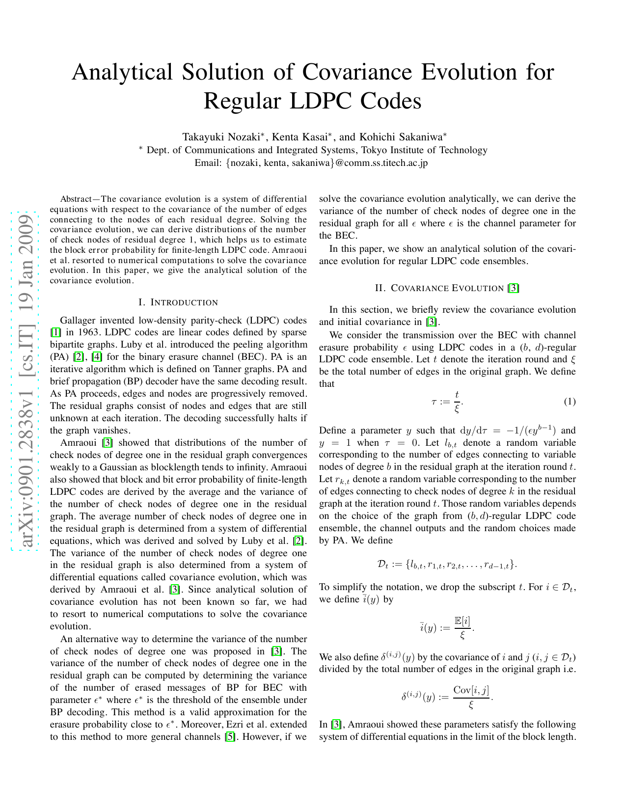
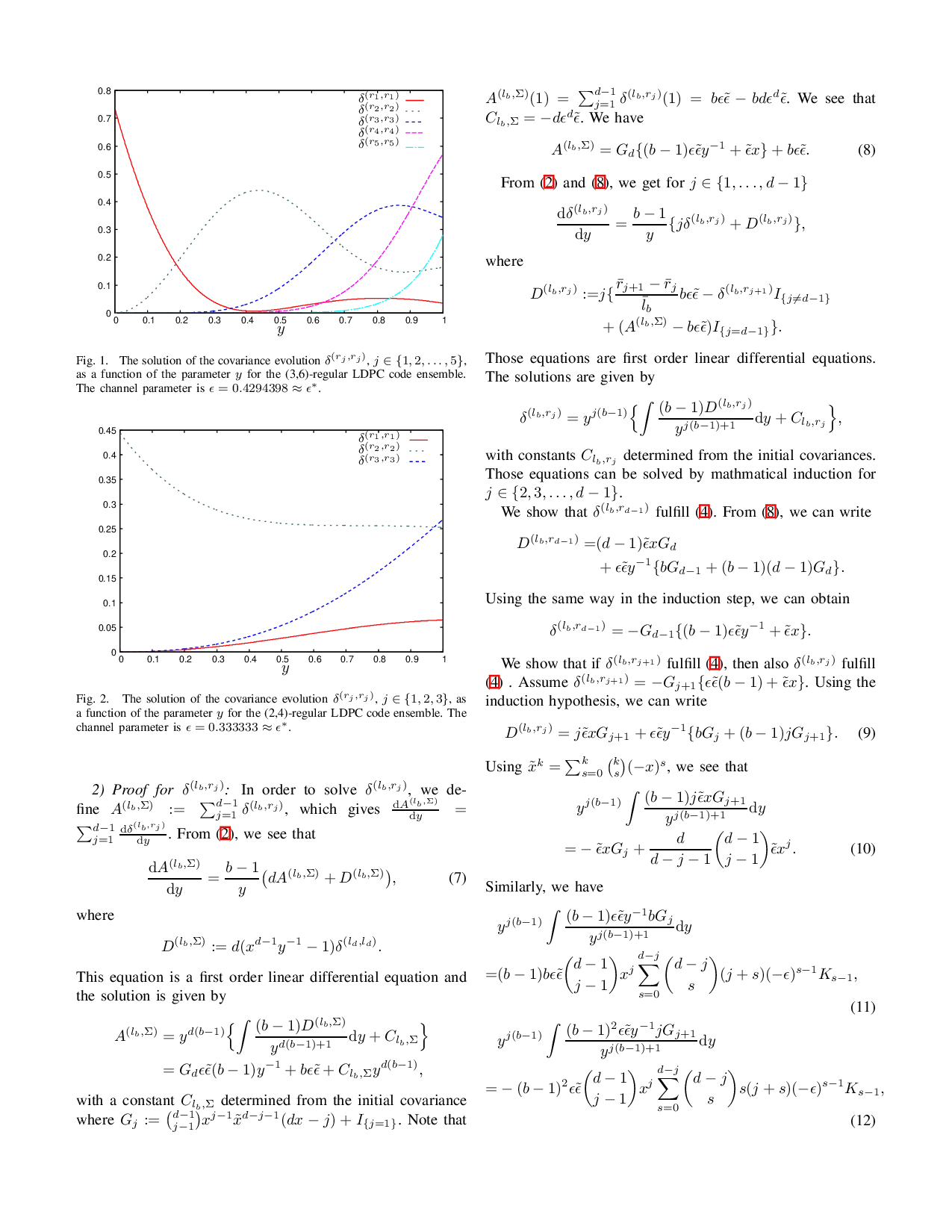
We show in the following theorem the analytical solution of the covariance evolution, for a (b,d)-regular LDPC code ensemble. The proof1 is given in Section III-C. Theorem 1. Let τ be the normalized iteration round of PA as defined in (1). For a (b,d)-regular LDPC code ensemble and j, k ∈ {1, 2, . . . , d -1}, in the limit of the code length, we obtain the following.

where G j := d-1 j-1 x j-1 xd-j-1 (dx -j) + I {j=1} and y is defined by dy/dτ = -1/(ǫy b-1 ) with y = 1 when τ = 0.

In [3], scaling parameter α is given by

where ǫ * is the threshold of the ensemble under BP decoding , y * is the non-zero solution of r1 (y) at the threshold , n is the blocklength and ξ is the total number of edges in the original graph.

We define x * := ǫ * (y * ) b-1 and x * := 1 -x * . Since r1 (ǫ * , y * ) = 0 and ∂ r1 ∂y | ǫ * ;y * = 0, we see that

. Using those equations, we have from ( 5)

Recall that r1 (ǫ, y) = x(y -1 + xd-1 ). We see that ∂r 1 ∂ǫ y * ;ǫ * = -

.

F

…(Full text truncated)…