Degrees of Freedom of a Communication Channel: Using Generalised Singular Values

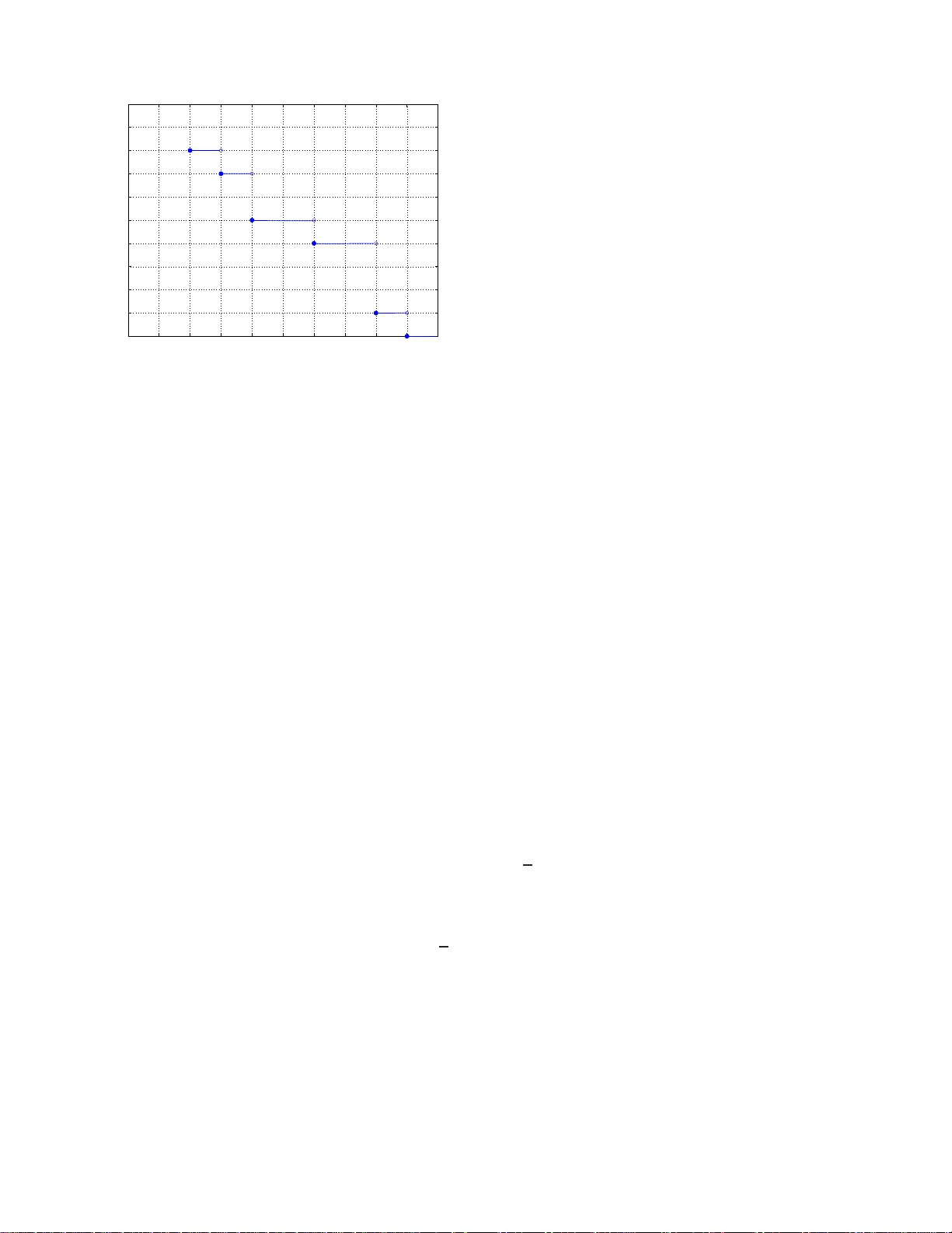
De grees of Freedom of a Commun icati on Channel: Using Generalised Singular V alues Ram Somaraju and Jochen T rumpf Abstract A fundam ental problem in any co mmun ication system is: given a comm unication chan nel between a transmitter and a r eceiv er, how many “independent” signals can be exchanged between them? Arb itrary commu nication channels that can be described by linear co mpact channel ope rators mapping between no rmed spaces are examined in this paper . The (well-kn own) notio ns of degrees of freedom at level ǫ and essential dimension o f such ch annels are developed in this general setting . W e a rgue th at the degrees o f fr eedom at level ǫ and the essential d imension fundam entally limit the numbe r of in depen dent signals that can be exchang ed b etween the tran smitter and the receiver . W e also generalise the concep t o f singular values of compact o perator s to be applicable to compac t operator s defined on ar bitrary normed sp aces which d o not nec essarily c arry a Hilber t space structu re. W e show how these gener alised sing ular v alues can be used to calcula te the degrees of freedom at le vel ǫ an d the essential dimension of comp act oper ators that describe communica tion channels. W e describe physically re alistic channels that requ ire such general channel mo dels. Index T erms Operator Chan nels, Degrees of Freedom, Generalised Sing ular V alues, Essential Dim ension 1 De grees of Freedom of a Commun icati on Channel: Using Generalised Singular V alues I . I N T RO D U C T I O N The basic co nsideration in this paper can be stated a s follo ws: given a n arbitrary communica tion c hanne l, is it possible to evaluate the numbe r of inde pende nt sub- channe ls or modes available for commun ication. Thou gh this question is not generally examined e xplicitly , it plays an impo rtant role in various informati on theoretic problems. A rigorous proof of Sh annon’ s famous ca pacity re- sult [1] for continuous-time ban d-limited white Gauss ian noise ch annels requires a calculation of the number of approximately time-limited and ban d-limited sub- channe ls (see e .g. [2, ch. 8] a nd [3, 4]). T his res ult c an be generalised to dispersive/non-white Gaus sian channels using the water-filling formula [1,2]. In order to us e this formula, one needs to diago nalise the c hanne l operator and alloca te power to the different sub -channe ls or modes base d on the singu lar values of the correspon ding sub-chan nel. One therefore needs to calculate the mode s and the power transferred (square o f the sing ular values) on eac h one of thes e sub-chan nels to calculate the channe l capacity . The water -filling formula has been used extensi vely in order to calculate the cap acity of cha nnels that use dif ferent forms of diversity . In pa rticular , the c apacity of multiple-input multiple-output (MIMO) an tenna sy stems has be en calc ulated using this water -filling formula for various c onditions imposed on the transmitting and the receiving antennas (se e e.g. [5] and referen ces the rein). W ater- filling t ype formulas hav e b een us ed for other multi-access sc hemes such as OFDM-MIMO [6] and CDMA [7] (see also T ulino [8, sec 1.2] and references therein). More recently , sev eral papers have examined the number of degrees of freedom 1 av ailable in s patial channe ls [9]–[13]. Que stions of this nature ha ve also been stud ied in other contexts such a s o ptics [14] and spatial sampling of elec tromagnetic wa ves [15,16]. Both types of results, the modes of communication used for the water-fill ing formula and the numb er of degrees of freedom of spatial c hanne ls use the s ingular 1 Note t hat other terms such as modes of communication , essential dimension e tc. hav e been u sed instead o f degrees of freedom in some of these papers. value decompos ition (SVD) theorem. On e can use SVD to diagonalise the ch annel op erator and the mag nitude of the singula r values determines the p ower transferred on each of t he sub-cha nnels. The magn itude of these singu- lar v alues c an therefore be used to calculate the number of degrees of freedom of the chan nel (see e.g. [9,12]). Howe ver , the SVD theorem is only applicable to compact operators d efined o n Hilbert spac es. An implicit a nd valid as sumption that is used in these papers is that the op erators d escribing the c ommunication ch annels are defined on Hilbert spaces . These results can therefore not be ge neralised directly to commun ication systems tha t are modeled by operators defined on normed spac es that do not admit an inner product structure. There are se veral instances of practical c hanne ls that ca n not be modeled using o perators d efined on inne r -produc t spac es (see Section II-A for examples). In this paper , we develop a general theory that ena bles o ne to evaluate the numbe r of degrees of freedom of suc h systems. W e wish to examine if it is poss ible to evaluate the number of pa rallel sub-chan nels available in ge neral communication systems that can be des cribed using linear c ompact opera tors. A ny communica tion c hanne l is subject to various phy sical con straints su ch a s noise at the rec eiv er or finite power av ailable for trans mission. If the c hannel c an be modeled via a linear compact op er- ator , then thes e cons traints ensure that only fi nitely many independ ent chan nels are avail able for commu nication. Roughly s peaking , we call the number of such ch annels the numb er of d egrees of freedom of the commun ication system (see Section III for a precise de finition). Note that if the chan nel is modeled using a linea r operator that is not c ompact then it will in fact have infinitely many para llel sub-cha nnels, or so me chann els that c an transfer an infinite a mount of power (se e Theorem 3.10 below and the disc ussion following it). It could he nce be argued tha t the theory presented in this paper is the most general the ory ne eded to mode l p hysically realistic channe ls. W e gi ve n ovel defin itions f or the terms degr ee s of free- dom an d ess ential dimension in the following section. Even though these terms have been use d interchang eably in the literature, we distinguish between the two. The essen tial d imension of a cha nnel is useful for c hanne ls 2 that hav e numbers of degrees of freedom that are es- sentially indepen dent of the recei ver noise lev el (e.g. the time-wi dth/ban d-width limit ed channels i n Slepian’ s work [17]). Also, we generalise the n otion of s ingular values to compa ct ope rators define d on normed s paces and explain how thes e generalised singu lar values can be us ed to c ompute degrees of freedom and the es sential dimension. A. Channe l Model W e assume that a communication channel be tween a transmitter and a receiver c an be mod eled as follows. Let X be a linear vector sp ace of functions that the transmitter ca n g enerate an d let Y be a linear vector space of functions that the receiver can meas ure. W e assume the existence of a linear operator T : X → Y that maps each signal g enerated by a transmitter to a signal that a recei ver c an measure. W e also assume tha t there is a norm k · k X on X and a norm k · k Y on Y . This model is very ge neral and c an be a pplied to various situations of practical relevance. For instance, cons ider a MIMO communica tion sy s- tem wherein the transmitter symbol wa veform shape on each a ntenna is a rais ed c osine. In this case w e ca n think of the spac e of trans mitter functions X to be (more precisely , t o be parametrised by) the n -dimensiona l com- plex space C n that determines the p hase and amplitude of the raised cos ine w aveform on each antenna. Here n is the numbe r of trans mitting antenn as. Also, we can think of the space of receiv er func tions as C m , where m is the number of recei ving antennas . T in this context is a cha nnel matrix, rep resenting the linearized channe l operator that depends on the scatterers in the en vironment. Alternati vely , cons ider a MIMO communication sys- tem in which the transmitter s ymbols are not fixed but can be any waveform of time. Suppos e the symbo l time is fixed to t s second s. In this case , we ca n think of the space of transmitter functions, X , a s the space L 2 ([0 , t s ] , C n ) of C n -valued s quare integrable fun ctions defined on [0 , t s ] . Similarly , we c an think of the space of receiver functions, Y , a s the space L 2 ([0 , t s ] , C m ) . Again, T is the channe l operator . Irrespectiv e of the precise form of the underlying space s X and Y , we always call elemen ts of X transmit- ter functions and the e lements of Y receiver functions . Also, we call the spa ce X the space o f trans mitter functions and the space Y the spac e o f receiver functions. In particular , we do not distinguis h be tween the tw o dif ferent physical situa tions: a) the elements of X are functions of time and b) the elements of X are vec tors in so me finite dimensiona l spac e. This should cau se no confusion and we use this con vention for the remaind er of this doc ument. W e now restrict ourselves to situations where there is a source constraint k · k X ≤ P that can be impos ed on the spac e of transmitter functions X , and where the operator T is co mpact. Roug hly spe aking, the no rm on the s pace o f trans mitter fun ctions X captures the physical restriction that the transmitter func tions can not be arbitrarily big , while the no rm o n the spac e o f receiv er functions can be i nterpreted as a measure of ho w big the recei ved signals are compared to a pre-spe cified noise level. W e therefore try to find h ow many linearly independ ent signals can be g enerated at the receiv er tha t are big enou gh by tr ans mitter functions that are n ot too big . The c ompactnes s of the operator T e nsures that o nly finitely many independ ent s ignals can be rec eiv ed (see Section II-A for examples of suc h cha nnels). This vague idea is clarified further in the follo wing two sections . B. Outline The remainder of this p aper is organised as follows: in the next se ction we consider a fi nite dimensional exam- ple and motiv ate the d efinition of de grees of freedom. W e also d iscuss s ev eral examples of practical c ommunica- tion s ystems to wh ich the theo ry developed in this pape r may b e a pplied. Section III p resents the main res ults of this paper as we ll as formal definitions of degrees of free dom, ess ential dimension and gene ralised s ingular values. Conc lusions are p resented i n Section IV. Detailed proofs of the theorems in this paper are prese nted in the Appendix. Most of the material p resented in this pape r forms part of the first author’ s PhD thesis [18]. I I . M OT I V A T I O N W e motiv ate o ur defin ition of degrees of freedom at level ǫ for comp act op erators on normed sp aces by considering linear operators on finite dimensional spaces . Consider a communication ch annel that u ses n transmit- ting an tennas and m receiving anten nas which ca n be mathematically modeled as follo ws. Let the c urrent on the n trans mitting antennas be given by x ∈ C n . This current on the trans mitting anten nas generates a current y ∈ C m in the m rec eiving ante nnas acco rding to the equation y = Hx . Here, H ∈ C m × n is the cha nnel matrix. W e ca n d efine the ope rator T : C n → C m by x 7→ y = H x . Also , for n = 1 , 2 , . . . , k · k = p ( · ) ∗ ( · ) , with ( · ) ∗ denoting 3 the comp lex c onjugate transpos e, is the standa rd norm in C n . In this context, the norm de termines the power of the signa l on the antenna s. The singular v alue decompos ition theorem tells us that there exist sets of o rthonormal basis vectors { v 1 , . . . , v n } ⊂ C n and { u 1 , . . . , u m } ⊂ C m such that the matrix r epres entation for T in these bases is diagona l. Let H d be such a matrix with the ba sis vectors ordered such that the diagonal elements (i.e. the singular v alue s of T ) a re in non -increasing order . A simple e xamina tion of the diagona l matrix prov es that for all ǫ > 0 there exist a number N and a s et of linea rly inde pende nt vectors { y 1 , . . . , y N } ⊂ C m such that for a ll x ∈ B 1 , C n (0) 2 inf a 1 ,...,a N      H d x − N X i =1 a i y i      ≤ ǫ. For a given ǫ , call the smallest n umber that satisfies t he above c ondition N ( ǫ ) . Note that the vectors y 1 , . . . , y N span the s pace of all linear combina tions of the left singular vectors of T who se correspond ing singular values are greater than or equal to ǫ . A simple examination of the diagonal matrix te lls us that N ( ǫ ) is equal to the numbe r of singular values of T that are greater than ǫ and is hence clearly independen t of the base s ch osen. This leads us to our defin ition for degrees of freedom in finite dimen sional spaces . Definition 2.1: Le t T : C n → C m be a linear operator and let ǫ > 0 be gi ven. Then the numbe r of degrees of freedom at le vel ǫ for T is the smallest n umber N suc h that there exists a set of vectors y 1 , . . . , y N ∈ C m such that for all x ∈ B 1 , C n (0) inf a 1 ,...,a N      T x − N X i =1 a i y i      ≤ ǫ. This definition is appropriate for the numbe r of degrees of freedo m be cause for a MIMO system the norm k · k represents the power in the signa l. Supp ose we wis h to transmit N linearly indepen dent signals from the transmitter to the r ece iv er , a nd the total po wer a vailable for transmission is b ounded . Suppos e further that the receiv ed signal is meas ured in the presenc e of n oise. By requiring tha t x ∈ B 1 , C n (0) we are constraining the power av ailable for transmission. W e mo del the noise by a ssuming tha t a ny two sign als a t the rece i ver can be distinguish ed if the p ower of the dif ference b etween the signals is greater than some level ǫ . Simil ar ideas have been use d for instance by Bucci et. al. [16 ] (se e also [4,10 ,17]). Ac cording to this defin ition, the number of degrees of freedo m is equal to the number of linearly 2 Giv en a normed space X , r ≥ 0 and x ∈ X , B r,X ( x ) de notes the closed ball of radius r centered at x ∈ X . independ ent signa ls that the receiver ca n distinguish under the assu mptions o f a transmit power c onstraint and a rece iv er nois e le vel represented by ǫ . Note that we are mak ing the implicit a ssumption tha t the power P is 1 in the ab ove defi nition. This does not cause a problem bec ause we can always scale t he norm in order to cons ider situations where P 6 = 1 . The above definition was moti vated using the singu - lar value de compos ition theorem in finite dimens ional space s. It can therefore b e easily generalised to infinite dimensional H ilbert spaces using the corresponding sin- gular v alue decompo sition in infinite dimensiona l Hi lbert space s (see eg. [16,18 ] 3 ). Howe ver , the singular v alue decompo sition can on ly be u sed for op erators d efined on Hilbert spa ces. It can not be used for o perators defin ed on general normed spac es. Observe that the definition for degrees of freedom a bove only depen ds on the norm k · k and not on the as sumption that the underlying spac es C n and C m are Hilbert spa ces. It will b e s hown in this pape r that the above definition c an be extended to co mpact operators define d on arbitrary normed space s. Now cons ider the situation wh ere the singu lar val- ues of the operator T show a step like beh av- ior . For instance, suppose the singu lar values are { 1 , 0 . 9 , 0 . 85 , 0 . 5 , 0 . 1 , 0 . 05 , . 000 5 } . In this particular c ase the number of degrees of freedom at level ǫ is equal to 4 for a big range of values o f ǫ a nd the n umber of degrees o f freedom is essentially ind epende nt o f the actual v alue of ǫ ch osen. Such a situation arises in se veral important cases (se e eg. [4,9,1 4,16,17 ]). It would b e useful to have a gene ral way in which one can specify a number o f degrees of freedom of a ch annel that is independ ent of the arbitraril y ch osen l evel ǫ . In this paper we provide a novel d efinition for suc h a numbe r a nd call it the e ssential dimension of the channe l. This definition is suf ficien tly gen eral to be applicable to a variety o f channe ls an d qu antifies the es sential dimension o f any channe l that c an be des cribed us ing a compact o perator . A. Examples As explained in section I-A, we assu me that a commu- nication channel can be d escribed using the triple X , Y and T . Here X is the space of transmitter functions, Y is the s pace of rece i ver functions and T is the ch annel operator and is ass umed to be compac t. As explained earlier in this section, if the s paces X and Y are Hilbert space s and if the o perator T is a linear compa ct operator then the well known theory o f s ingular values of Hilbert space op erators can be used to d etermine t he number o f degrees of freedom of such cha nnels. Howe ver , if either 3 Also compare with the ti me-bandwidth problem in [4,17]. 4 one of the s pace s X or Y is not an inne r product s pace then one can not use this theory . There are several practical channe ls tha t are best described using a bstract s paces that do not a dmit an inner product s tructure. In this subs ection, we cons ider three examples of such chan nels. In the first example, the me asuremen t technique used in the r ec eiv er restricts the space of receiv er functions. In the secon d on e, the modulation techn ique u sed mea ns that the co nstraints on the space of transmitter functions are best des cribed using a norm that is not compa tible with a n inner product. The fina l example discusses a physical cha nnel that naturally admits a norm on the space o f tr ans mitter functions tha t is described us ing a vector produ ct and therefore does not a dmit an inner-product structure. Example 2.1: In any practical digital commun ication system, the receiv er is designed to rec eiv e a finite set of transmitted signals. Suppose the trans mitted signal is generated from a so urce alphabet { t 1 , . . . , t N } an d for simplicity assume tha t i n a noiseless sy stem each element from the source alphabet t i , 1 ≤ i ≤ N , generates a sig- nal r i , 1 ≤ i ≤ N , at the receiver . In the corresponding noisy system, the fund amental problem is to determine which e lement from the source alph abet was transmitted giv en the sign al r = r i + n was re ceiv ed. Here, n is the noise in the sys tem. One common approach to solving this problem is to define some metric d ( · , · ) that measures the dista nce between two receiver signa ls and to calculate r ′ = argmin { r i , 1 ≤ i ≤ n } d ( r , r i ) . One c onclude s that the element from the so urce alphabet that correspon ds to r ′ is (most likely) the trans mitted sig- nal. Generally , this metric d ( · , · ) determines the abstract space Y of receiver function. Now c onsider a MIMO antenn a system with n trans- mitting and m receiving antenn as. Su ppose that the re- ceiv er meas ures the signals o n the m receiving antenn as for a period of τ seco nds. One can desc ribe the received signal by a fun ction y ( t ) , whe re y : [0 , τ ] → C m . In order to impleme nt the rece i ver one can use a matche d filter if the sha pes of all no iseless rece iv er sign als are known. In this ca se the distance betwee n two received signals can be d escribed using the metric d ( y 1 , y 2 ) =  Z τ 0 ( y 1 ( t ) − y 2 ( t )) ∗ ( y 1 ( t ) − y 2 ( t )) dt  1 / 2 One can describe the sp ace of rec eiv er functions using the Hilbert spa ce L 2 ([0 , τ ] , C m ) with the inner p roduct defined by h y 1 , y 2 i := Z τ 0 y ∗ 1 ( t ) y 2 ( t ) dt. This is the common approac h used in information theory . Howe ver , it is gene rally e asier to measu re just the amplitude of the rec eiv ed signa l on each of the m antennas . In fact, in a rap idly changing en vironmen t it might not be pos sible to build a n effecti ve matched filter and the refore there is n o benefit in me asuring the square of the recei ved s ignal. In this ca se the distance b etween any tw o sign als can be de scribed using the metric d ( y 1 , y 2 ) = Z τ 0 | y 1 ( t ) − y 2 ( t ) | dt. Here, on e can de scribe the space of receiver functions using the Ba nach spa ce L 1 ([0 , τ ] , C m ) with the norm defined by k y k := Z τ 0 | y ( t ) | dt. This channel therefore is best desc ribed using a normed space as op posed to an inner product space to mo del the set of receiver s ignals. Example 2.2: Con sider a multi-carrier c ommunica- tion system that uses s ome form of amplitude or angle modulation to trans mit information. Suppos e that the re are n carriers and that the vector φ = [ φ 1 , . . . , φ n ] determines the modulating signal on eac h of the c arriers. W e can think of the modulating waveforms as the spa ce of transmitter functions X 4 . If amplitude modulation is us ed the n the vector φ determines the total power used for modulation. If the total power av ailable for transmission is bou nded then one might have an inequality of the form n X i =1 | φ i | 2 ≤ P . W e can therefore desc ribe the s pace of transmitter func- tions using the standa rd Euc lidian space R n with inner product h x 1 , x 2 i = x T 1 x 2 . Now conside r the cas e whe re angle modulation is used. In this case all the trans mitted signals have the same power and the total p ower av ailable for trans mis- sion places no restrictions on the space o f transmitter functions. Ho wever , the space of transmitter functions can be su bjected to o ther forms of co nstraints. For instance, if frequency mod ulation is used then the ma x- imum frequen cy deviation used might be bound ed by some numb er b to minimise co-ch annel interference (se e e.g. [19, p. 110,5 13]). Simil arly if phase modulation is used the maximum pha se variati on ha s to be less than 4 In this case we do not consider the actual si gnal on the transmit- ting antenna (i.e. carrier + modulation) to be the transmitter f unction. Cf. the discussion in Subsection I-A. 5 ± π . This b ound may also de pend o n other practical considerations suc h as linearity of the modulator . In this case o ne might constrain the spac e of transmitter functions as sup 1 ≤ i ≤ n | φ i | < b. The spa ce of transmitter fun ctions of this ch annel is bes t described u sing the n -dimens ional Banac h s pace R n ∞ with norm k x k = sup 1 ≤ i ≤ n | x i | . Example 2.3: In this final example we exa mine spatial wa veform chann els (SWCs) [18]. In SWCs we ass ume that a current flows in a volume in spa ce and ge nerates an e lectromagnetic field in a rec eiv er volume that is measured [10,15 ,16,18]. Such chann els ha ve been use d to model MIMO sy stems pre viously [10,12,13 ,15,16,1 8]. If a current flows in a volume in space that ha s a finite conduc ti vity , power is lost from the transmitting volume in two forms. Firstly , po wer is lost as he at an d secon dly power is radiated a s e lectromagnetic ene rgy . So the total power lost can be described using the set of equations P total = P r ad + P lost P lost = Z V J ∗ ( r ) J ( r ) d r P r ad = Z Ω E ∗ ( r ) × H ( r ) d Ω Here, V is some volume tha t contains the transmitting antennas , J is the current d ensity in the volume V and Ω is s ome sufficiently smo oth surface the interior of whic h contains V with d Ω denoting a surface a rea element. Also E and H are the electric an d magnetic fields gen erated by the current d ensity J and · × · denotes the vector product in R 3 . Becaus e of the vector product in the last eq uation above, the total power lost defines a norm on the spa ce of s quare-integrable fun ctions tha t d oes not ad mit an inner-pr odu ct structure [18 ]. The t heo ry de veloped in this paper is used to calculate the degrees of freedom o f suc h spatial wa veform channe ls in [18]. I I I . M A I N R E S U L T S In this section we o utline the main results of this paper . All the proofs o f theorems are given in the Appendix. A. De grees o f F r eedom for Compact Operators The defi nition of degrees of freedom at level ǫ for compact operators on normed spaces is ide ntical to the finite d imensional c ounterpart (Definition 2.1) discu ssed in the previous section with C n and C m replaced b y general normed s paces . Th e following theorem ensu res that the de finition makes sense even in the infi nite dimensional setting. Theorem 3.1: Suppos e X and Y are normed spac es with norms k· k X and k· k Y , respectiv ely , and T : X → Y is a compact operator . The n for all ǫ > 0 there exist 5 N ∈ Z + 0 and a set { ψ i } N i =1 ⊂ Y such that for all x ∈ B 1 ,X (0) inf a 1 ,...,a N      T x − N X i =1 a i ψ i      Y ≤ ǫ. Note that for N = 0 the se t { ψ i } N i =1 is empty an d the sum in the ab ove expression is v oid. W e will use the followi ng defin ition for the n umber of degrees of freedom at level ǫ for compac t o perators o n no rmed space s. Definition 3.1 (De gr ee s of fr eedom at level ǫ ): Suppose X and Y are normed space s with norms k · k X and k · k Y , resp ectiv ely , and T : X → Y is a c ompact operator . Th en the number of degrees of freedom of T at level ǫ is the sma llest N ∈ Z + 0 such that there exists a set of vectors { ψ 1 , . . . , ψ N } ⊂ Y such that for a ll x ∈ B 1 ,X (0) inf a 1 ,...,a N      T x − N X i =1 a i ψ i      Y ≤ ǫ. This definition ha s exactly the same interpretation as in the finite dimens ional case : if there is s ome c onstraint k · k X ≤ 1 on the s pace of sou rce functions and if the receiv er can only measu re signa ls that satisfy k · k Y > ǫ , then t he number o f degrees of freedom i s the ma ximum number of linearly independe nt signals that the receiver can measure unde r these constraints. This d efinition howev er is a desc ripti ve one an d can not b e use d to calculate the number of degrees of free- dom for a given compact operator beca use the proof of Theorem 3.1 is not constructive. In the fin ite dimensional case we can calculate the degrees of f reedo m by calculat- ing the sing ular values. Howev er , as far a s we are aware, there is no known generalisation of s ingular values for compact op erators on arbitrary normed spac es 6 . In the follo wing subse ction we will prop ose su ch a g eneral- isation. In fact, we will us e the degrees of freed om to generalise the concept of singular v alues. W e wil l discus s the problem of computing degree s of freedom us ing generalised singular values in subsec tion III-D belo w . 5 Z , Z + 0 and Z + are respectively t he sets of i ntegers, non-nega tive integers and positiv e integers. 6 A generalisation t o compact operators on Hilbert spaces is of course classical and well known. 6 0 0.1 0.2 0.3 0.4 0.5 0.6 0.7 0.8 0.9 1 0 1 2 3 4 5 6 7 8 9 10 Degrees of Freedom vs ε ε Degrees of Freedom … P S f r a g r e p l a c e m e n t s . . . ǫ Fig. 1. Degrees of Freedom of a Compact Operator Next, we e stablish some u seful properties of degrees of freedom that will help motiv ate the definition of generalised s ingular values given in the next s ubsec tion. Theorem 3 .2: Suppos e X and Y are normed spac es with norms k·k X and k· k Y , respecti vely , and T : X → Y is a co mpact ope rator . Let N ( ǫ ) den ote the numbe r of degrees of freedom of T at lev el ǫ . The n 1) N ( ǫ ) = 0 for all ǫ ≥ k T k . 2) Unless T is identically zero, the re exists an ǫ 0 > 0 such that N ( ǫ ) ≥ 1 for all 0 < ǫ < ǫ 0 . 3) N ( ǫ ) is a non-increasing , upper semicon tinuous function of ǫ . 4) In any finite interv al ( ǫ 1 , ǫ 2 ) ⊂ R , with 0 < ǫ 1 < ǫ 2 , N ( ǫ ) has only fi nitely many discontinuities, i.e. N ( ǫ ) only takes fi nitely many non-negati ve i nteger values i n a ny finite ǫ interval. The following two example s s how that as ǫ goe s to zero, N ( ǫ ) nee d not be finite nor go to infin ity . Example 3.1: Let l 1 be the Banach space of a ll real- valued seque nces w ith finite l 1 norm and let ( e 1 , e 2 , . . . ) be the standard Schau der basis for l 1 . Define the operator T : l 1 → l 1 by e n 7→ e 1 for a ll n ∈ Z + . Th is op erator is well-defined and compa ct and N ( ǫ ) ≤ 1 for all ǫ > 0 . Example 3.2: Let l 1 and ( e 1 , e 2 , . . . ) be defined as in the previous example. Define T : l 1 → l 1 by e n 7→ 1 n e n for all n ∈ Z + . A gain T is we ll-defined and c ompact but lim ǫ → 0 N ( ǫ ) = ∞ . Figure 1 shows a typica l example o f degrees of freed om at level ǫ for some compa ct operator that satisfies all the properties in the a bove theorem. B. Generalised Singular V alues W e will ide ntify the d iscontinuities in the numb er o f degrees of freed om of T a t level ǫ with the (generalised ) singular values of T . Definition 3.2 (Generalised Singular V alues): Suppose X and Y are normed spac es an d T : X → Y is a co mpact ope rator . Let N ( ǫ ) den ote the numbe r of degrees of freedom of T at lev el ǫ . Then ǫ m is the m th generalised singular value of T if sup ǫ>ǫ m N ( ǫ ) = m − 1 and inf ǫ<ǫ m N ( ǫ ) = M ≥ m. Further , if m < M then for all m < n ≤ M , ǫ n := ǫ m is the n th generalised singular value of T . Note that by The orem 3.2, pa rt 3 we have N ( ǫ m ) ≤ m − 1 with e quality if (but not only if) ǫ m is not a repeated generalised singular value. Let the degrees of freedom of some operator T be as shown in Figure 1. Th en the gene ralised singular values, ǫ m , of T iden tify the jumps in the degrees o f freedom. So, ǫ 1 = 0 . 9 , ǫ 2 = ǫ 3 = ǫ 4 = 0 . 8 , ǫ 5 = 0 . 6 , . . . Another way of unde rstanding the conne ction between the numbe r of d egrees of freedom a t level ǫ and g ener- alised singular values is as follo ws. Pr oposition 3.3: Supp ose X a nd Y are normed space s an d T : X → Y is a compac t op erator . Le t N ( ǫ ) denote the numbe r o f degrees o f freedom of T at level ǫ . Then N ( ǫ ) is equa l to the number of generalised singular values t hat a re greater than ǫ . The intuition beh ind the de finition for generalise d sin- gular values ne eds further clarification. In the finite dimensional ca se, if σ p is the p th singular value o f so me operator T : C n → C m , then there exist correspo nding left and right singula r vectors v p ∈ C n and u p ∈ C m such that v p is of unit norm, T v p = u p and the norm of u p is σ p . This is not nece ssarily true for arbitrary compact operators on normed spaces as the following example prov es. Example 3.3: Let l 1 and ( e 1 , e 2 , . . . ) be defined as in Example 3 .1. Define the operator T : l 1 → l 1 by T e n = (1 − 1 n ) e 1 for a ll n ∈ Z + . The n T is well-defined and compact. Also, the numbe r of degrees of freed om of T at level ǫ is N ( ǫ ) =  0 if ǫ ≥ 1 , 1 if ǫ < 1 . So ǫ 1 = 1 . Howe ver , for any v ector x in the unit sphere in l 1 , k T x k l 1 < 1 . The above example moti vates the s lightly more compli- cated stateme nt in the followi ng theorem which explains the intuition b ehind the de finition of ge neralised s ingular values. Theorem 3.4: Suppos e X and Y are normed spac es with norms k· k X and k· k Y , respectiv ely , and T : X → Y is a compact ope rator . Let ǫ m be a generalised s ingular 7 value of the ope rator T . Then for a ll θ > 0 there exists a φ ∈ X , k φ k X = 1 , such that ǫ m + θ ≥ k T φ k Y ≥ ǫ m − θ . The ab ove theorem shows how the ge neralised singu lar values are related t o the traditionally a ccep ted notion of singular values of c ompact ope rators on Hilbert space s. In general, they are values the operator restricted to the unit sphere can get arbitrarily close to in norm. Howe ver , we still need to prove that in the special case of Hilbert sp aces the new definition for ge neralised singular values agrees with the traditionally a ccepted d efinition for singular values. Recall that if H 1 and H 2 are Hilbert spac es with inner products h· , ·i H 1 and h· , ·i H 2 respectively and if T : H 1 → H 2 is a compact ope rator then the Hilbert adjoint operator for T is defined as the unique operator T ∗ : H 2 → H 1 that satisfies [20, Sec. 3. 9] h T x, y i H 2 = h x, T ∗ y i H 1 for all x ∈ H 1 and y ∈ H 2 . The singula r values of T are d efined to be the squa re roots of the eigen values o f the opera tor T ∗ T : H 1 → H 1 . W e will refer to thes e as Hilbert space s ingular values to distinguish them from generalised singu lar values. Note that w e always count repeated eigen values or (generalised) singular values repeatedly . The follo wing two the orems e stablish the connec tion between Hilbert space singular v alues and the number of degrees of freedom at level ǫ . The theorems are important in their own right becau se they s how that there are tw o o ther equiv alent ways of c alculating the degrees of freedom of a Hilbert sp ace operator . Theorem 3 .5: Suppos e H 1 and H 2 are H ilbert s paces and T : H 1 → H 2 is a co mpact ope rator . Then for all ǫ > 0 there exist an N ∈ Z + 0 and a set of N mu tually orthogonal vectors { φ i } N i =1 ⊂ H 1 such that if x ∈ H 1 , k x k H 1 ≤ 1 an d h x, φ i i H 1 = 0 then k T x k H 2 ≤ ǫ. Moreover , the smallest N that satisfies the above cond i- tion for a given ǫ is equa l to the number of Hilbert s pace singular values of T that are grea ter than ǫ . Theorem 3 .6: Suppos e that H 1 and H 2 are Hilbert space s and T : H 1 → H 2 is a compa ct operator . Then the numbe r of d egrees of freedom at lev el ǫ is equa l to the numbe r o f Hilbert space singu lar values of T that are greater than ǫ . As a corollary of T heorem 3.6 w e ge t the follo wing result. Cor ollary 3.1: Supp ose H 1 and H 2 are Hilbert spa ces and T : H 1 → H 2 is a compa ct operator . Sup pose { ǫ m } are the g eneralised singular values of T and { σ m } a re the p ossibly rep eated Hilbert spac e sing ular values of T written in non-increas ing order . Then σ m = ǫ m for all m ∈ Z + . This corollary , reassuringly , proves that the ge neralised singular values are in fact gene ralisations o f the tradi- tionally a ccep ted notion of Hilbert sp ace s ingular values. W e will therefore use the terms gene ralised singular val- ues a nd sing ular values interch angeab ly unles s spe cified otherwise for the remaind er of this pape r . In Hilbert spac es we have three characterizations for degrees of freedom: 1) as in Defin ition 3 .2, 2) as in Theorem 3 .6 in terms of singular v alues a nd 3) as in Theorem 3 .5 in terms of mutually orthogonal fun ctions in the domain. W e have used the first two ch aracterisations in the generalisation to normed space s. Ho wev er , the final char - acterisation is more d if ficult to g eneralise. It would be extremely useful to generalise the final ch aracterisation becaus e, for the Hilbert space case , the func tions φ i in Theorem 3.5 are in s ome sense the best functions to transmit (see e .g. [14]). One co uld p ossibly replace the mutual orthogonality by almost orthogonality using the Riesz lemma (see e.g. [20 , pp. 78]). Lemma 3.7 (Riesz’ s lemma): Le t Y and Z be s ub- space s of a normed space X and suppose that Y is close d and is a p roper s ubspac e of Z . Then for all θ ∈ (0 , 1) there exists a z ∈ Z , k z k = 1 , su ch that for all y ∈ Y k y − z k ≥ θ . The followi ng conjecture is still an open question. Conjecture 3. 1: Let X and Y be reflexive Ba nach space s and let T : X → Y be c ompact. Given any ǫ > 0 and some θ ∈ (0 , 1) , there exists a fin ite set of vectors { φ i } N i =1 ⊂ X s uch that for all x ∈ X , k x k X ≤ 1 , inf a 1 ,...,a N      x − N X i =1 a i φ i      X ≥ θ (1) implies k T x k Y ≤ ǫ. Comparing with Theo rem 3.5, co ndition (1) is ana logous to requiring that x be orthog onal to all the φ i . The con- jecture is defin itely not true un less we impose additional conditions such as refl exi vity on X and/or Y as the next example prov es. Example 3.4: Let l 1 , ( e 1 , e 2 , . . . ) a nd the compac t operator T : l 1 → l 1 be d efined as in Examp le 3.1. Now let ǫ < 1 . For any x = P n α n e n ∈ l 1 , if k x k = 1 and if α n ≥ 0 for all n then k T x k = k x k = 1 > ǫ . 8 Hence no finite set of vectors can satisfy the conditions in the co njecture. In the following subsec tion, we use degrees of freedom and generalise d singu lar v alues to define the essential dimension of a co mmunication channel. C. Essen tial Dimension for Compact Operators The d efinition for degree s o f freedo m gi ven in Sec- tion III -A dep ends on t he arbitrarily chosen number ǫ and therefore this definition does not giv e a unique number for a giv en chan nel. The phys ical intuition behind c hoos- ing this a rbitrary s mall number ǫ is nicely explained in Xu and Jana swamy [12]. In that p aper ǫ = σ 2 denotes the noise level at the recei ver and the authors state that the number of d egrees of freedom fundamentally depends on this noise level. Howe ver , in several important cases the n umber of de- grees of freedom of a channel is e ssentially indepe ndent of this arbitrarily ch osen positi ve number [4,9,11,13,14 , 16]. This is du e to the fact that in these ca ses the singular values of the chan nel op erator show a step like behavior . Therefore, for a big range of v alues o f ǫ , the numbe r of degrees of freedom at lev el ǫ is con stant. This leads us to the conce pt of es sential dimensionality 7 which is only a function of the cha nnel and not the arbitrarily chosen positiv e n umber ǫ . Some of the prope rties that one might require from the esse ntial d imension of a channe l operator are: 1) It must be uniquely d efined for a given op erator T . 2) The definition must be applicable to a general class of o perators u nder co nsideration so that compar- isons can be ma de between diff erent operators. 8 3) It must in some s ense repr esent the number of degrees of freedom at level ǫ . The las t requirement above nee ds further clarification. Obviously the essen tial d imension of T can not in general be equ al to the nu mber of degrees of freed om at lev el ǫ becaus e the latt er is a function of ǫ . Ho wever , if the singular values of T plotted in non-increas ing o rder change suddenly from being large to being small then the number of degrees of freedom at the “kne e” in this graph is the ess ential dimens ion of T . The follo wing definition for the esse ntial dimension tries to identify this “kne e” in the se t of generalised singular values. 7 Note that the t erm “essential dimension” ha s been used instead of “degrees of freedo m” in se veral p apers. As far as we are aware, this i s the fir st time an explicit dist inction is being made between the two t erms. 8 This requirement i s in contrast to the essential dimension defini- tion in [17] that is only applicable to the time-bandwidth problem. Each level ǫ de fines a unique nu mber of degrees of freedo m N ( ǫ ) for a giv en comp act op erator T . So for ea ch positive integer n ∈ Z + we can calcu late E ( n ) = µ ( { ǫ : n = N ( ǫ ) } ) . He re µ ( · ) is the Lebesgue measure. The function E ( n ) is well defined bec ause of the properties of gene ralised singu lar values d iscusse d in Theorem 3.2. W e c an now define the es sential dimension of T as follows. Definition 3.3: Th e e ssen tial dimension of a compac t operator T is EssDim( T ) = argmax { E ( n ) : n ∈ Z + } where E ( n ) is define d as above. If argmax above is not unique then choose the sma llest n of all the n that maximise E ( n ) as the es sential dimension. In this definition we are simply calc ulating the maximum range of values of the arbitrarily chose n ǫ over which the number of degrees of freedom o f a n o perator does not change . It uniquely determines the essential dimension of all compact operators. Further , it is equal to the n umber of degrees of freedom at le vel ǫ for the maximum rang e of ǫ . Choo sing this value for the nu mber of degrees of freedo m in order to model commu nication sy stems has the big adv antag e that it is independent of the noise lev el a t the receiver . Further , if for a given noise level the number of degrees of freed om is greater than the essen tial dimen sion the n one can be sure tha t even if the noise level varies by a s ignificant a mount the numbe r of d egrees of freedom will always be greater than the essen tial d imension. The essential dimension of T is the smallest number of generalised singular v alues of T after which the change in two conse cutiv e s ingular values is a max imum. One could also look at ho w the generalised singular v alues are changing gradually and the a bove defi nition is a spe cial case of the following notion of ess ential dimens ion of order n , name ly the case where n = 1 . Definition 3.4: Le t X , Y be normed spa ces a nd let T : X → Y be a compact operator . Le t { ǫ m } be the set of ge neralised singu lar values of T numbered in non- increasing order . Then define the esse ntial dimen sion of T of order n to be N if n is even and ǫ N − n/ 2 − ǫ N + n/ 2 ≥ ǫ M − n/ 2 − ǫ M + n/ 2 for a ll M 6 = N . If there a re several N that satisfy the above co ndition then ch oose the smallest su ch N . If n is odd then ch oose the smallest N that satisfies ǫ N − ( n − 1) / 2 − ǫ N +( n +1) / 2 ≥ ǫ M − ( n − 1) / 2 − ǫ M +( n +1) / 2 for all M 6 = N . A simple example illustrates the con cepts of essential dimensionality and degrees of freedom. 9 1 2 3 4 5 6 7 8 9 10 11 12 13 14 15 0 0.1 0.2 0.3 0.4 0.5 0.6 0.7 0.8 0.9 1 n Singu lar v alues λ n vs n Fig. 2. Singular value s of an Operator Example 3.5: Figure 2 s hows the sing ular values o f some operator T . For this operator the number of degrees of freedom at level 0 . 75 is 7 and at level 0 . 1 is 8 . The essential dimension of the channel is 7 . This is becaus e for ǫ ∈ [0 . 4 , 0 . 8) , N ( ǫ ) = 7 . Therefore E (7) = 0 . 4 which is greater than E ( n ) for all n 6 = 7 . The essen tial dimen sion o f order 2 is 8 becau se ǫ 7 − ǫ 9 = 0 . 7 which is greater tha n ǫ M − 1 − ǫ M +1 for all M 6 = 8 . D. Computing generalised singular values Both, degrees of freedom and es sential d imension for a communica tion c hannel, can be ev aluated if the generalised singular values of the operator T describing the chann el a re known. Howe ver , no known method exists for computing the se singular values for ge neral compact operators. In this section, we develop a numer - ical method, base d on finite dimensional approximations, that could be used to calcu late generalised singular values. Theorem 3 .8: Suppos e X and Y are normed spac es and T : X → Y is a compact operator . Also s uppose that X has a c omplete Schau der basis { φ 1 , φ 2 , . . . } and let S n = span { φ 1 , . . . , φ n } . Let T n = T | S n : S n → Y , n ∈ Z + . If ǫ m , the m th singular value of T , exists then for n large enoug h ǫ m,n , the m th singular v alue of T n , will exist and lim n →∞ ǫ m,n = ǫ m . If ǫ m,n exists then it is a lower bound for ǫ m . The theorem shows that if the domain of the operator has some co mplete Sc haude r basis then we can calcu late the g eneralised singular values of the operator restri cted to finite d imensional sub space s a nd as the subspa ces get bigger we will approach the sing ular values of the original o perator . Moreover , the theo rem also proves that the singular values of the finite dimensional o perators provide lower bound s for the o riginal generalised s ingu- lar values. W e , howev er , still need a practical me thod of calculating the singular values of linear operators defined on finite dimens ional normed spaces . Let X , Y be two finite d imensional Banac h spaces and let T : X → Y be a linear ope rator . Suppose ǫ 1 , . . . , ǫ n are the generalised singular values of T a nd denote B 1 = { x ∈ X : k x k X ≤ 1 } . W e kn ow that for a ll ǫ ≥ ǫ p +1 , N ( ǫ ) ≤ p . Hence for ea ch ǫ ≥ ǫ p +1 there exists a s et { ψ i } p i =1 ⊂ Y such that sup x ∈ B 1 inf a 1 ,...,a p      T x − p X i =1 a i ψ i      Y ≤ ǫ. Let Ψ p,ǫ denote the set of a ll sets { ψ i : k ψ i k Y ≤ 1 } p i =1 ⊂ Y that satisfy the above inequ ality f or a given ǫ ≥ ǫ p +1 and let Ψ p = [ ǫ ≥ ǫ p +1 Ψ p,ǫ . W ith this notation we can now prove that the ge neralised singular values of a linear o perator de fined on a fi nite dimensional no rmed sp ace can be expresse d a s the solution of an optimisation p roblem. Theorem 3.9: Let X , Y be two fin ite dimension al Banach spac es and let T : X → Y be a linear operator . Also let B 1 be the closed unit ba ll in X and sup pose Ψ p is define d as explained abov e. Then sup x ∈ B 1 k T x k Y = ǫ 1 and for all p ∈ Z + inf { ψ i } p i =1 ∈ Ψ p sup x ∈ B 1 inf a 1 ,...,a p      T x − p X i =1 a i ψ i      Y = ǫ p +1 . Gi ven the “c orrect” s et of functions ψ i , the above theorem c haracterises the singular values in terms of a maximisation prob lem over a finite dimensional doma in. It is h owe ver difficult to ch eck whe ther a given se t of functions { ψ i } p i =1 is an e lement o f Ψ p . W e the refore propose the follo wing algorithm to calculate b ounds on the generalised singular values. Suppose X , Y , T : X → Y , ǫ 1 , . . . , ǫ n and B 1 are defined as in Th eorem 3.9. Let ǫ ′ 1 = sup x ∈ B 1 k T x k Y . Becaus e B 1 ⊂ X is a compact set and k · k Y and T are continuous , there exists an x 1 ∈ B 1 such tha t k T x 1 k Y = ǫ ′ 1 . Choos e ψ 1 = T x 1 . Now s uppos e ψ 1 , . . . , ψ p have bee n chose n. Then let ǫ ′ p +1 = sup x ∈ B 1 inf a 1 ,...,a p      T x − p X i =1 a i ψ i      Y . (2) 10 Again, be cause B 1 ⊂ X is a compac t set and k · k Y and T are co ntinuous, the re exists an x p +1 ∈ B 1 such that x p +1 attains the max imum in the above equ ation. Choose ψ p +1 = T x p +1 . C omparing with The orem 3.9 we no te that ǫ ′ p +1 is an u pper bound for ǫ p +1 . It is an open question as to wh ether ǫ ′ p +1 = ǫ p +1 . In this algorithm, instead of searching o ver all possible sets in Ψ p we select a special set that is in so me se nse (it c onsists of image s of the x ∈ B 1 that a ttain the maximum in e quation (2)) the b est pos sible set to use. This choice is essential because otherwise the calculation of ge neralised singular values become s too cumbersome (one n eeds to fi nd the se t Ψ p before c alculating ǫ p +1 ). Note however , that the above algorithm giv es the correct value for ǫ 1 . The theory pres ented h ere has be en us ed to c ompute the gene ralised singular values a nd degrees of freedo m in s patial waveform chann els of the type discussed in Example 2. 3. T he results of these co mputations are presented in Somaraju [18]. Due to s pace constraints, these results are n ot further discus sed in this paper . E. Non-compa ctness of channel operators Throughou t this paper we hav e exc lusiv ely dealt with channe ls that can b e modeled u sing compact o perators. W e have done so because of the follo wing res ult. Theorem 3 .10: (Conv erse to Th eorem 3.1) Supp ose X and Y are normed spa ces with norms k · k X and k · k Y , respecti vely , and T : X → Y is a bou nded linear operator . If for all ǫ > 0 there exist N ∈ Z + 0 and a set { ψ i } N i =1 ⊂ Y such that for a ll x ∈ B 1 ,X (0) inf a 1 ,...,a N      T x − N X i =1 a i ψ i      Y ≤ ǫ then T is compa ct. So any bo unded chan nel operator with finitely many sub-chan nels must be compac t. Indeed, if one can fin d a chann el that is not described by a compact operator , then it will have infi nitely many su b-channe ls a nd will therefore have infinite capac ity . Also, if the ch annel is described by an operator that is linear but u nbound ed then there will obviously exist s ub-chan nels over which arbitrarily large gains can be obtained. 9 I V . C O N C L U S I O N In this pa per we assume that a communica tion channel can be modeled b y a normed sp ace X of transmitter 9 It could hence be argued that non-compact channel operators are unphysical, ho wev er , we wi ll leave i t to t he reader to make this judgement. functions that a transmitter can generate, a no rmed sp ace Y of functions that a rec eiv er can measure and a n operator T : X → Y that maps the transmitter functions to functions meas ured by the rece i ver . W e then introduce the concepts of degrees o f freedom at le vel ǫ , e ssen tial dimension and g eneralised s ingular values of such chan- nel op erators in the ca se where they are compa ct. One can give a physical interpretation for degrees of freedom as follo ws: if there is some c onstraint k · k X ≤ 1 on the spac e of source functions an d if the receiv er ca n only measure signals that s atisfy k · k Y > ǫ the n the number of degrees of free dom i s the number of linearly independ ent signa ls tha t the r ece i ver can meas ure u nder the gi ven c onstraints. If the degrees of freedom a re lar gely i nde pende nt of the level ǫ then it makes sen se to talk abou t the e ssen tial dimen sion of the c hannel. Th e essen tial dimen sion of the c hannel is the sma llest number of degrees of freedom of the chann el that is the same for the lar ges t range of le vels ǫ . W e show h ow one c an use the nu mber of degree s of freedom at lev el ǫ to generalise the Hilbert space concept o f singular v alues to arbitrary normed sp aces. W e a lso provide a simple algorithm tha t can be used to approximately c alculate these generalised singular values. Finally , we prove that if the o perator describing the c hanne l is n ot compa ct then it must either have infinite gain or have a n infinite number of degrees of freedom. The general theory developed in this pa per is applied to spa tial wa veform channels in Somaraju [18]. A P P E N D I X Proofs o f Th eorems: Theorem 3.1. Suppo se X a nd Y a re normed sp aces with no rms k · k X and k · k Y , respectively , and T : X → Y is a compact operator . Then for all ǫ > 0 there exist N ∈ Z + 0 and a set { ψ i } N i =1 ⊂ Y such that for all x ∈ B 1 ,X (0) inf a 1 ,...,a N      T x − N X i =1 a i ψ i      Y ≤ ǫ. (3) Pr oof: The proof is by c ontradiction. Le t ǫ > 0 be giv en. Suppos e n o suc h N exists. Let x 1 ∈ B 1 ,X (0) be any vector . Choose ψ 1 = T x 1 . Suppose that { x 1 , . . . , x N } a nd { ψ 1 , . . . , ψ N } have be en chosen . Then, by our assump tion, there e xists an x N +1 ∈ B 1 ,X (0) such that inf a 1 ,...,a N      T x N +1 − N X i =1 a i ψ i      Y > ǫ. (4) Choose ψ N +1 = T x N +1 . By induction, for M ≤ N we have k T x N +1 − T x M k Y > ǫ. 11 This follo ws from (4) by setting a i = 0 , i ≤ N , i 6 = M , and a M = 1 . The refore, us ing the Ca uchy criterion, the sequ ence { T x n } ∞ n =1 chosen by induction cannot have a con vergent subs equen ce. This is the required contradiction beca use { x n } ∞ n =1 is a b ounded seq uence and T is compac t. Theorem 3.2. Suppose X and Y a re n ormed spac es with norms k·k X and k· k Y , respecti vely , and T : X → Y is a co mpact ope rator . Let N ( ǫ ) den ote the numbe r of degrees of freedom of T at lev el ǫ . The n 1) N ( ǫ ) = 0 for all ǫ ≥ k T k . 2) Unless T is identically zero, the re exists an ǫ 0 > 0 such that N ( ǫ ) ≥ 1 for all 0 < ǫ < ǫ 0 . 3) N ( ǫ ) is a non-increasing , upper semicon tinuous function of ǫ . 4) In any finite interv al ( ǫ 1 , ǫ 2 ) ⊂ R , with 0 < ǫ 1 < ǫ 2 , N ( ǫ ) has only fi nitely many discontinuities, i.e. N ( ǫ ) only takes fi nitely many non-negati ve i nteger values i n a ny finite ǫ interval. Pr oof: 1) Because T is compa ct it is bo unded, and the refore k T k < ∞ . Suppos e ǫ ≥ k T k then k T x k Y ≤ k T k ≤ ǫ for all x ∈ B 1 ,X (0) . Therefore N ( ǫ ) = 0 . 2) If k T k > 0 there exists an x ∈ X , k x k X ≤ 1 su ch that k T x k Y > 0 . Se t ǫ 0 := k T x k Y . Then for a ll 0 < ǫ < ǫ 0 , N ( ǫ ) ≥ 1 . 3) Suppose 0 < ǫ 1 < ǫ 2 . The n the re exist functions ψ 1 , . . . , ψ N ( ǫ 1 ) such that for all x ∈ B 1 ,X (0) inf a 1 ,...,a N ( ǫ 1 )       T x − N ( ǫ 1 ) X i =1 a i ψ i       Y < ǫ 1 < ǫ 2 Therefore N ( ǫ 2 ) ≤ N ( ǫ 1 ) from the de finition of the number of degrees of freedom a t level ǫ , i.e. N ( ǫ ) is non-increas ing. I n particular we have lim ǫ ց ǫ 1 N ( ǫ ) ≤ N ( ǫ 1 ) . Assume that the above ine quality is s trict. Th en there exists an N ∈ Z + 0 , N < N ( ǫ 1 ) , and for all θ > 0 there exists a set { ψ θ i } N i =1 ⊂ Y such that for all x ∈ B 1 ,X (0) inf a 1 ,...,a N      T x − N X i =1 a i ψ θ i      Y ≤ ǫ 1 + θ . (5) On the other hand, since N ( ǫ 1 ) > N , for all sets { ψ i } N i =1 ⊂ Y there exists an x ∈ B 1 ,X (0) s uch that µ := inf a 1 ,...,a N      T x − N X i =1 a i ψ i      Y > ǫ 1 . (6) But (5) contradicts (6) for θ := 1 2 ( µ − ǫ 1 ) . Hen ce lim ǫ ց ǫ 1 N ( ǫ ) = N ( ǫ 1 ) and N ( ǫ ) is up per semi- continuous . 4) This follo ws from Parts 1 and 3. Pr oposition 3.3. S uppose X and Y are n ormed s paces and T : X → Y is a c ompact operator . L et N ( ǫ ) de note the number of d egrees of freedom of T at le vel ǫ . The n N ( ǫ ) is equal to the number of gen eralised singu lar values t hat a re greater than ǫ . Pr oof: This follo ws from careful coun ting of the numbers of d egrees of freedom at level ǫ including re- peated counting acc ording to the he ight of any occurring “jumps”. Theorem 3.4. Suppose X and Y a re n ormed spac es with norms k· k X and k· k Y , respectiv ely , and T : X → Y is a compact ope rator . Let ǫ m be a generalised s ingular value of the ope rator T . Then for a ll θ > 0 there exists a φ ∈ X , k φ k X = 1 , such that ǫ m + θ ≥ k T φ k Y ≥ ǫ m − θ . Pr oof: The proof is by contradiction. A ssume that there exists a θ > 0 such that for all φ ∈ X , k φ k X = 1 , we have k T φ k Y / ∈ [ ǫ m − θ , ǫ m + θ ] . Let N ( ǫ ) denote the number of degrees of freedom at lev el ǫ of the operator T . From the definition of degrees of freedom at le vel ǫ we have N ( ǫ m + θ ) ≤ m − 1 , (7) N ( ǫ m − θ ) ≥ m. (8) By (7), there exist vectors ψ 1 , . . . , ψ m − 1 ∈ Y such tha t for all x ∈ B 1 ,X (0) inf a 1 ,...,a m − 1      T x − m − 1 X i =1 a i ψ i      ≤ ǫ m + θ . By our ass umption on k T φ k Y , inf a 1 ,...,a m − 1      T φ − m − 1 X i =1 a i ψ i      ≤ ǫ m − θ . This follows from cons ideration of the case a 1 = · · · = a m − 1 = 0 . Henc e N ( ǫ m − θ ) ≤ m − 1 since scaling φ to no n-unit norm is equi valent to scaling all the a i . Th is contradicts inequ ality (8). Therefore there exists a φ that satisfies the con ditions of the theorem. Theorem 3 .5. Suppos e H 1 and H 2 are Hilbert spaces and T : H 1 → H 2 is a co mpact ope rator . T hen for a ll ǫ > 0 there exist an N ∈ Z + 0 and a set of N mu tually orthogonal vectors { φ i } N i =1 ⊂ H 1 such that if x ∈ H 1 , k x k H 1 ≤ 1 and h x, φ i i H 1 = 0 12 then k T x k H 2 ≤ ǫ. Moreover , the smallest N that satisfies the above cond i- tion for a given ǫ is equa l to the number of Hilbert s pace singular values of T that are grea ter than ǫ . Pr oof: W e first prove tha t such an N is gi ven by the numbe r o f Hilbert space singu lar values of T that are greater than ǫ and then prove that this is the smallest such N . Let ǫ > 0 be given. Beca use T is compa ct, we can use the singular value decomposition theo rem which says [21, p. 261] T · = X i σ i h· , φ i i H 1 ψ i . (9) Here, σ i , φ i and ψ i with i ∈ Z + are the Hilbert sp ace singular values and left and right singular vectors of T , respectively . W e assu me w .l.o. g. that the Hilbert sp ace singular values are ordered in non-increasing orde r . W e denote by N 1 ∈ Z + the number o f Hilbert space singu lar values of T that are greater than ǫ , i.e. σ i > ǫ if and only if i ≤ N 1 . Now , if x is orthogonal to φ i , i = 1 , . . . , N 1 and if k x k H 1 ≤ 1 then from e quation (9) k T x k 2 H 2 = ∞ X i =1 σ 2 i |h x, φ i i H 1 | 2 k ψ i k 2 H 2 ≤ ǫ 2 ∞ X i = N 1 +1 |h x, φ i i H 1 | 2 ≤ ǫ 2 . For N < N 1 , the linear span of any s et { ϕ i } N i =1 ⊂ H 1 has a non-tri vial orthogonal c omplement in the sp an of { φ i } N 1 i =1 . Any vector x in this complemen t with k x k H 1 = 1 fullfills the conditions of the theorem but k T x k H 2 > ǫ by equation (9). Theorem 3.6. Su ppose that H 1 and H 2 are Hilbert space s and T : H 1 → H 2 is a compa ct operator . Then the numbe r of d egrees of freedom at lev el ǫ is equa l to the numbe r o f Hilbert space singu lar values of T that are greater than ǫ . Pr oof: As in the prove o f the previous theorem, let N 1 ∈ Z + denote the numbe r o f Hilbert spac e singu lar values of T tha t are g reater than ǫ . Le t σ i , φ i and ψ i with i ∈ Z + denote the Hilbert space singular v alues in non- increasing order and the left and right singular vectors of T , respec ti vely . Let N 2 ∈ Z + denote the number of degrees of freedom of T at lev el ǫ . W e first prove tha t N 1 ≥ N 2 . If x is in the unit ball in H 1 then we can write x = P ∞ i =1 h x, φ i i H 1 φ i + x r . Here x r is the remainder term tha t is orthogonal to all the φ i . From equation (9) and σ i ≤ ǫ for i > N 1 it foll ows that      T x − N 1 X i =1 σ i h x, φ i i H 1 ψ i      H 2 ≤ ǫ and he nce N 1 ≥ N 2 by the defin ition of the numb er of degrees of freed om at level ǫ (set a i = σ i h x, φ i i H 1 in that definition). T o prove t hat N 1 ≤ N 2 assume that N 1 > N 2 to arriv e at a co ntradiction. Then t here e xists a set { ψ ′ i } N 2 i =1 ⊂ H 2 such that inf a 1 ,...,a N 2      T x − N 2 X i =1 a i ψ ′ i      H 2 ≤ ǫ for all x ∈ H 1 , k x k H 1 ≤ 1 . Becaus e we assume that N 1 > N 2 , the re exists a y ∈ span { ψ 1 , . . . , ψ N 1 } which is o rthogonal to all the ψ ′ i . Le t y = P N 1 i =1 b i ψ i . Th en y = T x wh ere x = P N 1 i =1 b i σ i φ i by equa tion (9). W e can a ssume w .l.o.g. that the b i are normalised so that k x k H 1 = 1 . If this is done then inf a 1 ,...,a N 2      T x − N 2 X i =1 a i ψ ′ i      2 H 2 = k y k 2 H 2 (10) = N 1 X i =1 b 2 i (11) > N 1 X i =1 b 2 i σ 2 i ǫ 2 (12) = ǫ 2 . (13) In the a bove we get equ ation (10) from the fact that y is orthogonal to all the ψ ′ i , inequality (12) from σ i > ǫ for i ≤ N 1 and equation (13) from k x k H 1 = 1 . The inequality (10)–(13) is the required c ontradiction. Th is proves that N 1 ≤ N 2 and hence N 1 = N 2 . Cor ollary 3 .1. Sup pose H 1 and H 2 are Hilbert s paces and T : H 1 → H 2 is a compa ct operator . Sup pose { ǫ m } are the g eneralised singular values of T and { σ m } a re the p ossibly rep eated Hilbert spac e sing ular values of T written in non-increas ing order . Then σ m = ǫ m for all m ∈ Z + . Pr oof: This follows immediately from Theo rem 3.6 and Proposition 3.3 by a simple counting argument. Theorem 3.8. Suppose X and Y a re n ormed spac es and T : X → Y is a compact op erator . Also s uppos e that X has a c omplete Schauder basis { φ 1 , φ 2 , . . . } and let S n = span { φ 1 , . . . , φ n } . Let T n = T | S n : S n → Y , n ∈ Z + . If ǫ m , the m th singular value o f T , exists then 13 for n large enoug h ǫ m,n , the m th singular v alue of T n , will exist and lim n →∞ ǫ m,n = ǫ m . If ǫ m,n exists then it is a lower bound for ǫ m . Pr oof Ou tline: Th e crux of the argument used to p rove the theorem is a s follows. Assu me ǫ > 0 is g i ven and let N ( ǫ ) denote the number of degrees of freedom at lev el ǫ for the operator T . By definition there exist functions { ψ 1 , . . . , ψ N ( ǫ ) } ⊂ Y such that for all x ∈ X , k x k X ≤ 1 , T x can be approx imated to le vel ǫ by a linea r combina tion of the ψ i and further , no set of functions { ψ ′ 1 , . . . , ψ ′ N } ⊂ Y can approximate all the T x if N < N ( ǫ ) . Equ i valently , there is a vector in the closed unit ball in X wh ose image under T can be approximated by a vector in span { ψ 1 , . . . , ψ N ( ǫ ) } but not by any vector in span { ψ ′ 1 , . . . , ψ ′ N } . So we take the in verse image of an ǫ -net of p oints in span { ψ 1 , . . . , ψ N ( ǫ ) } and choo se n large enou gh s o that all the in verse images are close to S n . W e c an d o this becaus e the φ i form a complete Sch auder basis for X . W e then show that there exists a vector in S n such that its image under T can not be approximated b y a linear combination of ψ ′ 1 , . . . , ψ ′ N for N < N ( ǫ ) . This will prove that the number of degrees of freedom at lev el ǫ of T n approach es that of T and consequen tly so do the singular values. The details are as follows. Pr oof: W e will prove this the orem in two parts. Assume that ǫ m exists. In part a) we will prove that if ǫ m,N exists for so me N ∈ Z + then ǫ m,n exists for all n > N , an d the ǫ m,n form a no n-decreas ing sequ ence indexed by n that is bounded from abov e by ǫ m . In part b) we p rove by contradiction that ǫ m,n exists for some n ∈ Z + and that ǫ m,n must conv erge to ǫ m . W e will us e the follo wing n otation in the proof: span ǫ { ψ 1 , . . . , ψ N } = { y ∈ Y : inf a 1 ,...,a N      y − N X i =1 a i ψ i      Y ≤ ǫ } and B r = { x ∈ X : k x k X ≤ r } . Part a: Let T and T n be de fined a s in the theorem and let N ( ǫ ) a nd N n ( ǫ ) be the numbers of degrees of freedom at le vel ǫ o f T a nd T n , res pectively . Assume that ǫ m,n 1 exists and let n 2 > n 1 . Then for all sets { ψ 1 , . . . , ψ N n 1 ( ǫ ) − 1 } ⊂ Y there is a ξ ∈ S n 1 ∩ B 1 such that T n 1 ξ = T ξ / ∈ span ǫ { ψ 1 , . . . , ψ N n 1 ( ǫ ) − 1 } . Becaus e S n 1 ⊂ S n 2 we have ξ ∈ S n 2 ∩ B 1 and T n 2 ξ = T ξ / ∈ span ǫ { ψ 1 , . . . , ψ N n 1 ( ǫ ) − 1 } . Therefore for all ǫ > 0 N n 2 ( ǫ ) ≥ N n 1 ( ǫ ) . (14) Becaus e inf ǫ<ǫ m,n 1 N n 1 ( ǫ ) ≥ m (15) we have N n 2 ( ǫ ) ≥ N n 1 ( ǫ ) ≥ m for ǫ < ǫ m,n 1 . Henc e ǫ m,n 2 must exist. From the definition of generalised s ingular v alues we have inequ ality (15) and sup ǫ>ǫ m,n 2 N n 2 ( ǫ ) ≤ m − 1 If ǫ m,n 1 > ǫ m,n 2 then the re exists an ǫ ′ such tha t ǫ m,n 1 > ǫ ′ > ǫ m,n 2 . Therefore, N n 1 ( ǫ ′ ) ≥ m > m − 1 ≥ N n 2 ( ǫ ′ ) . This c ontradicts inequa lity (14). Th erefore ǫ m,n 1 ≤ ǫ m,n 2 . The same line of a r gumen ts a s above can be used to show that if both ǫ m and ǫ m,n exist then ǫ m,n ≤ ǫ m . Recall that we have as sumed at the beginning that ǫ m exists. Therefore, if ǫ m,N exists for some N ∈ Z + then ǫ m,n is a no n-decreas ing sequen ce in n ≥ N that is bounde d from above by ǫ m . Part b: By part a), if ǫ m,n exists for n ≥ n 1 then, becaus e ǫ m,n is a boun ded monotonic sequen ce in n it must con ver ge to some ǫ ′ m ≤ ǫ m . Now there are tw o situations to co nsider . Firstly , ǫ m,n might n ot exist for any n ∈ Z + . Second ly , ǫ m,n might exist for some n b ut the limit ǫ ′ m might be strictly less than ǫ m . W e con sider the two situations separately and arri ve at the same set o f inequalities in both situations. W e then deriv e a contradiction from that set. Situation 1: Assu me tha t ǫ m,n does not exist for any n ∈ Z + . Then N n ( ǫ ) ≤ m − 1 (16) for all n ∈ Z + and ǫ > 0 . Using the de finition of degree s of freed om for T the re exist co nstants α < β < ǫ m such that N n ( α ) ≤ m − 1 for all n ∈ Z + and (17) N ( β ) ≥ m. (18) Situation 2: Assume that ǫ ′ m < ǫ m . From the defin i- tion of gene ralised singular values we k now sup ǫ>ǫ m,n N n ( ǫ ) ≤ m − 1 for all n ∈ Z + and inf ǫ<ǫ m N ( ǫ ) ≥ m. 14 Becaus e ǫ m,n ≤ ǫ ′ m , we know that there exist numbe rs α and β , ǫ ′ m < α < β < ǫ m such that N n ( α ) ≤ m − 1 for all n ∈ Z + and (19) N ( β ) ≥ m. (20) These are the same conditions as (17) and (18 ). There- fore, in bo th situations we n eed to prove that the inequa l- ities (19) and (20) c annot be simultaneo usly true. Becaus e T is compa ct, T B 1 is totally bou nded [20, ch. 8]. Therefore, T B 1 has a finite ǫ -net for all ǫ > 0 . Hence there exists a set of vectors { ξ 1 , . . . , ξ P } ⊂ B 1 such that for a ll y ∈ T B 1 there exists a p , 1 ≤ p ≤ P with k T ξ p − y k Y < β − α 2 . (21) Now , beca use { φ 1 , φ 2 , . . . } is a c omplete Schaude r b asis for X a nd beca use P < ∞ , there exists a number N such that for a ll n > N and for all p , 1 ≤ p ≤ P , the re exists a ξ p,n ∈ S n ∩ B 1 such that k ξ p,n − ξ p k X < β − α 2 k T k . (22) Therefore, for all y ∈ T B 1 and for all n > N there exists a p, 1 ≤ p ≤ P an d a ξ p,n ∈ S n ∩ B 1 such that k T ξ p,n − y k Y = k T ξ p,n − T ξ p + T ξ p − y k Y ≤ k T ξ p,n − T ξ p k Y + k T ξ p − y k Y < k T ( ξ p,n − ξ p ) k Y + β − α 2 < k T k β − α 2 k T k + β − α 2 = β − α. (23) W e ge t the first inequ ality above from the triangle inequality , the second one from ine quality (21) a nd the final one from inequa lity (22). From inequality (19) and the d efinition of the number of degrees of freed om, we know that for all n ∈ Z + there exists a set o f vectors { ψ 1 ,n , . . . , ψ m − 1 ,n } ⊂ Y such that y ∈ span α { ψ 1 ,n , . . . , ψ m − 1 ,n } (24) for all y ∈ T ( S n ∩ B 1 ) . But, from the definition o f the number of degrees of freedom and inequ ality (20) we know that for all n ∈ Z + and a ll sets of vectors { ψ 1 ,n , . . . , ψ m − 1 ,n } the re exists a vector ψ ∈ T B 1 such that ψ / ∈ span β { ψ 1 ,n , . . . , ψ m − 1 ,n } . From inequa lity (23) we kno w that for all n > N there exists a ξ p,n ∈ S n ∩ B 1 such that k T ξ p,n − ψ k < β − α. Therefore, for all n > N there exists a ξ p,n ∈ S n ∩ B 1 such that T ξ p,n / ∈ sp an α { ψ 1 ,n , . . . , ψ m − 1 ,n } . (25) This directly con tradicts condition (24). Th erefore, if ǫ m exists then ǫ m,n exists for n large enough and lim n →∞ ǫ m,n = ǫ m . Theorem 3.9. Let X , Y be two finite d imensional Banach spac es and let T : X → Y be a linear operator . Also let B 1 be the closed unit ba ll in X and sup pose Ψ p is define d as in Section III-D. Then sup x ∈ B 1 k T x k Y = ǫ 1 and for all p ∈ Z + inf { ψ i } p i =1 ∈ Ψ p sup x ∈ B 1 inf a 1 ,...,a p      T x − p X i =1 a i ψ i      Y = ǫ p +1 . Pr oof: Let ǫ ′ p +1 denote the left han d side of the above eq uation. Assume ǫ ′ p +1 < ǫ p +1 . Then there exists a set { ψ i } p i =1 ∈ Ψ p such that ǫ ′′ p +1 := sup x ∈ B 1 inf a 1 ,...,a p      T x − p X i =1 a i ψ i      < ǫ p +1 . By defin ition this implies N ( ǫ ′′ p +1 ) ≤ p , a contradiction to inf ǫ<ǫ p +1 N ( ǫ ) ≥ p + 1 . Hence ǫ ′ p +1 ≥ ǫ p +1 . Now assume ǫ ′ p +1 > ǫ p +1 . Let ǫ ∈ ( ǫ p +1 , ǫ ′ p +1 ) . From sup ǫ>ǫ p +1 N ( ǫ ) = p it follows N ( ǫ ) ≤ p . Hence there exists a set { ψ i } p i =1 ⊂ Y such that sup x ∈ B 1 inf a 1 ,...,a p      T x − p X i =1 a i ψ i      ≤ ǫ < ǫ ′ p +1 . Therefore { ψ i } p i =1 ∈ Ψ p,ǫ ⊂ Ψ p and ǫ ′ p +1 > inf { ψ i } p i =1 ∈ Ψ p sup x ∈ B 1 inf a 1 ,...,a p      T x − p X i =1 a i ψ i      , a contradiction. Hence ǫ ′ p +1 = ǫ p +1 . Theorem 3.1 0 . (Con verse to T heorem 3.1) S uppose X and Y are normed spaces with norms k · k X and k · k Y , respectively , and T : X → Y is a b ounded linear operator . If for all ǫ > 0 the re exist N ∈ Z + 0 and a set { ψ i } N i =1 ⊂ Y such that for a ll x ∈ B 1 ,X (0) inf a 1 ,...,a N      T x − N X i =1 a i ψ i      Y ≤ ǫ then T is compa ct. Pr oof: W e prove that T is compa ct by showing that the set T ( B 1 ,X (0)) is totally bou nded. Let δ > 0 be 15 giv en. The n there exist an N ∈ Z + 0 and a set { ψ i } N i =1 ⊂ Y such that for all x ∈ B 1 ,X (0) inf a 1 ,...,a N      T x − N X i =1 a i ψ i      Y ≤ δ 4 . (26) For any given x ∈ B 1 ,X (0) we c an c hoose a x i , i = 1 , . . . , N suc h that      T x − N X i =1 a x i ψ i      Y ≤ inf a 1 ,...,a N      T x − N X i =1 a i ψ i      Y + δ 4 (27) ≤ δ 2 . (28) Here, the last inequality foll ows from (26). Al so, bec ause we can choo se a i = 0 for i = 1 , . . . , N , for all x ∈ B 1 ,X (0) inf a 1 ,...,a N      T x − N X i =1 a i ψ i      Y ≤ k T x k Y . (29) Substituting inequality (29) into (27) and using the triangle inequality , we get      N X i =1 a x i ψ i      Y ≤ 2 k T x k Y + δ 4 ≤ 2 k T k + δ 4 . (30) W e ge t the last ineq uality from the boun dednes s of T . Becaus e the sp an of ψ 1 , . . . , ψ N is finite dimen sional and b ecaus e of the uniform b ound (30), the re exists a finite set of elemen ts { y 1 , . . . , y M } ⊂ Y s uch that for all x ∈ B 1 ,X (0) inf i =1 ,...,M       y i − N X j =1 a x j ψ j       Y ≤ δ 2 . (31) From ine qualities (31) and (28) and the triangle inequa l- ity we get for all x ∈ B 1 ,X (0) inf i =1 ,...,M k y i − T x k Y ≤ δ. (32) Therefore, the y i , i = 1 , . . . , M form a finite δ -ne t for T ( B 1 ,X (0)) and therefore T ( B 1 ,X (0)) is totally bounde d. H ence, T is compa ct. R E F E R E N C E S [1] C. E. Shann on, “ A mathematical theory of comm unication, ” Bell Syst. T ech. J. , vol. 27, pp. 379–42 3, 19 48. [2] R. Gallagher, Information Theory and R eliable Communication . Ne w Y ork, USA: John Wiley & Sons, 1968. [3] S. V erd ´ u, “Fifty years of Shann on t heory , ” IEEE Tr ansactions on Information Theory , vol. 44, no. 6, p. 2057, 1998. [4] H. L andau and H. Pollak, “P rolate spheroidal wave f unctions, Fourier analysis and uncertainty - III: T he dimension of the space of essentially time- and band-limited si gnals, ” The Bell System T ec hnical Jo urnal , vol. 41, pp. 1295–133 6, Jul 1962. [5] E. Biglieri and G. T aricco , T ran smission and Reception wi th Multiple Antennas: Theor etical F oundations , ser . Foundations and T rends in Communications and Information Theory . Now Publishers, 2004. [6] H. B ¨ olcskei, D. Gesbert, and A. J. Paulraj, “On the capacity of OFDM-based spatial multiplexing systems, ” IE EE Tr ansactions on Communications , vol. 50, no. 2, p. 225, 2002. [7] A. Grant and P . D. Alexander , “Random sequence multisets for synchronous code-division multiple-access channels, ” IE EE T ransa ctions on Information T heory , vol. 44, no. 7, p. 2832, 1998. [8] A. M. T ulino an d S. V erd ´ u, Random Ma trix Theory and W ireless Communications , ser . Foundations and T rends i n Communica- tions and Information Theory . No w P ublishers, 2004. [9] A. S. Y . Poon , R. W . Brodersen, and D. N. C. Tse, “De grees of freedom in multiple-antenna channe ls: A signal space ap- proach, ” IE EE T ransactions on Information Theory , vol. 51, no. 2, pp. 523–536, February 2005. [10] L. Hanlen and M. Fu, “Wireless communication systems with spatial di versity: A v olumetric model, ” IE EE T ransactions on W ir eless Communications , vol. 5, no. 1, pp. 133–142, January 2006. [11] R. A. Kenned y , P . Sadeghi, T . D. Abhay apala, and H. M. Jones, “Intrinsic limits of dimensionality and rich ness in rando m multipath fi elds, ” IEEE T ransaction s on Signal Processin g , vol. 55, pp. 2542–2556, 2007. [12] J. Xu and R . Janaswamy , “Electromagnetic degrees of freedom in 2-D scattering env ironments, ” IEE E Tr ansactions on Anten- nas and Pr opaga tion , vol. 54, no. 12, pp. 3882 –3894, December 2006. [13] M. D. Migliore, “On the role of the number of degrees of freedom of the fi eld in MIMO channels, ” IEEE Tr ansactions on Antennas Pr opagation , vol. 5 4, no. 2, pp. 620–628, F ebruary 2006. [14] D. A. Miller, “Com municating with w aves between v olumes: e valuating orthogon al spatial chan nels and limits on cou pling strengths, ” Applied Optics , v ol. 39, no. 11 , pp. 1681–1 699, April 2000. [15] O. M. Bucci and G. Franceschetti, “On spatial bandwidth of scattered fields, ” IE EE Tr ansactions on Antennas and Propa ga- tion , vol. 35, no. 12, pp. 1445–14 55, D ecember 1987. [16] ——, “On the deg rees of freedom of scattered fields, ” IEEE T ransa ctions on Antennas Pr opag ation , vol. 37, no. 7, pp. 318– 326, July 1989. [17] D. Slepian, “On bandwidth, ” Proc. IEEE , vol. 64, no. 3, pp. 292–30 0, Mar . 1976. [18] R. Somaraju, “Essential dimension and degrees of f reedom for spatial wav eform channels, ” Ph.D. dissertati on, The Australian National Univ ersity , 2008. [19] S. Haykin, Communication Systems . Wile y; 4th edition, 2000. [20] E. Kr eyszig, Introdu ctory functional analysis wit h applications . John Wile y & Sons, 1989. [21] T . Kato, P erturbation T heory for Linear Operator s . S pringer , 1980.