Multicomponent Burgers and KP Hierarchies, and Solutions from a Matrix Linear System

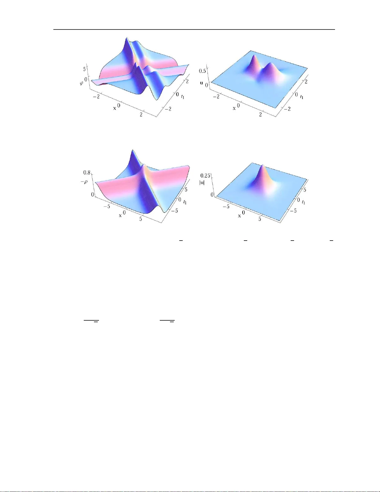
Symmetry , Integrabilit y and Geometry: Metho ds and Applications SIGMA 5 (2009), 002, 18 pages Multicomp onen t Burgers and KP Hierarc hies, and Solutio ns from a Matrix Linear System ⋆ Aristo phanes DIMAKIS † and F o lkert M ¨ ULLER-HOISSE N ‡ † Dep artment of Financial and M anagement Engine ering, University of the A e ge an, 31 F ostini Str., GR-82100 Chios, Gr e e c e E-mail: dimakis@ae ge an .gr ‡ Max-Planck-Institute for Dynamics and Self-Or ganiza tion, Bunsenstr asse 10, D-37073 G¨ ottingen, Germany E-mail: folkert.muel ler-hoissen@ds.mp g.de Received Nov em ber 01, 2008, in f inal form January 04, 200 9; Published online January 08, 2009 doi:10.38 42/SIGMA.20 09.002 Abstract. Via a Cole–Hopf transformatio n, the m ulticomponent linea r heat hierarch y leads to a multicomponent Burger s hierar ch y . W e sho w in particular that a n y s olution o f the latter also solv es a cor resp onding multicomponent (potential) KP hierar ch y . A gener alization of the Co le–Hopf transformation leads to a mor e general relation betw een the multicompo ne nt linear heat hier arch y and the m ulticomponent KP hiera rch y . F rom this results a construction of exa ct so lutio ns o f the la tter via a matrix linear system. Key wor ds: multicomponent KP hiera rch y; Burger s hierarch y; Co le–Hopf tr ansformatio n; Dav ey–Stew artson equation; Riccati equation; dromion 2000 Mathematics Subje ct Classific ation: 37K10 ; 35Q53 1 In tro duction The well- kno wn Cole–Hopf transformation φ = ψ x ψ − 1 translates the nonlinear Bu rgers equatio n in to the linear heat equation [1, 2 , 3]. This extends to a corresp ond ing r elation b et ween the Burgers hierarc h y and the linear heat hierarc h y , and moreo v er to their matrix generalizatio ns. The Cole–Hopf transformation also generates s olutions of the KP hierarch y from (inv ertible) solutions of the linear h eat h ierarc h y [4, 5, 6], and th is extends to the corresp onding matrix hierarc hies [7, 8, 9]. T h ere is also a generalization of the Cole–Hopf trans formation that pr o duces a solution of the (scalar or matrix) KP hierarch y from two solutions of the matrix linear h eat hierarc h y , connected b y an additional relation [7, 8]. F urthermore, th is includ es a constru ction of (matrix) KP solutions from a matrix linear s ystem (see also [10, 11]), w hic h may b e regarded as a f in ite-dimensional v ersion of the Sato theory [12, 13]. In this w ork we extend these results to the m ulticomp onent case. Adm ittedly , this is not a ve ry dif f icult task, on the basis of our previous r esu lts [7 , 11]. W e also tak e this opp ortun it y , ho wev er, to presen t these results in a concise form and to add some relev ant remarks and examples. The usual m u lticomp onen t KP (mcKP) hierarc h y con tains subhierarc hies th at generalize the matrix KP hierarch y by mo d if y in g it with some constan t mat rix B dif ferent from the iden tit y matrix. W e are particularly in terested in suc h matrix hierarchies d if ferent from the ordinary matrix KP hierarc h y . The Da v ey–Stewa rtson equation [14, 15], a tw o-dimen s ional nonlinear Sc hr¨ odinger equation that app eared as a shallo w-w ater limit of the Benney–Roske s ⋆ This pap er is a contribution to the Pro ceedings of the X VI Ith International Colloquium on Integra ble Sy s- tems and Qu antum Symmetries (June 19–22, 2008, Prague, Czech Republic). The full collection is av ailable at http://w ww.emis.de/j ournals/SIGMA/ISQS2008.html 2 A. Dimakis and F. M ¨ uller-Ho issen equation [16, 17], emerges from such a mo dif ied matrix hierarch y (see Section 3 ). It is of course w ell-kno wn to arise from the t w o-component KP hierarc h y . Section 2 recalls the Cole–Hopf transform ation for a multic omp onent Bur gers (mcBurgers) hierarc h y and Section 3 rev eals relations b etw een the m cBurgers and th e mcKP hierarc h y . Sec- tion 4 presen ts the ab o v emen tio ned kin d of generaliza tion of the Cole–Hopf transf ormation whic h determines solutions of the m cKP hierarc h y . F rom this d er ives a fairly simple metho d to con- struct mcKP solutions. This is the sub j ect of Section 5, whic h also pr esents s ome examples. All th is is closely related to a multico mp onent ve rsion of a matrix Riccati h ierarc h y , as brief ly explained in Section 6. Section 7 con tains some conclusions. In the follo wing, let A b e an associativ e (and t ypically noncommutati v e) algebra o v er the complex (or real) num b ers, with identit y elemen t I and su pplied with a stru cture that allo ws to def ine d eriv ativ es w ith resp ect to real v ariables. Let B b e a f inite set of mutually c ommuting elemen ts of A . Although this assump tion is s u f f icien t to establish the results in th is w ork, fur ther assumptions should b e placed on B in particular in order to diminish r edundancy , see the remark at the end of Section 2. With eac h B ∈ B w e asso cia te a sequence of (real or complex) v aria bles t B = ( t B , 1 , . . . , t B ,n , . . . ). F u rthermore, for a fun ction f of { t B } B ∈B w e d ef ine a Miwa shift with resp ect to B ∈ B b y f [ λ ] B ( . . . , t B , . . . ) = f ( . . . , t B + [ λ ] , . . . ), where [ λ ] = ( λ, λ/ 2 , λ/ 3 , . . . ) and λ is an indeterminate. f t n denotes the partial deriv ativ e of f with resp ect to the v ariable t n . 2 Cole–Hopf t ransformation for a m ulticomp onen t Bu rgers h ierarc hy Let us consider the multic omp onent linear h eat h ierarc h y ψ t B,n = B n ∂ n ( ψ ) ∀ B ∈ B , n = 1 , 2 , . . . , (2.1) where ∂ = ∂ x is the op erator of p artial d if ferenti ation with resp ect to a v ariable x , and ψ h as v alues in A . Since ψ t B, 1 = B ψ x , this imp lies the ordinary linear h eat hierarch y ψ t B,n = ∂ n t B, 1 ( ψ ). An y t w o f lows (2.1) comm ute as a consequence of our assu mptions for B (the elemen ts do n ot dep end on { t B } B ∈B and comm ute with eac h other). A functional representa tion 1 of (2.1) is giv en b y λ − 1 ( ψ − ψ − [ λ ] B ) = B ψ x ∀ B ∈ B . (2.2) Prop osition 1. If ψ i s an inve rtible solution of the ab ove multic omp onent line ar he at hier ar chy, then φ = ψ x ψ − 1 (2.3) solves the multic o mp onent Bur gers (mcBur gers) hier ar chy asso ciate d with B , given by the func- tional r epr esentation Ω B ( φ, λ ) = 0 ∀ B ∈ B , (2.4) wher e Ω B ( φ, λ ) := λ − 1 ( φ − φ − [ λ ] B ) − ( B φ − φ − [ λ ] B B ) φ − B φ x . (2.5) 1 W e use this (not quite satisfa ctory) term for an equation that generates a sequen ce of equations b y expansion in p ow ers of an indeterminate. Multicomp onen t Burgers and KP Hierarc hies 3 Pro of . W e ha v e to consider the follo wing system, ψ x = φψ , ψ − [ λ ] B = ( I − λB φ ) ψ ∀ B ∈ B . The int egrabilit y condition ( ψ x ) − [ λ ] B = ( ψ − [ λ ] B ) x yields (2.4). The further in tegrabilit y condi- tion ( ψ − [ λ ] B 1 ) − [ µ ] B 2 = ( ψ − [ µ ] B 2 ) − [ λ ] B 1 is B 2  λ − 1 ( φ − φ − [ λ ] B 1 ) + φ − [ λ ] B 1 B 1 φ  = B 1  µ − 1 ( φ − φ − [ µ ] B 2 ) + φ − [ µ ] B 2 B 2 φ  , whic h is satisf ied as a consequen ce of (2.4) and [ B 1 , B 2 ] = 0.  (2.3) is a Cole–Hopf transformation. The f irst equation that results from (2.4) is φ t B, 1 = B φ x + [ B , φ ] φ, whic h has b een called C -inte gr able N - wave e quation in [9]. If B = I , this r educes to t I , 1 = x . But it is a n ontrivial nonlinear equation if φ do es not comm ute w ith B . The next equation that results from (2.4) is the (noncomm utativ e) Burgers equation φ t B, 2 = φ t B, 1 t B, 1 + 2 φ t B, 1 B φ. Remark 1. In order to a v oid redun dancy and to m aximally extend th e hierarchies, further conditions ha v e to b e imp osed on B . In particular, the elemen ts of B should b e linearly indep en- den t, s ince linear com binations corresp ond to linear com binations of hierarc h y equations. But since pro du cts of elemen ts of B also generate (ind ep endent or redund an t) comm uting f lo ws, the problem is more subtle. If th e algebra is semisimp le, it admits a maximal set of commuting m u- tually annihilating id emp oten ts E a , a = 1 , . . . , N , hence E a E b = δ a,b E a for all a, b = 1 , . . . , N . Then B = { E a } N k =1 is an optimal choic e. In fact, in the follo wing w e do not really address those cases of (non-semisimp le) algebras wh ere s u c h a c hoice do es n ot exist. Rather it turn s out that some more f lexibility in the c hoice of B can b e used to obtain certain in tegrable systems w ithin this framew ork in a more direct w a y , see Section 3. 3 Multicomp onent KP a nd relati ons with the m ulticomp onen t Burgers hierarc h y F or B ∈ B let E B ( λ ) := I − λ ( ω B ( λ ) + B ∂ ) . The “discrete” zero curv at ure condition E B 1 ( λ ) − [ µ ] B 2 E B 2 ( µ ) = E B 2 ( µ ) − [ λ ] B 1 E B 1 ( λ ) (3.1) then leads to the t w o equations λ − 1 ( ω B 2 ( µ ) − ω B 2 ( µ ) − [ λ ] B 1 ) + ω B 2 ( µ ) − [ λ ] B 1 ω B 1 ( λ ) + B 2 ω B 1 ( λ ) x = µ − 1 ( ω B 1 ( λ ) − ω B 1 ( λ ) − [ µ ] B 2 ) + ω B 1 ( λ ) − [ µ ] B 2 ω B 2 ( µ ) + B 1 ω B 2 ( µ ) x and B 2 ω B 1 ( λ ) − ω B 1 ( λ ) − [ µ ] B 2 B 2 = B 1 ω B 2 ( µ ) − ω B 2 ( µ ) − [ λ ] B 1 B 1 . The last equation is solv ed b y ω B ( λ ) = B φ − φ − [ λ ] B B , 4 A. Dimakis and F. M ¨ uller-Ho issen and the f irst equ ation can then b e written in terms of (2.5) as B 2 Ω B 1 ( φ, λ ) − Ω B 1 ( φ, λ ) − [ µ ] B 2 B 2 = B 1 Ω B 2 ( φ, µ ) − Ω B 2 ( φ, µ ) − [ λ ] B 1 B 1 ∀ B 1 , B 2 ∈ B . (3.2) W e take this as our d ef inin g equations of the (more precisely , p otential ) multic omp onent KP (mcKP) hier ar c hy asso ciated w ith B . 2 Remark 2. Cho osing B 1 = B 2 = B in (3.2) and summin g the resulting equation three times with cyclicall y p er muted indeterminates, leads to 3 X i,j,k =1 ǫ ij k  λ − 1 i ( φ − φ − [ λ i ] B ) + φ − [ λ i ] B B φ  − [ λ j ] B B = 0 , whic h is a sp ecial case of the functional form of the mcKP hierarch y in [27]. Let us tak e a closer lo ok at (3.2) with B 1 = B 2 = B . Its λ -indep end en t part is B Ω B ( φ, 0) − Ω B ( φ, 0) − [ µ ] B B = [ B , Ω B ( φ, µ )] , where Ω B ( φ, 0) = φ t B, 1 − [ B , φ ] φ − B φ x . T o f irst order in µ th is giv es B φ t B, 1 x B − 1 2 { B , φ t B, 1 t B, 1 } + 1 2 [ B , φ t B, 2 ] = B φ t B, 1 [ B , φ ] − [ B , φ ] φ t B, 1 B . (3.3) (3.2) is the in tegrabilit y cond ition of Ω B ( φ, λ ) = B θ − θ − [ λ ] B B ∀ B ∈ B , (3.4) with a n ew dep enden t v ariable θ . (3.4 ) represents the mcKP hierarc hy in terms of two dep endent v ariables. By comparison with (2.4 ), this has th e form of an inhomo gene ous mcBurgers hierarc h y . The follo wing is an immediate consequence 3 . Prop osition 2. Any solution of the mcBu r gers hier ar chy also solves the mcKP hier ar c hy. Pro of . (3.4) b ecomes (2.4) if θ = 0.  The representat ion (3.4 ) of the mcKP h ierarc h y has the adv an ta ge that eac h equation only in v olv es a single elemen t from the set B . T o order λ 0 , (3.4 ) yields φ t B, 1 − B φ x − [ B , φ ] φ = [ B , θ ] . (3.5) If B = I , then (3.5) reduces to φ t B, 1 = φ x . Otherwise this is a n on-trivial n on lin ear equation. Subtracting (3.5) from (3.4), leads to λ − 1 ( φ − φ − [ λ ] B ) − φ t B, 1 − ( φ − φ − [ λ ] B ) B φ = ( θ − θ − [ λ ] B ) B . (3.6) The t w o equations (3.5) and (3.6) are equiv alent to (3.4). (3.6) do es not in v olv e deriv ativ es with resp ect to x . F or f ixed B ∈ B , it r ep resen ts the KP hierarch y in A [7], with pro du ct mo dif ied b y B . 2 See also e.g . [18, 19, 20, 21, 22, 6 , 23, 24, 25, 26, 27 ] for dif ferent fo rmulati ons of such a m ulticomponent KP hierarc hy . W e should also mention that the conditions imp osed on the set B can b e relaxed while keeping the hierarc hy p rop erty , see [26] for example. 3 It was f irst noted in [4] th at any solution of the f irst tw o equations of the (scalar) Burgers hierarc h y also solves the (scalar p otentia l) KP equation. In [28, 29] the (f irst tw o) Burgers hierarch y equ ations hav e b een recov ered via a symmetry constraint fro m the KP hierarch y and its linear system. Multicomp onen t Burgers and KP Hierarc hies 5 Prop osition 3. F or any B ∈ B , as a c onse quenc e of the mcKP hier ar chy (3.4) , B φ and also φB solves the or dinary (nonc omm utative) KP hier ar chy. Pro of . This is an immediate consequence of (3.6).  T o f irst order in λ − 1 , (3.6 ) yields 1 2 ( φ t B, 2 − φ t B, 1 t B, 1 ) − φ t B, 1 B φ = θ t B, 1 B . Dif ferentia ting (3.5) w ith resp ect to t B , 1 , and multiplying it by B from the righ t, we can u se the last equation to eliminate θ . In this wa y we reco v er (3.3). As shown in Example 2 b elo w, (3.3) generalizes th e Davey–Stewartson (DS) equation [16, 14, 15, 17]. Eliminating θ from (3.6) b y use of (3.5) th us leads to a (generalized) DS hierarc h y . Example 1. L et B = σ , w here σ 2 = I . Decomp osing φ as φ = D + U, where D := 1 2 ( φ + σ φσ ) , U := 1 2 ( φ − σ φσ ) , (3.3) splits int o the t w o equations 4 D t 1 σ − D x − 2 U 2 = 0 , (3.7) U t 2 σ + U xt 1 + 2 { U, D t 1 } = 0 , (3.8) where w e write t 1 , t 2 instead of t B , 1 and t B , 2 . Let no w A b e the algebra of 2 × 2 matrices ov er C , and σ = diag (1 , − 1). Th en D and U are d iagonal and of f -d iagonal parts of φ , resp ectiv ely . W riting U =  0 u v 0  , hence u := φ 1 , 2 , v := φ 2 , 1 , (3.9) and in tro ducing s := tr( φ ) = φ 1 , 1 + φ 2 , 2 , r := φ 1 , 1 − φ 2 , 2 , w e obtain the system u t 2 − u xt 1 − 2 us t 1 = 0 , v t 2 + v xt 1 + 2 v s t 1 = 0 , (3.10) and s t 1 = r x , s x = r t 1 − 4 uv . The in tegrabilit y conditions of the latter t w o equations are s t 1 t 1 − s xx = 4( uv ) x , r t 1 t 1 − r xx = 4( uv ) t 1 . (3.11) The t w o equations (3.10) together with the f irs t of (3.11) constitute a fairly simple system of thr ee nonlinear coupled equations, where all v ariables can b e taken to b e real. Allo wing complex dep enden t and indep enden t v ariables, after a complex transformation the system for the dep endent v ariables u , v , s can b e f urther reduced to the DS equ ation, see the next example. Of course, the ab o v e system (3.1 0) and (3.11) can also b e deriv ed from the u sual t w o-c omp onent KP hierarc h y (see e.g. [27]), and the transformation to DS is we ll-kno wn. Setting v = 0, we obtain from (3.10) and (3.11) the follo wing line ar equations 5 , u t 2 − u xt 1 − 2 ϕu = 0 , ϕ t 1 t 1 − ϕ xx = 0 , (3.12) where ϕ := s t 1 = tr( φ ) t 1 . Th is is probably the simplest system that p ossesses dr omion s olutions, as observ ed in Example 3 in Section 5. 4 A constan t (with resp ect to t 1 ) of integratio n has b een set to zero in order to obtain (3.7). The latter equation can b e obtained more directly as the diagonal part of (3.5). 5 If u d oes n ot dep end on t 2 , then the f irst equ ation is part of a Lax pair for the Nizhnik –No viko v–V eselo v equation. 6 A. Dimakis and F. M ¨ uller-Ho issen Example 2. W e cont in ue with the p revious example an d p erform a transformation to the DS equation by f ir st allo wing the dep enden t v ariables to liv e in a non commutativ e algebra. In this w a y w e obtain a certain n oncomm utativ e generalizatio n of the DS equation (see also [30, 31] for matrix DS v ersions). In terms of F = D t 1 + β U 2 , with β ∈ C , (3.7) b ecomes F t 1 σ − F x = − β ( U 2 ) x + ( U 2 ) t 1 (2 + β σ ) . Dif ferentia ting this with resp ect to x and with r esp ect to t 1 , resp ectiv ely , and eliminating mixed deriv ative s of F f r om the r esulting t w o equ ations, yields F t 1 t 1 − F xx = − β ( U 2 ) xx + 2( U 2 ) xt 1 + ( U 2 ) t 1 t 1 (2 σ + β ) . (3.13) F urtherm ore, (3.8) takes the form U t 2 σ + U xt 1 = − 2 { U, F } + 4 β U 3 . (3.14) Let n ow A b e the algebra of 2 × 2 matrices o ver some unital asso ciativ e alge bra with unit d enoted b y 1, and σ = diag(1 , − 1). Using (3.9 ) and writing F = diag ( f , g ) , (3.13) and (3.14) result in the follo wing equations, u t 2 − u xt 1 = 2( f u + ug ) − 4 β uv u, v t 2 + v xt 1 = − 2( gv + v f ) + 4 β v uv, f t 1 t 1 − f xx = − β ( uv ) xx + 2( uv ) xt 1 + (2 + β )( uv ) t 1 t 1 , g t 1 t 1 − g xx = − β ( vu ) xx + 2( v u ) xt 1 − (2 − β )( v u ) t 1 t 1 . In terms of the new v ariables y = 1 + i κ √ 2 ( x + i t 1 ) , z = 1 − i √ 2 ( x − i t 1 ) , (3.15) with a constan t κ 6 = 0, and w ith the c hoice β = i , this b ecomes u t 2 + u z z + 1 κ 2 u y y = 2( f u + ug ) − 4i uv u, − v t 2 + v z z + 1 κ 2 v y y = 2( gv + v f ) + 4i vuv , f z z − 1 κ 2 f y y = (1 + 2i )( uv ) z z − 1 κ 2 ( uv ) y y − 2i κ ( uv ) y z , g z z − 1 κ 2 g y y = ( − 1 + 2i )( vu ) z z + 1 κ 2 ( v u ) y y + 2i κ ( v u ) y z . (3.16) If the dep en den t v ariables tak e their v alues in a c ommuta tive alge bra, then we obtain u t 2 + u z z + 1 κ 2 u y y = 2 ρu − 4i u 2 v , − v t 2 + v z z + 1 κ 2 v y y = 2 ρv + 4i v 2 u, ρ z z − 1 κ 2 ρ y y = 4i ( uv ) z z , Multicomp onen t Burgers and KP Hierarc hies 7 where ρ := f + g = ϕ + 2i uv (3.17) (with ϕ = tr( φ ) t 1 ). Setting t 2 = − i t and v = i ǫ ¯ u with ǫ = ± 1 and the complex conjugate ¯ u of u , one reco v er s the DS sys tem i u t + u z z + 1 κ 2 u y y = 2 ρu + 4 ǫ | u | 2 u, ρ z z − 1 κ 2 ρ y y = − 4 ǫ ( | u | 2 ) z z , (3.18) where now y , z , t , κ 2 , ρ are tak en to b e r eal. Clearly , this system is more quic kly obtained from (3. 10) and (3.1 1) by app lication of the transformation of indep endent v ariables giv en b y (3.15) and t 2 = − i t , and the trans formation (3.17) of d ep endent v ariables. Bu t on our wa y w e obtained the s ystem (3.16) whic h (with t 2 = − i t ) ma y b e of interest as a non commutativ e v ersion of the DS equation (see [30, 31] for alternativ es). W e conclude that the DS equation (and a corresp onding hierarc h y) is obtained from a matrix KP h ierarc h y , but the latter has to b e generalized by in tro duction of a matrix B dif ferent from the unit matrix. Of course, this hierarc h y is em b edded in the usual t w o-c omp onent KP hierarc h y . 3.1 The asso ciated Sato–Wilson system and its translation in to a Burgers hierarch y (3.1) is the in tegrabilit y cond ition of the linear system ˜ ψ − [ λ ] B = E B ( λ ) ˜ ψ ∀ B ∈ B . If W is an in v ertible solution of E B ( λ ) W = W − [ λ ] B E 0 ,B ( λ ) , E 0 ,B ( λ ) := I − λB ∂ , (3.19) then the linear system is mapp ed to ψ − [ λ ] B = E 0 ,B ( λ ) ψ where ψ := W − 1 ˜ ψ . The latter is the linear heat hierarc h y (2.2). The ansatz W = I + X n ≥ 1 w n ∂ − n , inserted in to the functional form (3.19) of the Sato–Wilson equations, leads to λ − 1 ( w n − w n, − [ λ ] B ) − B w n,x − ( B φ − φ − [ λ ] B B ) w n = B w n +1 − w n +1 , − [ λ ] B B , (3.20) where n = 0 , 1 , . . . and w 0 = I . F rom the n = 0 equation w e get w 1 = − φ . In terms of θ := − w 2 , the n = 1 equation turn s out to b e the f unctional form (3.4) of the mcKP hierarch y . Let u s in tro duce Φ := Λ ⊺ + e 1 ( φ, − w 2 , − w 3 , . . . ) , (3.21) where e ⊺ 1 = ( I , 0 , . . . ), and Λ :=    0 I 0 0 · · · 0 0 I 0 · · · . . . . . . . . . . . . . . .    (3.22) 8 A. Dimakis and F. M ¨ u ller-Hoissen is the shift op erator matrix with transp ose Λ ⊺ . Then (3.20) can b e expressed as the f ollo w ing mcBurgers hierarc h y , Ω B (Φ , λ ) ≡ λ − 1 (Φ − Φ − [ λ ] B ) − ( B Φ − Φ − [ λ ] B B )Φ − B Φ x = 0 ∀ B ∈ B . (3.23) The linear system of the mcKP hierarc h y has th us b een reform ulated as an mcBurgers hierarc hy with an inf inite matrix v ariable of a sp eci al form. W e note that (3.21) has th e form of a c omp anion ma trix , a blo c k of a F r ob enius normal form matrix. This m ak es cont act with r ecen t wo rk in [9], wh ere seve ral integ rable systems were reco v er ed from equations of a Burgers hierarc h y with dep en den t v ariable of F rob enius n ormal form. All these systems are kno wn to arise as reductions of the mcKP hierarch y . As a consequence of (3.23 ) w ith Φ of the form (3.21 ), it f ollo w s that φ = e ⊺ 1 Φ e 1 solv es the mcKP hierarc h y in A . In the follo wing section, w e shall see that Φ of the form (3.21) results, as a particular case, from a quite general result ab out solutions of a somewhat generalized mcKP hierarch y . 4 Generalization of the Cole –Hopf transformation W e generalize (3.4) to Ω B ,Q (Φ , λ ) = B Θ − Θ − [ λ ] B B ∀ B ∈ B , (4.1) where Ω B ,Q (Φ , λ ) := λ − 1 (Φ − Φ − [ λ ] B ) − ( B Φ − Φ − [ λ ] B B ) Q Φ − B Φ x , (4.2) with a constant ob ject Q . W e assume that the co nstituen ts are elemen ts of linear sp aces and that the pr o ducts are def ined . (4. 1) d etermines a generalization of the mcKP hierarc h y , sin ce non- linear terms now in v olv e Q (which mo dif ies the pro duct). The follo wing generalizes a theorem in [7] (see also [8]). Theorem 1. L et X , Y b e solutions of the multic omp onent line ar he at hier ar c hy, i.e. λ − 1 ( X − X − [ λ ] B ) = B X x , λ − 1 ( Y − Y − [ λ ] B ) = B Y x , (4.3) for al l B ∈ B , and furthermor e X x = RX + QY , (4.4) with c onstant obje cts R , Q . If X is invertible and if al l B ∈ B c ommute with R , then Φ = Y X − 1 (4.5) solves the mcKP Q hier ar chy (4.1) with Θ = Φ R . Pro of . Using (4.5) in the def inition (4.2), we ha v e Ω B ,Q (Φ , λ ) = ( B Φ − Φ − [ λ ] B B )( X x − QY ) X − 1 + ( λ − 1 ( Y − Y − [ λ ] B ) − B Y x ) X − 1 − Φ − [ λ ] B ( λ − 1 ( X − X − [ λ ] B ) − B X x ) X − 1 , whic h reduces to Ω B ,Q (Φ , λ ) = ( B Φ − Φ − [ λ ] B B ) R as a consequence of (4 .3) and (4. 4). Since [ B , R ] = 0, this take s the form (4.1 ) w ith Θ = Φ R .  Multicomp onen t Burgers and KP Hierarc hies 9 No w we set u p the stag e for applications of the th eorem. Let A ( M , N ) := Mat( M × N , C ) ⊗ A , where Mat ( M × N , C ) is the space of complex M × N matrices. Let Φ, Θ, Y t ak e v alues in A ( M , N ), and X in A ( N , N ). F urtherm ore, let Q ∈ A ( N , M ) and R ∈ A ( N , N ) comm ute with all B ∈ B . If Q has r an k one over A , in the sense that Q = V U ⊺ with constant ve ctors U , V , with en tries in A , and if U and V co mm ute with all B ∈ B , then φ = U ⊺ Φ V solv es the mcKP hierarc h y in A , pro vided that Φ solv es (4.1). In th is w a y , an y solution X , Y of th e linear equations formulate d in the ab o v e theorem generates an A -v alued solution φ of th e mcKP hierarc h y (3.2). Cho osing M = N , (4.5) is a Cole–Hopf transformation if Y = X x . Th en (4.4) b ecomes ( I − Q ) X x = R X . Let e k denote the N -comp onen t v ector w ith all en tries zero except for the iden tit y elemen t in the k th row. a) S etting Q = e N e ⊺ N and R = N − 1 P k =1 e k e ⊺ k +1 (whic h is the left shift op erator: R e k = e k − 1 , k = 2 , . . . , N , an d R e 1 = 0), one f inds that (4.4) restricts X to the form of a Wr onski matrix (see also [8]), X =      X (1) X (2) · · · X ( N ) ∂ ( X (1) ) ∂ ( X (2) ) · · · ∂ ( X ( N ) ) . . . . . . . . . . . . ∂ N − 1 ( X (1) ) ∂ N − 1 ( X (2) ) · · · ∂ N − 1 ( X ( N ) )      . X (1) , X (2) , . . . , X ( N ) are in dep end en t functions with v alues in A . Th e remaining assump tion (4.3) in the theorem requires them to b e solutions of the multico mp onent h eat hierarc h y . b) Let R = Λ ⊺ with the inf inite shift op er ator matrix (3.22), and Q = e 1 e ⊺ 1 . Then (4.4) says that X has to b e a pseudo-Wr onski matrix X =      X (1) X (2) X (3) · · · ∂ − 1 X (1) ∂ − 1 X (2) ∂ − 1 X (3) · · · ∂ − 2 X (1) ∂ − 2 X (2) ∂ − 2 X (3) · · · . . . . . . . . . . . .      , (4.6) where ∂ − 1 is the formal inv erse of ∂ . This structure app eared in [9] (equations (14) and (50) therein). (4.3) demands that X (1) , X (2) , . . . solv e the multicomponent heat hierarc h y . With (4.6), Φ = X x X − 1 has the form (3.21) and hence determines a solution of (3.23). 5 Solutions of the m ulticomp onen t KP hierarc h y from a matrix linea r system In order to derive some classes of mcKP solutions via theorem 1 more explici tly , in the framework sp ecif ied in S ection 4 (after the theorem) w e extend (4.4) to Z x = H Z , (5.1) where Z =  X Y  , H =  R Q S L  , with new constan t ob jects L ∈ A ( M , M ) and S ∈ A ( M , N ) that comm ute with all B ∈ B . The t w o equations (4.3) then com bine to λ − 1 ( Z − Z − [ λ ] B ) = B Z x ∀ B ∈ B . 10 A. Dimakis and F. M ¨ u ller-Hoissen T aking (5.1) into account, th is is equiv alen t to Z t B,n = ( B H ) n Z ∀ B ∈ B , n = 1 , 2 , . . . . (5.2) Note th at B and H commute as a consequence of our assump tions. With a suitable choic e of the algebra A , the solution of the matrix linear system (5.1), (5.2) is giv en by Z ( x, t ) = e ξ ( x, t ; H ,B ) Z 0 , (5.3) where ξ ( x, t ; H, B ) := xH + X B ∈B ∞ X n =1 t B ,n ( H B ) n , and t stands for { t B } B ∈B . De comp osing Z int o X and Y , theorem 1 implies that Φ = Y X − 1 solv es the mcKP Q hierarc h y (4.1). F urtherm ore, if rank( Q ) = 1 o v er A , h ence Q = V U ⊺ with constan t v ectors U and V , then the A -v alued v ariable φ = U ⊺ Φ V solv es the corresp ondin g mcKP h ierarc h y . The exp onen tial in (5.3 ) can b e computed explicitl y if additional assumptions are made concerning the form of H (see [11], in particular). T hen Φ is obtained v ia (4.5 ). Case 1. Let S = 0 an d Q = RK − K L (5.4) with a constan t N × M matrix K (o v er A ) that commutes with all B ∈ B . Then we obtain Φ = e ξ ( x, t ; L, B ) C e − ξ ( x, t ; R, B )  I N − K e ξ ( x, t ; L, B ) C e − ξ ( x, t ; R, B )  − 1 , (5.5) where I N is the N × N u nit matrix ov er A (so that the diagonal entries are the id entit y I in A ), and C is an arbitrary constan t M × N matrix (with entries in A ). Φ solv es the mcKP Q hierarc h y (asso ciated with B ), with Q given by (5.4). 6 If moreov er Q = V U ⊺ with vec tors U , V that comm ute with all B ∈ B , th en φ = U ⊺ Φ V solv es the mcKP hierarc h y in A . Of course, it remains to solv e the rank one condition (o v er A ) RK − K L = V U ⊺ . (5.6) If M = N and if C is inv ertible, then (5.5) s implif ies to Φ =  e ξ ( x, t ; R, B ) C − 1 e − ξ ( x, t ; L, B ) − K  − 1 , whic h remains a solution if w e r eplace C − 1 b y an arbitrary constant N × N matrix ˜ C (with en tries in A ). Example 3. C ho osing the comp onen ts of the matrices L , R as L ij = p i δ ij I , R k l = q k δ k l I , (5.7) 6 In particular, if M = N and Q = I N , then Φ (with K , L , R solving RK − K L = I N ) is a solution of the N × N matrix (ov er A ) mcKP hierarc h y . Multicomp onen t Burgers and KP Hierarc hies 11 with constan ts p i , q k , (5.6) is solv ed by K k j = 1 q k − p j u k v j , (5.8) where u k and v j are th e comp onen ts of U and V , r esp ectiv ely . W e elab orate one of the simp lest cases in some detail. Let us c ho ose A as the algebra of 2 × 2 matrices o v er C , L = pI 2 , R = q I 2 , with constan ts p and q , Q = I = I 2 , and B = { B } w ith B = diag (1 , − 1) (motiv ated b y the examples in Section 3). Then we hav e ξ ( x, t ; L, B ) = d iag( ξ + ( x, t ; p ) , ξ − ( x, t ; p )) with ξ ± ( x, t ; p ) := px + ∞ X n =1 p 2 n t 2 n ± ∞ X n =0 p 2 n +1 t 2 n +1 (5.9) (writing t n instead of t B ,n ), and ξ ( x, t ; R, B ) is obtained by exc hanging p by q in these expres- sions. W riting C =  c 1 c 2 c 3 c 4  (5.10) with constan ts c i , w e obtain (with U = V = I 2 ) 7 φ ( x, t ) = 1 D ( x, t )  c 1 e ξ + ( x, t ; p ) − ξ + ( x, t ; q ) + f ( x, t ) c 2 e ξ + ( x, t ; p ) − ξ − ( x, t ; q ) c 3 e ξ − ( x, t ; p ) − ξ + ( x, t ; q ) c 4 e ξ − ( x, t ; p ) − ξ − ( x, t ; q ) + f ( x, t )  , (5.11) where f ( x, t ) := c 1 c 4 − c 2 c 3 p − q e ξ + ( x, t ; p )+ ξ − ( x, t ; p ) − ξ + ( x, t ; q ) − ξ − ( x, t ; q ) , D ( x, t ) := 1 + 1 p − q  c 1 e ξ + ( x, t ; p ) − ξ + ( x, t ; q ) + c 4 e ξ − ( x, t ; p ) − ξ − ( x, t ; q ) + f ( x, t )  . This is a solution of (3.3), with B = diag (1 , − 1), and its hierarc h y , and its comp onents thus pro vide us with the solution u = c 2 D e ξ + ( x, t ; p ) − ξ − ( x, t ; q ) , v = c 3 D e ξ − ( x, t ; p ) − ξ + ( x, t ; q ) , s = 1 D  c 1 e ξ + ( x, t ; p ) − ξ + ( x, t ; q ) + c 4 e ξ − ( x, t ; p ) − ξ − ( x, t ; q ) + 2 f  (5.12) of th e sy s tem (3.10), (3.11). φ is r e gular (for all t ) in particular if all constant s are real, c 1 c 4 > c 2 c 3 , and either p > q , c 1 > 0, c 4 > 0, or p < q , c 1 < 0, c 4 < 0. Fig. 1 presen ts a dromion 8 solution within this family . If c 3 = 0, we hav e v = 0 and (5.12) determines a solution of th e line ar equations (3.12). 9 An extrem um of u for a regular solution then mo v es (in “time” t 2 ) with constan t amplitude along the curve giv en by x = − ( p + q ) t 2 − 1 2( p − q ) log  c 1 c 4 ( p − q ) 2  , t 1 = 1 p − q log  − p q r c 4 c 1  . The last expression sho ws that, for a dromion solution, p and q must h a v e opp osite signs. 7 Since ξ ± ( x, t ; p ) − ξ ± ( x, t ; q ) = ( p − q )( x ± t 1 ) + ( p 2 − q 2 ) t 2 + · · · , this solution b ecomes indep endent of t 2 (i.e. “static”) if p = − q . 8 The characteristic features of a dromion are its exponential lo calization and th at it is accompanied by a f ield structure of intersecting line solitons. See [32, 33, 34, 35, 36, 37, 38, 39, 40 , 41 ] for the Dav ey–Stew artson case, and esp ecially [42] for an illuminating structu ral analysis and t h e app earance of dromions as solutions of other equations. 9 In this case, D factorizes, D = „ 1 + c 1 p − q e ξ + ( x, t ; p ) − ξ + ( x, t ; q ) « „ 1 + c 4 p − q e ξ − ( x, t ; p ) − ξ − ( x, t ; q ) « . 12 A. Dimakis and F. M ¨ u ller-Hoissen Figure 1. A dromion solution o f (3.10) a nd (3.11) at t 2 = 0, g iven by (5.12) with p = 2, q = − 1, c 1 = c 4 = 1, c 2 = 1 / 2 and c 3 = 0. The left plot shows ϕ = s t 1 = tr( φ ) t 1 . As a consequence of c 3 = 0, we hav e v = 0. Hence this is a ctually a s o lution of the line ar equations (3.12) and ϕ so lves the linear w av e equation. Regarding t 1 as a n evolution parameter , the plot of ϕ shows t wo colliding humps (with amplitudes having opp os ite sig ns) that annihilate at t 1 = 0. With 0 6 = c 3 < 2, the plots r emain qualitatively the sa me as long as c 3 is suf f iciently far b elow the upper b ound, and v attains a shap e similar to that o f u . Figure 2. Solutions of (3.1 0) and (3 .11) at t 2 = 0, g iven b y (5.11) with p = 2, c 1 = c 4 = 1, c 2 = c 3 = 1 / 2. The f irst tw o plots, wher e q = 0, show kinks (see (5.13)). In the last tw o plots, where q = − 1 / 5, these bec ome exp onentially lo caliz e d structure s . F or q = 0 in (5.12), setting t n = 0 for n > 2, w e ha v e u = c 2 p 2  c 1 p + c 4 pe − 2 pt 1 + e − pt 1 ( p 2 e − p ( x + pt 2 ) + ( c 1 c 4 − c 2 c 3 ) e p ( x + pt 2 )  − 1 , v = c 3 p 2  c 4 p + c 1 pe 2 pt 1 + e pt 1 ( p 2 e − p ( x + pt 2 ) + ( c 1 c 4 − c 2 c 3 ) e p ( x + pt 2 )  − 1 . (5.13) If c 1 c 4 > c 2 c 3 and c 1 p > 0, c 4 p > 0 (or c 1 c 4 < c 2 c 3 and c 1 p < 0, c 4 p < 0), these functions ob viously r epresen t w edge-shap ed k in ks in the xt 1 -plane, see also Fig. 2. Cho osing p > 0 and switc hing on a negativ e q , these wedges b ecome lo ca lized and , arou n d certain negativ e v alues of q , then tak e the dr omion form. Fig. 3 sho ws plots of a t w o-dromion solution d etermined b y (5.7) with L = diag(3 I 2 , 2 I 2 ), R = diag( − 2 I 2 , − (3 / 2) I 2 ), and 10 C =     1 1 2 0 0 0 1 0 0 0 0 2 1 0 0 5 3     . The d iagonal 2 × 2 b lo c ks of these matrices co rresp ond to matrix d ata of single dromions. Suc h a sup erp osition is obtained f or any t w o solutions, p ro vided that of f-diagonal b lo c ks of the 10 If all lo w er-diagonal entries of C are zero, we obtain v = 0 and th us a so lution of the linear equations (3.12). The plots are surprisingly insensitive with resp ect t o changes in this range of parameters, as long as the of f- diagonal entries in a diagonal blo ck are not all close to zero an d th e determinant of the blo ck is not close to zero. Multicomp onen t Burgers and KP Hierarc hies 13 Figure 3. A t wo-dromion solutio n o f (3.10) and (3.11) at t 2 = 1 , determined by the data sp ecif ied in Example 3. The le ft plot s hows ϕ = s t 1 = tr( φ ) t 1 . Figure 4. A dromion solution o f the Dav ey–Stewartson-I equation with ǫ = − 1 at t 2 = 0, see the end of Example 3. Here w e c hose p 1 = p 2 = (1 + i ) / √ 2, q 1 = − q 2 = (1 − i ) / √ 2, c 1 = − c 2 = i √ 2, c 3 = c 4 = √ 2. Here ρ is given by (3 .17). matrix K exist suc h that (5.6) can b e sati sf ied. T his is so in the restricted case considered ab o v e (see (5.7) and (5.8)), w hic h in particular leads to multi-dromion solutions. In tro ducing non-zero constan ts in the of f-diagonal b lo c ks of C , leads to solutions with more complicated b eha viour. Setting t n = 0, n > 2, the transition to the Da v ey–Ste w artson system (3.18) with κ = 1, whic h is the DS-I case, is giv en b y the transformation of indep enden t v ariables x = 1 + i 2 √ 2 ( z − i y ) , t 1 = − 1 − i 2 √ 2 ( z + i y ) , t 2 = − i t. The dep enden t v ariables are u and ρ , th e latter giv en by (3.17). W e ha v e to tak e the additional constrain t v = i ǫ ¯ u in to accoun t (see Example 2). One reco v ers a DS-I dromion within the class of solutions restricted b y q 1 = ¯ p 1 , q 2 = − ¯ p 2 , c 1 imaginary and c 4 real, and c 3 = ± i ¯ c 2 with sign corresp ondin g to ǫ = ± 1. Fig. 4 shows an example. Case 2. Let M = N , R = L , S = 0, and Q = J + [ L, K ] , (5.14) with constant N × N matrices K and J (o v er A ) that commute with all B ∈ B . F urthermore, J has to commute with L , i.e. [ J, L ] = 0. Then Φ = e ξ ( x, t ; L, B ) C e − ξ ( x, t ; L, B )  I N + ( ξ ′ ( x, t ; L, B ) J − K ) e ξ ( x, t ; L, B ) C e − ξ ( x, t ; L, B )  − 1 , (5.15) where C is an arb itrary constan t N × N matrix (with en tries in A ) and ξ ′ ( x, t ; L, B ) := x + X B ∈B ∞ X n =1 nt B ,n L n − 1 B n . 14 A. Dimakis and F. M ¨ u ller-Hoissen If also Q = V U ⊺ with v ectors U , V that commute with all B ∈ B , th en φ = U ⊺ Φ V solv es the mcKP hierarc h y in A . It remains to solv e J + [ L, K ] = V U ⊺ . (5.16) A natural c hoice for J is th e unit matrix I N , but ther e are others. (5.15) can also b e w ritten as Φ =  e ξ ( x, t ; L, B ) ˜ C e − ξ ( x, t ; L, B ) + ξ ′ ( x, t ; L, B ) J − K  − 1 (5.17) with an arbitrary constant N × N mat rix ˜ C . 11 If ˜ C is c hosen such th at it comm utes w ith L and B , then Φ an d the corresp onding solution φ of the mcKP hierarch y are pur ely r ational functions of the indep enden t v ariables. A lo calized solution of th is kind, hence with r ational deca y , is usually called a “lump”. The follo wing example in particular demonstrates that ther e can b e we ak er conditions that lead to solutions with rational d eca y . Example 4. Ch o osing B = diag(1 , − 1), L = diag( p 1 , p 2 ) and Q = I 2 , (5.1 4) is solv ed by K = diag ( k 1 , k 2 ). Expressing C again as in (5.10), we f in d e ξ ( x, t ; L, B ) C e − ξ ( x, t ; L, B ) =  c 1 c 2 e ξ + ( x, t ; p 1 ) − ξ − ( x, t ; p 2 ) c 3 e − ξ + ( x, t ; p 1 )+ ξ − ( x, t ; p 2 ) c 4  , with ξ ± ( x, t ; p ) def ined in (5.9), and ξ ′ ( x, t ; L, B ) = diag( ξ ′ + ( x, t ; p 1 ) , ξ ′ − ( x, t ; p 2 )), where ξ ′ ± ( x, t ; p ) := x + ∞ X n =1 2 nt 2 n p 2 n − 1 ± ∞ X n =0 (2 n + 1) t 2 n +1 p 2 n . Then (5.15) leads to the follo wing solution of (3.3), with B = diag(1 , − 1), and its h ierarc h y , φ ( x, t ) = 1 D ( x, t )  c 1 + d ( ξ ′ − ( x, t ; p 2 ) − k 2 ) c 2 e ξ + ( x, t ; p 1 ) − ξ − ( x, t ; p 2 ) c 3 e − ξ + ( x, t ; p 1 )+ ξ − ( x, t ; p 2 ) c 4 + d ( ξ ′ + ( x, t ; p 1 ) − k 1 )  , where d := c 1 c 4 − c 2 c 3 and D ( x, t ) := 1 + c 1 ( ξ ′ + ( x, t ; p 1 ) − k 1 ) + c 4 ( ξ ′ − ( x, t ; p 2 ) − k 2 ) + d ( ξ ′ + ( x, t ; p 1 ) − k 1 )( ξ ′ − ( x, t ; p 2 ) − k 2 ) . The comp onents u = φ 1 , 2 and v = φ 2 , 1 , together with s = tr( φ ) = d D  ξ ′ + ( x, t ; p 1 ) + ξ ′ − ( x, t ; p 2 ) + c  , with a constan t c , thus solve the system (3.10), (3.11). F or c 3 = 0, this determin es a solution of the linear equations (3.12). The transition to the Da v ey– Stew artson system (3.18) with κ = i , whic h is the DS-I I case, in v olv es the transformation of indep enden t v ariables x = 1 + i 2 √ 2 ( y + z ) , t 1 = 1 − i 2 √ 2 ( y − z ) , t 2 = − i t. W e set t n = 0, n > 2, in the follo wing. T he lum p s olution of the DS-I I equation [43, 44, 17] (see also [45, 46, 40, 47]) is obtained as follo ws from the ab o ve form ula. Besides taking acco unt of the constrain t v = i ǫ ¯ u , w e ha v e to arrange in particular that the exp onential in u b ecomes a phase 11 In t he transition from (5.15) to (5.17), one assumes that C is invertible with inve rse ˜ C . But ˜ C n eed not b e inv ertible in order that ( 5.17) determines a solution of the mcKP Q hierarc hy . Multicomp onen t Burgers and KP Hierarc hies 15 factor (up to some constant f actor), i.e. the real p art of its exp onen t has to b e constan t. This requires setting p 2 = − i ¯ p 1 . It is more tr ic ky to f in d conditions on the remaining parameters suc h that D 6 = 0 for all y , z , t , so that the solution is regular. C ho osing c 4 = − i ¯ c 1 , c 3 = i ¯ c 2 , k 2 = − i ¯ k 1 , and renaming k 1 , p 1 to k , p , w e f in d th at D = 1 4 ( | c 1 | 2 + 2 | c 2 | 2 )  ( y − y 0 − v y t ) 2 + ( z − z 0 − v z t ) 2  + 2 | c 2 | 2 | c 1 | 2 + 2 | c 2 | 2 , where v y = − 2 Im( p ), v z = 2 Re( p ), and y 0 = Re( k ) − 2 Re( c 1 ) | c 1 | 2 + 2 | c 2 | 2 , z 0 = Im( k ) + 2 Im( c 1 ) | c 1 | 2 + 2 | c 2 | 2 . The resulting DS-I I solution u = c 2 D e i (Im( p ) y +Re ( p ) z − Re( p 2 ) t ) , ρ = 1 4 D 2  ( | c 1 | 2 + 2 | c 2 | 2 ) 2  ( z − z 0 − v z t ) 2 − ( y − y 0 − v y t ) 2  − 8 | c 2 | 2  , with ρ def in ed in (3.17) and ǫ = 1, is regular whenever c 2 6 = 0 and repr o duces a w ell-kno wn lump solution. Again, (l ump) solutions can b e s up erp osed by taking matrix data of (lump) solutions as diagonal blo cks of larger matrices L and C . It then essentia lly remains to determine the of f- diagonal blo c ks of the new matrix K so that (5.16) holds. 6 The matrix Riccati system asso ciated with the m u lticomp onen t KP h ierarc hy W riting H n =:  R n Q n S n L n  , the matrix linear system (5.1), (5.2) implies the matrix Ric c ati system Φ x = S + L Φ − Φ R − Φ Q Φ , (6.1) Φ t B,n = B n S n + B n L n Φ − Φ B n R n − Φ B n Q n Φ . (6.2) The t w o solution f amilies presente d in Section 5 solv e this m atrix Riccati system, with the resp ectiv e conditions imp osed on the matrices L , Q , R , S . Abstracting fr om matrices and thin king of L , R , S as (noncomm utativ e) algebraic ob jects, their elimination from the ab o v e system leads to the mcKP hierarc h y with pro d uct mo d if ied b y Q (cf. [48]). T o some extent the ab o v e Riccati system thus expresses the mcKP hierarc h y as a hierarc h y of ordinary dif feren tial equations. Finite-size matrix Ricc ati equations, in particular with constant co ef f icien t matrices as abov e, w ere discu s sed in a con text r elated to in teg rable systems already long ago (see e.g. [49, 50]), but app aren tly not in the con text of the KP hierarc h y . A sp ecia l in f in ite-size matrix R iccati system inv olving the s h ift op erator in inf inite dimensions app eared, how ever, in the f ramew ork of th e Sato theory (see e.g. [51, 13]). I n the one-comp on ent case with B = I , the ab o v e Riccati system, with su itable conditions imp osed on the co ef f icient m atrices, also generates solutions of the BKP and the CK P hierarc h y [52]. Th e Riccati system indeed generates solutions of v arious in tegrable systems and therefore deserves to b e studied in its o wn right. 16 A. Dimakis and F. M ¨ u ller-Hoissen Remark 3. F or f ixed r ∈ N , r > 1, and for some f ixed B ∈ B , let us consider the condition ( H B ) r Z 0 = Z 0 P , with an N × N matrix P (o v er A ). F or the solution (5.3) of the linear matrix system (5.2), this implies ( H B ) nr Z = Z P n for n ∈ N , hence B nr ( R nr X + Q nr Y ) = X P n and B nr ( S nr X + L nr Y ) = Y P n , and th us the algebraic Riccati equations B nr ( S nr + L nr Φ) = Y P n X − 1 = Φ X P n X − 1 = Φ B nr ( R nr + Q nr Φ). The corresp onding equations (6.2) of the Riccati system then read Φ t B,nr = B nr ( S nr + L nr Φ) − Φ B nr ( R nr − Q nr Φ) = 0 , n = 1 , 2 , . . . . Hence φ solv es the ( r , B )- r e duction , i.e. the r - r e duction (m ulticomp onen t v ersion of r th Gelfand– Dic k ey h ierarc h y) with resp ect to B . 7 Conclusions An y solution of a m ulticomp onent Bur gers (mcBurgers) hierarc h y is a solution of the corre- sp ond ing multico mp onent K P (mcKP) hierarch y . F urthermore, there is a fu nctional equation that determines the mcKP h ierarch y and h as the form of an inhomo gene ous mcBurgers hierar- c h y fun ctional equation. W e h a v e also shown that the mcKP linear system is equiv alen t to a mcBur gers h ierarc h y , where the d ep endent v ariable has the str ucture of an inf in ite F rob enius companion matrix (whic h in particular make s con tact with [9]). Moreo v er, we h a v e shown how solutions of a mcKP hierarch y are obtained f r om solutions of a m ulticomp onen t linear heat hierarc h y via a generalized Cole–Hopf tr an s formation. An imp ortant sub case generates solutions of a mcKP hierarc h y from solutions of a matrix linear system and we pr esented some explicit s olution f ormulae. They comprise in particular Da v ey– Stew artson dromions and lump solutions. There is certainly a lot more to b e (re)disco v ered using the rather simp le but quite general metho d in Section 5 to construct exact solutions, but we are far from a systematic w a y to explore th e pr op erties of solutions obtained in this wa y . F urthermore, w e hav e stressed the role of a m atrix Riccati hierarc h y in this con text. References [1] Hopf E., The partial dif feren tial equation u t + uu x = µu xx , Comm. Pur e Appl. Math. 3 (1950), 201–230. [2] Cole J.D., On a qu asi-linear parabolic equation occurring in aero dyn amics, Quart. Appl. Math. 9 (1951), 225–236 . [3] Sa w ada K., Kotera T., A meth o d for f inding N -soliton solutions of the K.d.V. eq u ation and K.d.V.-like equation, Pr o gr. The or et. Phys. 51 (1974), 1355–1367. [4] Mikhailo v A., Shabat A ., Sokolo v V., The symmetry approach to classif ication of integrable eq uations, in What Is Integrabilit y?, Editor V. Zak haro v, Springer Ser. Nonline ar Dynam. , Sprin ger, Berlin, 1991, 115–184 . [5] Guil F., Ma˜ nas M., ´ Alv arez G., The Hopf–Cole transformation and the KP equation, Phys. L ett. A 190 (1994), 49–52. [6] Guil F., Ma ˜ nas M., The Dirac equation and integrable systems of KP typ e, J. Phys. A: Math. Gen. 29 (1996), 641–665 . [7] Dimakis A., M¨ uller-Hoissen F., Burgers and KP hierarchies: a fun ctional represen tation approach, T he or et. and M ath. Phys. 152 (2007), 933–947, nlin.SI/0610045. [8] Dimakis A., M¨ uller-Hoissen F., With a Cole–Hopf transformation to solutions of the noncommutative KP hierarc hy in terms of W ronski matrices, J. Phys. A: Math. The or. 40 (2007), F321–F329, nlin.SI/0701052. Multicomp onen t Burgers and KP Hierarc hies 17 [9] Zenc huk A.I., San tini P .M., The remark able relatio ns among PD Es integ rable b y the inv erse sp ectral trans- form metho d, by the metho d of characteristi cs and by the H opf–Cole transformation, J. Phys. A: Math. The or. 41 (2008), 185109, 28 pages, arXiv:0801.3945 . [10] Dimakis A., M¨ uller-Hoissen F., Nonasso ciativit y an d integrable hierarchies , nlin.SI/0601001 . [11] Dimakis A ., M ¨ uller-Hoissen F., W eakly nonassociative algebras , Riccati and KP h ierarc hies, in Generalized Lie Theory in Mathematics, Physics and Beyond, Editors S. Silvestro v, E. P aal, V. Abramov an d A. S tolin, Springer, Berlin, 2008, 9–27, nlin.SI/0701010 . [12] Sato M., Sato Y., Soliton equ ations as dynamical systems on inf inite dimensional Grassmann manifold, in Nonlinear P artial Dif ferentia l Equations in A pplied Science, Editors H. F ujita , P .D. Lax and G. Strang, North-Hol land M ath. Stud. , V ol . 81, North-H olland, Amsterdam, 1982 , 259–271 . [13] T ak asaki K., Geometry of u niversal Grassmann manifold from algebraic p oint of v iew, R ev. Math. Phys. 1 (1989), 1–46. [14] Da ve y A ., Stewa rtson K., On three-dimensional pack ets of surface w a ves, Pr o c. R oy. So c. L ondon Ser. A 338 (1974), 101–11 0. [15] Anker D., F reeman N.C., On t he soliton solutions of the D a vey–Stew artson equation for long wa ves , Pr o c. R oy. So c. L ondon Ser. A 360 (1978), 529–540. [16] Benney D., Rosk es G., W a ve instabilities, Stud. Appl. Math. 48 (1969), 377–385. [17] Nak amura A., General superp osition of solitons and vari ous ri pplons of a t w o-dimensional nonlinear Schr¨ odinger equation, J. Math. Phys. 23 (1982), 1422–142 6. [18] Sato M., Soliton equations as dy n amical sy stems on inf inite dimensional Grassmann manif olds, in Random Systems and Dynamical Systems (Kyoto, 1981 ), RIM S Kokyur oku 439 (1981), 30–46. [19] Date E., Jimbo M., Kashiw ara M., Miw a T., T ransformation groups for soliton equations. I I I. Op erator approac h to the Kadomtsev–P etviash vili equation, J. Phys. So c. Jap an 50 (1981), 3806–3812 . [20] Ka jiw ara K., Matsukidaira J., S atsuma J., Conserved quantities of tw o-component K P hierach y , Phys. L et t. B 146 (1990), 115–118. [21] Oev el W., Darb oux theorems and Wronskian form ulas for integ rable systems. I. Constrained KP f lows, Phys. A 195 (1993), 533–576 . [22] Bergv elt M.J., ten Kro od e A.P .E., Partitions, vertex op erator constructions and multi-component KP equ a- tions, Pacific J. Math. 171 (1995), 23–88, hep-th/9212087. [23] Doliw a A., Ma ˜ nas M., Martinez Alonso L., Medina E., S antini P .M., Charged free fermions, vertex op erators and the cla ssical theory of conjugate nets, J. Phys. A : Math. Gen. 32 (1999 ), 1197–1216, solv-int/98030 15 . [24] Dic k ey L., Soliton equations and Hamiltonian systems, 2nd ed., A dvan c e d Series in Mathematic al Physics , V ol. 26, W orld Scientif ic Publishing Co., Inc., River Edge, N J, 2003. [25] Kac V.G., v an der Leur J.W., The n -comp onent KP hierarch y and representation theory , J. M ath. Phys. 44 (2003), 3245–32 93, hep- th/9308137. [26] Kundu A., Strampp W., Deriv ative and higher-order ext en sions of Da v ey–Stewartso n equ ation from matrix Kadomtse v–Petviash vili hierarc hy , J. M ath. Phys. 36 (1995), 4192–42 02, hep-th /9311153. [27] Bogdano v L.V., K onop elc henko B.G., Analytic-b ilinear approac h to in tegrable hierarc hies. I I. Multicomp o- nent K P and 2D T o da lattice hierarc hies, J. Math. Phys. 39 (1998), 4701–47 28, solv-int/96090 09 . [28] Cheng Y ., Li Y.S., Constraints of the 2 + 1 dimensional integrable soliton systems, J. Phys. A: Math. Gen. 25 (1992), 419–431 . [29] Konopelchenko B., Strampp W., N ew reductions of th e K adomts ev–Petvias hvili and t w o-dimensional T o da lattice hierarchies v ia symmetry constrain ts, J. Math. Phys. 33 (1992), 3676–3686 . [30] Y uro v A., B¨ ac klund–Schlesinger transformations for Da vey–Stew artson equations, The or et. and Math. Phys. 109 (1996), 1508–1 514. [31] Lezno v A.N., Y uzbashya n E.A., Multi-soliton solutions of the tw o-dimensional matrix Davey–Stew artso n equation, Nucle ar Phys. B 496 (1997), 643–653, hep - th/9612107. [32] Boiti M., Leon J.-P ., Martina L., P empinelli F., Scattering of lo calized solitons in the plane, Phys. L ett. A 132 (1988), 432–43 9. [33] F ok as A.S., San tini P .M., Coherent structures in m ultidimensions, Phys. R ev. L et t. 63 (1989), 1329–1333. [34] San tini P .M., Energy ex change of interacting coherent structu res in multidimensio ns, Phys. D 41 (1990), 26–54. 18 A. Dimakis and F. M ¨ u ller-Hoissen [35] Hietarin ta J., Hirota R ., Multidromion solutions t o t he Dav ey–Stew artson equation, Phys. L et t. A 145 (1990), 237–244 . [36] Jaulen t M., Manna M., Ma rtinez-Alonso L., F ermionic analysis of Dav ey–Stew artson dromions, Phys. L ett. A 151 (1990), 303–307 . [37] Nak ao T., W adati M., Da vey–Stew artson equation and prop erties of dromion, J. Phys. So c. Jap an 62 (1993), 933–947 . [38] Sall’ M.A., The Da vey–Stew artso n equations, J. Math. Sci. 68 (1994), 265–270. [39] Gils on C.R., Nimmo J. J.C., A direct metho d for dromion sol utions of the Davey–Stew artson equations and their asymptotic prop erties, Pr o c. R oy. So c. L ondon Ser. A 435 (1991), 339–357. [40] P elino vsky D., On a struct u re of the explicit solutions to the Dav ey–Stew artson equations, Phys. D 87 (1995), 115–122 . [41] Guil F., Ma˜ nas M., Deformation of the dromion and solitof f solutions of the Dav ey–Stew artson I equation, Phys. L et t. A 209 (1995), 39–47. [42] Hietarin ta J., One-dromion solutions for generic classes of equations, Phys. L ett. A 149 (1990), 113–118. [43] Satsuma J., Ablo witz M.J., Tw o-dimensional lumps in n onlinear disp ersive systems, J. M ath. Phys. 20 (1979), 1496–15 03. [44] Nak amura A., Explo de-d eca y mo de lump solitons of a tw o- dimensional nonlinear Schr¨ odinger eq uation, Phys. L et t. A 88 (1982), 55–56. [45] F ok as A.S., Ablow itz M.J., Method of solution for a class of m ultidimensional nonlinear evol ution equations, Phys. R ev. L ett. 51 (1983), 7–10. [46] Ark adiev V., Pogrebk o v A ., Poli v ano v M., Inverse scattering tran sform metho d and soliton solutions for Dav ey–Stew artson II equ ation, Phys. D 36 (1989), 189–197. [47] Ma˜ nas M., Santini P .M., Solutions of the Da vey–Stew artson I I equation with arbitrary rational lo calization and nontrivial interaction, Phys. L ett . A 227 (1997), 325–334. [48] Dimakis A ., M¨ uller-Hoissen F., A new approac h to deformation equations of noncomm utative KP hierarc hies, J. Phys. A: Math. The or. 40 (2007), 7573–75 96, math-p h/0703067. [49] Win ternitz P ., Lie groups and solutions of n onlinear partial dif ferential equations, in Nonlinear Phenomena (Oaxtep ec, 1982), L e ctur e Notes in Phys. , V ol. 189, S p ringer, Berlin, 1983 , 263–331 . [50] del Olmo M.A., R o driguez M., Winternitz P ., Sup erp osition form ulas for rectangular matrix R iccati equ a- tions, J. Math. Phys. 28 (1987), 530–535. [51] Dorfmeis ter J., N eher E., Szmigielski J., A utomorphisms of Banach manifolds asso ciated with t he KP- equation, Quart. J. M ath. Oxf or d Ser. (2) 40 (1989), 161–195. [52] Dimakis A., M¨ uller-Hoissen F., BKP and CKP revisited: The o dd KP system,