Robust Cognitive Beamforming With Partial Channel State Information

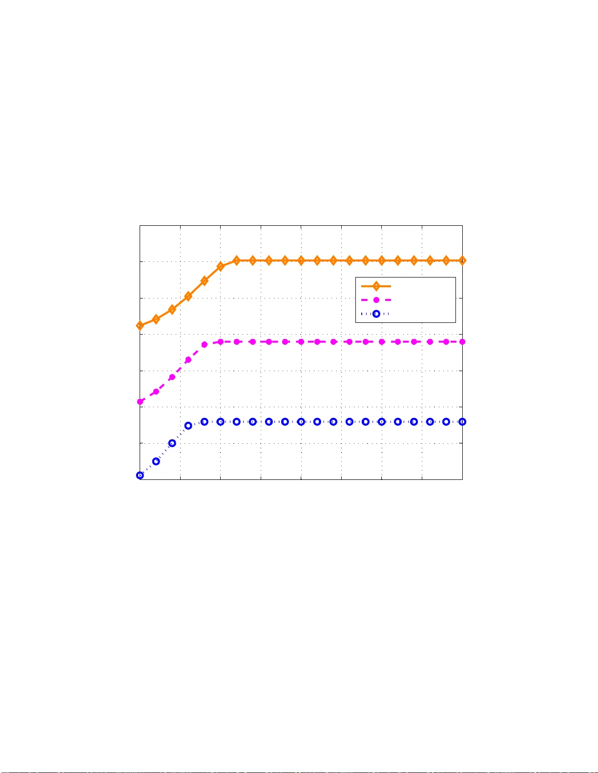
IEEE TRANSA CTIONS ON WIRELESS COMMUNICA TIONS (REVISED) Rob ust Cogniti v e Beamforming W ith Pa rtial Channel S tate Information ⋆ Lan Zhang † , Y ing-Chang Liang ‡ , Y an Xin † , and H. V incent Poor ∗ Suggested Editorial Areas: Cognitive radio, Multiple-inp ut si ngle-output (MISO), Partial channel state information , Po wer allocation, W ireless netw orks. ⋆ The work is supp orted by the National Uni versity of S ingapore (NUS) und er Grants R-263-000-314-101 , R -263-000-3 14-112, and R-263-000-47 8-112, by a NUS Research Scholarship, and by the U.S. Nati onal Science Foundation under Grants ANI-03-38807 and CNS-06-25637. This work was done while Y . Xin was visiting Princeton Univ ersity . † L. Zhang and Y . Xin are with the Department of E lectrical and Computer Engineering, National Univ ersi ty of Singapore, Singapore 118622 . (email: zhanglan@nus.edu .sg; elexy@nus.edu .sg) ‡ Y .-C. Liang is with Institute of Info comm Research, A*ST AR, 21 Heng Mui K eng T errace, Singapore 11961 3. (email: ycliang@i2r .a- star .edu.sg) ∗ H. V . Poor is with the Dep artment of Electrical Engineering, Princeton Uni versity , Princeton, NJ 08544, USA, (email: poor@princeton.ed u). October 24, 2018 DRAFT IEEE TRANSA CTIONS ON WIRELESS COMMUNICA TIONS (REVISED) 1 Abstract This pap er co nsiders a spectrum sharing ba sed cog nitive radio (CR) co mmun ication system, which consists of a seconda ry u ser (SU) having multiple transmit antenn as and a single recei ve antenna an d a primar y u ser (PU) h aving a single recei ve an tenna. The channel state information (CSI) on the link of the SU is assumed to be per fectly known at the SU transmitter (SU-Tx ). Howe ver, due to loose c oopera tion between the SU and the PU, on ly p artial CSI of the link b etween the SU-Tx and the PU is av ailable at th e SU-Tx . W ith the partial CSI and a prescrib ed tran smit power con straint, o ur de sign o bjective is to determ ine the transmit sign al covariance matrix that max imizes the rate of the SU while keeping the interferen ce power to the PU below a thresh old for all the p ossible ch annel realization within an un certainty set. This problem , termed the ro bust cognitive beamforming problem , can be naturally formu lated as a semi-infinite pr ogramm ing (SIP) prob lem with infinitely many constraints. T his problem is first transforme d into th e seco nd or der con e p rogram ming (SOCP) problem and then solved v ia a standa rd interior po int algorithm . Then, an analytical solution with much reduc ed complexity is developed fro m a geometric p erspective. It is shown that both algorithms ob tain the same o ptimal solution. Simulation examples are presented to validate the effectiveness of the prop osed algo rithms. Keywords : Cognitiv e ra dio, inter ference c onstraint, m ultiple-inp ut single-o utput (MISO), partial chan nel state informa tion, power allocation, rate maximization . I . I N T RO D U C T I O N One of the fundamental challenges faced by the wireless communi cation industry is how to meet rapidly g rowing demands for wi reless services and appl ications with limited radio spectrum. Cognitive radio (C R) technology has been propo sed as a promising solution to tackle such a challenge [1]–[8]. In a spectrum sharing b ased CR network, the secondary u sers (SUs) are allowed to coexist with the primary user (PU), subject to th e con straint, namely t he interference constraint, t hat the interference power from t he SU to the PU i s less than an acceptable value. Ev idently , the purpose of the imposed interference constrain t is to ensu re that the quality of service (QoS) of the PU is not degraded due to the SUs. T o b e aware of wheth er the i nterference constraint is satisfied, the SUs needs obtain knowledge of the radio en vironment cognitively . In this paper , we consid er a spectrum sharing based CR comm unication scenario, i n whi ch the SU uses a multiple-inpu t single-outpu t (MISO) channel and the primary user (PU) h as one receive antenna. October 24, 2018 DRAFT IEEE TRANSA CTIONS ON WIRELESS COMMUNICA TIONS (REVISED) 2 W e assu me th at the channel state information (CSI) about the SU link is perfectly known at the SU transmitter (SU-Tx). Howev er , owing to loos e coop eration between the SU and the PU, only the mean and cova riance of the channel between the SU-Tx and th e PU is av ailable at t he SU-Tx. W ith this CSI, our design ob jectiv e is, for a given t ransmit power constraint, to determine the transmit si gnal cov ariance matrix t hat m aximizes the rate of the SU whil e keeping the interference power to th e PU below a thresho ld for all the po ssible channel realizations wit hin an uncertainty s et. W e t erm thi s desig n problem the robust cognitiv e beamform ing design problem. In non-CR settings, the study of m ultiple antenna systems with partial CSI has received consi derable attention in the past [9], [10]. Specifically , the paper [10] considers t he case in which the recei ver has perfect CSI but th e t ransmitter has only partial CSI (mean feedback or covariance feedback). It was proved in [10] that the optimal transm ission directions are the same as t hose of the eigen vectors o f the channel covariance matrix. Howe ver , t he optim al power allocation solut ion was not given in an analytical form. A universal opt imality conditi on for beamform ing was explored in [11], and quantized feedback was studied in [12]. In CR settings, power allocation st rategies ha ve been developed for multipl e access channels (MA C) [13] and for point -to-point multiple-inpu t multiple-output (MIMO) channels [14 ]. Particularly , the solution developed in [14] can be viewed as cognitive beamforming since th e SU-Tx forms its main beam direction wi th aw areness of its i nterference to the PU. A closed-form method has b een present in [14]. A water -fill ing based algorithm is proposed in [13] to obtain the suboptim al po wer allocation strategy . Ho wever , the papers [13] and [14] assume that perfect CSI about the link from the SU-Tx to the PU is av ai lable at the SU-Tx. Due t o loose cooperation between the SU and the PU, it could be diffic ult or even infeasibl e for the SU-Tx to acquire accurate CSI between the SU-Tx to the PU. In this paper , we formu late the robust cognitive beamformi ng design problem as a semi-i nfinite programming (SIP) p roblem, which is d iffi cult to solve directly . The contribution of thi s paper can be summarized as follows. 1) Se veral important properties of the optimal solution of the SIP problem, t he rank-1 property , and the s uffi cient and necessary conditions of the op timal s olution, are presented. These properti es would transform the SIP problem in to a finite constraint optim ization problem. October 24, 2018 DRAFT IEEE TRANSA CTIONS ON WIRELESS COMMUNICA TIONS (REVISED) 3 2) Based on these properties, we show that t he SIP problem can be transformed into a second order cone p rogramming (SOCP) p roblem, which can be so lved vi a a st andard interior point algorithm. 3) By exploit ing the geometric properties of t he opti mal soluti on, a closed-form soluti on for the SIP problem is also provided. The rest of this p aper is organized as follows. Section II describes the SU MISO commun ication system model, and t he problem formulation of the robust cognitive b eamforming design. Section III presents seve ral important lemm as t hat are used t o dev elop the algorithms . T wo different algorit hms, the SOCP b ased solut ion and the analytical s olution, are de veloped i n Section V and Se ction IV, respectiv ely . Section VI presents si mulation examples, and finally , Section VII concludes t he paper . The following notation is used in th is p aper . Bol dface upp er and lower case lett ers are us ed to denote matrices and vectors, respecti vely , ( · ) H and ( · ) T denote the conjugate transpose and transpose, respectiv ely , I denot es an identity matrix, tr ( · ) denotes the trace operation, and Rank ( A ) denotes the rank of the matrix A . I I . S I G N A L M O D E L A N D P RO B L E M F O R M U L A T I O N W ith reference to Fig. 1, we consider a poi nt-to-point SU M ISO com munication system , where the SU has N transmit antennas and a single receive antenna. The sig nal model of t he SU can be represented as y = h H s x + n , where y and x are the received and transmit ted signals respectively , h s denotes t he N × 1 channel respons e from th e SU-Tx to th e SU-Rx, and n is independ ent and identically d istributed (i.i.d.) Gaussi an noise with zero m ean and unit var iance 1 . Suppos e that the PU has one recei ve ant enna. The channel respo nse from the SU-Tx to the PU is denot ed by an N × 1 vector h . Further , assume that the SU-Tx has perfect CSI for its own link, i.e., h s is perfectly known at the SU-Tx. Ho wever , due to the loose cooperation between t he SU and the PU, only partial CSI about h i s assumed to be av ailable at the SU-Tx. W e assum e that h 0 and R are the mean and covariance 1 Since the SU receiv er cannot differentiate the interference from the PU from the background noise, the term n can be viewed as t he summation of the i nterference and the noise. T he va riance of n does not infl uence the algorithms discussed lat er . Moreov er , the v ariance of n can be measured at the SU receiv er [13]. October 24, 2018 DRAFT IEEE TRANSA CTIONS ON WIRELESS COMMUNICA TIONS (REVISED) 4 of h , respective ly 2 . In previous w ork [10], [15]–[1 7], partial CSI has been consi dered in two extreme cases in a non-CR sett ing. One i s the m ean feedback case, R = σ 2 I , where σ 2 can be vi ewe d as th e var iance of the estim ation error; and the other is the covariance feedback case, where h 0 is a zero vector . In this paper , we study the case where th e SU-Tx knows both the m ean and cov ariance of h in a CR settin g. The obj ectiv e of this paper is t o determ ine t he optimal transmit signal cova riance m atrix s uch that the information rate o f the SU lin k is maximized while the Qo S of the PU is guaranteed under a robust design scenario, i .e., t he instantaneous interference power for the PU s hould remain below a given threshold for all the h i n the uncertain region. Mathematicall y , the problem is formulated as fol lows: Rob ust design problem ( P1 ) : max S ≥ 0 log(1 + h H s S h s ) subject to : tr ( S ) ≤ ¯ P , and h H S h ≤ P t for ( h − h 0 ) H R − 1 ( h − h 0 ) ≤ ǫ, (1) where S is the transm it signal covariance matrix, ¯ P i s the transmit power budget, P t is the interference threshold of the PU, and ǫ is a positive constant. The parameter ǫ characterizes the un certainty of h at the SU. According t o the definiti on of the uncertainty in [18], P1 belongs to a t ype of ellipsoid uncertainty problem, i.e., the uncertain p arameter h is confined in a range of an el lipsoid H , where H : { h | ( h − h 0 ) H R − 1 ( h − h 0 ) ≤ ǫ } . Thus, t he opti mal s olution of problem P 1 can guarantee the interference power const raint of the PU for all the h ∈ H , and thus the robustness of P1 is in th e worst case s ense [19], i.e., in the worst case chann el realization, the interference const raint should also be satisfied. If th e primary transmis sion does not exist, then the interference constraint is excluded, and thus the problem reduces to a trivial beamforming problem. Hence, we on ly focus on the case where the both PU and SU transmissio n exist. Remark 1: An imp ortant observation is that t he objective function in problem P1 remains in var iant when h s undergoes an arbitrary phase rotation. W ithout loss of generality , we assum e, in the sequel, that h s and h 0 hav e the same phase, i.e., Im { h H s h 0 } = 0 . 2 Due to the cogniti ve property , we assume that the SU can obtain the pilot signal from the PU, and thus can detect the channel information from the PU to t he SU. Moreov er , since the SU shares the same spectrum with the PU, based on the channel from the PU to the SU, the statistics of the channel from the SU to the PU can be obtained [15]. Therefore, we can assume that h 0 and R are kno wn to the SU. October 24, 2018 DRAFT IEEE TRANSA CTIONS ON WIRELESS COMMUNICA TIONS (REVISED) 5 Since prob lem P1 has a finite nu mber of decisio n variable S , and is subjected to an infinite nu mber of constraints with respect to the com pact set H , prob lem P1 is an SIP problem [20]. One obvious approach for an SIP probl em is to transform it into a finite const raint problem. Howe ver , there is no univ ersal algo rithm to determine the equiv alent finite constraints such t hat the transformed problem has the same solution as the orig inal SIP problem. In th e following section, we first study sev eral i mportant properties of problem P 1 , which would be used to transform th e SIP problem in to its equiva lent finite constraint counterpart. I I I . P R O P E R T I E S O F T H E O P T I M A L S O L U T I O N The maximi zation p roblem P1 is a con vex opt imization prob lem, and thus h as a uniq ue optim al solution. The following lemm a presents a key property of th e o ptimal solution of probl em P1 (see Appendix A for th e proof). Lemma 1: The optimal covariance matrix S for problem P1 i s a rank-1 matrix. Remark 2: Lemma 1 i ndicates that beamforming is the opti mal t ransmission strategy for p roblem P1 , and the o ptimal t ransmit covariance matrix can be expressed as S opt = p opt v opt v H opt , where p opt is the opt imal t ransmit power and v opt is th e o ptimal beamform ing vector with k v opt k = 1 . Therefore, the ultimate objective of problem P1 i s to determine p opt and v opt . According to Lemma 1, a necessary and sufficient condition for t he optimal so lution of prob lem P1 is presented as foll ows (refer to Appendix B for the proof). Lemma 2: A necessary and suf ficient condition f or S opt to be the globally optimal solution of problem P1 is that there exists an h opt such that S opt = arg max S ,p log(1 + h H s S h s ) , subject to : tr ( S ) ≤ p, 0 ≤ p ≤ ¯ P , h H opt S h opt ≤ P t , (2) where h opt = arg max h h H S opt h , for ( h − h 0 ) H R − 1 ( h − h 0 ) ≤ ǫ. (3) Remark 3: The vector h opt is a ke y elem ent for all h : ( h − h 0 ) H R − 1 ( h − h 0 ) ≤ ǫ , in th e sense that, for the opti mal solut ion, the constraint h H opt S h opt ≤ P t dominates th e whole interference constraint s, October 24, 2018 DRAFT IEEE TRANSA CTIONS ON WIRELESS COMMUNICA TIONS (REVISED) 6 i.e., all the other i nterference constraint s are inactive. Thus, if we can determi ne h opt , the SIP problem P1 is transformed into a finite const raint problem (2). It is worth noting that t he problem (2) has the same form as the problem dis cuss in [14], i n which the CSI on the li nk of the SU and the li nk between SU-Tx and PU are perfectly known at t he SU-Tx. Howe ver , unl ike the problem in [14], h opt in (2) is an unknown parameter . In th e foll owing lemma (see Appendi x C for the proof), the optimal beamforming vector v opt is shown to lie in a two-dimensi onal (2-D) space sp anned by h 0 and the pro jection of h s into the null space of h 0 . Define ˆ h = h 0 / k h 0 k and ˆ h ⊥ = h ⊥ / k h ⊥ k , where h ⊥ = h s − ( ˆ h H h s ) ˆ h . Hence, we ha ve h s = a h s ˆ h + b h s ˆ h ⊥ with a h s , b h s ∈ R . Lemma 3: The optimal beamformin g ve ctor v opt is of the form a v ˆ h + b v ˆ h ⊥ with a v , b v ∈ R . Remark 4: According t o Lem ma 3 , we can search for the optimal beamforming vector v opt on t he 2-D space spanned by ˆ h and ˆ h ⊥ , which s implifies the search process signi ficantly . The optimal v opt found in this 2-D space, is also the globally opt imal solut ion of the orig inal prob lem P1 . As d epicted in Fig. 2, problem P1 is transformed into the problem of determining the beamforming vector v opt in the 2-D space and the corresponding power p opt . Combi ning Lemm a 2 and Lem ma 3, it is easy t o conclude that h opt lies in the space spanned by ˆ h and ˆ h ⊥ . I V . S E C O N D O R D E R C O N E P RO G R A M M I N G S O L U T I O N In this section, we solve problem P1 via a standard i nterior po int alg orithm [19], [21], [22]. W e first transform the SIP problem into a finite const raint problem, and further transform i t into a standard SOCP form, which can be sol ved by using a standard s oftware p ackage such as SeDuMi [23]. One key observation is that if max h ∈H ( ǫ ) h H S h ≤ P t , i.e., th e worst case interference constraint of P 1 is satisfied, then the interference constraint of P 1 holds. Combinin g t his observation with Lem ma 1 , problem P1 can be transformed as: Equiv alent problem ( P2 ): max p ≥ 0 , k v k =1 log(1 + p h H s v v H h s ) subject to : p ≤ ¯ P , max h ∈H ( ǫ ) p h H v v H h ≤ P t , (4) October 24, 2018 DRAFT IEEE TRANSA CTIONS ON WIRELESS COMMUNICA TIONS (REVISED) 7 where H ( ǫ ) := { h | h = h 0 + h 1 } . It is clear th at maxi mizing log (1 + p h H s v v H h s ) is equivalent to maximizing | √ p h H s v | . By defining w = √ p v , the objecti ve function can be re writ ten as | h H s w | . Similarly , the interference po wer can be expressed as | h H w | 2 . Thus, problem P2 can be further transformed to max w | h H s w | subject to : k w k ≤ p ¯ P , max h ∈H ( ǫ ) | h H w | ≤ p P t . (5) According to the definition of H ( ǫ ) , we can re write the worst-case constraint in (5) as max h ∈H ( ǫ ) | h H w | = max h 1 ∈H 1 ( ǫ ) | ( h 0 + h 1 ) H w | ≤ p P t , (6) where H 1 ( ǫ ) := { h 1 | h H 1 R − 1 h 1 ≤ ǫ } . By appl ying the triang le inequality and the fact that √ ǫ k Qw k = max | h H 1 w | for h 1 ∈ H 1 ( ǫ ) (refer t o Appendix D for det ails), the i nterference power ca n be t ransformed as follows: | ( h 0 + h 1 ) H w | ≤ | h H 0 w | + | h H 1 w | ≤ | h H 0 w | + √ ǫ k Qw k , (7) where Q = ∆ − 1 / 2 U with ∆ and U bei ng obtai ned by the eigen value decomp osition of R − 1 as R − 1 = U H ∆ U . Moreover , since the arbitrary p hase rotation of w does not change the value of the objective funct ion or the constraint s, according t o Remark 1 and Lemm a 3, we can assume that w , h s , and h 0 hav e the same phase, i.e., Re { w H h s } ≥ 0 , Im { w H h 0 } = 0 , and Im { w H h s } = 0 . (8) Hence, th e interference const raint can be t ransformed int o two second order cone inequaliti es as foll ows √ ǫ k Qw k + h H 0 w ≤ p P t , and √ ǫ k Qw k − h H 0 w ≤ p P t . (9) By com bining (5) , (9), with (8), problem P1 is transformed i nto t he stand ard SOCP problem as follows max w h H s w subject to : k w k ≤ p ¯ P , Im { w H h 0 } = 0 , √ ǫ k Qw k + h H 0 w ≤ p P t , √ ǫ k Qw k − h H 0 w ≤ p P t . (10) Since the par ameters h s and h 0 , and the v ariable w in (10) ha ve complex values, we first con vert them to its corresponding real-v alu ed form i n order to sim plify the sol ution. Define ˜ w := [ Re { w } T , Im { w } T ] T , October 24, 2018 DRAFT IEEE TRANSA CTIONS ON WIRELESS COMMUNICA TIONS (REVISED) 8 ˜ h 0 := [ Re { h 0 } T , Im { h 0 } T ] T , ˜ h s := [ Re { h s } T , Im { h s } T ] T , ˇ h 0 := [ Im { h 0 } T , − Re { h 0 } T ] T , and ˜ Q :=   Re { Q } − Im { Q } Im { Q } Re { Q }   . W e then can re write the standard SOCP problem (10) as max ˜ w ˜ h H s ˜ w subject to : k ˜ w k ≤ p ¯ P , ˇ h H 0 ˜ w = 0 , √ ǫ k ˜ Q ˜ w k + ˜ h H 0 ˜ w ≤ p P t , √ ǫ k ˜ Q ˜ w k − ˜ h H 0 ˜ w ≤ p P t . (11) Problem (11) can be s olved by a standard interior poin t program SeDuMi [23], which has a polyno- mial complexity . In the next section, we d e velop an analytical algorit hm to solve problem P1 , which reduces the complexity of the interior point based algorit hm substanti ally . V . A N A NA L Y T I C A L S O L U T I O N In this section , we present a geometric approach to problem P1 . W e begin by studying a s pecial case, the mean feedback case, i.e., R = σ 2 I . Due t o its special geomet ric structure, the m ean feedback case problem can be solved via a closed-form algorithm . W e next show that problem P1 can b e transformed into an op timization problem simi lar to th e m ean feedback case. Based on the closed-form solut ion deriv ed for the mean feedback case, t he analyti cal solu tion to problem P1 with a general form o f a cov ariance matrix R is presented i n Subsection V -B. A. Mean F eedback Case Based on t he observation in Lemm a 1 and the definiti on of the mean feedback, the special case of problem P1 with mean feedback can be written as follows. Mean feedback problem ( P3 ): max p ≥ 0 , k v k =1 log(1 + p h H s v v H h s ) subject to : p ≤ ¯ P , p h H v v H h ≤ P t , for k h − h 0 k 2 ≤ ǫσ 2 . (12) Problem P3 has two constraints, i.e., t he transm it power constraint and the i nterference const raint. Similar to the idea i n [13], t he two-constraint problem is decoupled into two single-constraint subprob- October 24, 2018 DRAFT IEEE TRANSA CTIONS ON WIRELESS COMMUNICA TIONS (REVISED) 9 lems: Subpr oblem 1 ( SP1 ): max p ≥ 0 , k v k =1 log(1 + p h H s v v H h s ) (13) subject to : p ≤ ¯ P . (14) Subpr oblem 2 ( SP2 ): max p ≥ 0 , k v k =1 log(1 + p h H s v v H h s ) (15) subject to : p h H v v H h ≤ P t , for k h − h 0 k 2 ≤ ǫσ 2 . (16) In the sequel, we present the algorithm to obtain the o ptimal power p opt and the optimal beamformi ng vector v opt for both subprobl ems in subsectio n V -A.1, and describe the relationsh ip between the subproblems and problem P3 in subsection V -A.2. 1) Solution t o subp r oblems: For SP 1 , the optimal power is cons trained by the transmit power constraint, and thu s p opt = ¯ P . Moreover , s ince there does not exist any constraints on the b eamforming direction, i t is obvious th at the opti mal beamforming direction is equ al to h s , i.e., v opt = h s / k h s k . Thus, t he optimal covariance matrix S opt for SP 1 is ¯ P h s h H s / k h s k 2 . In the foll owing, we focus on the solution to SP2 . SP2 has infinitely many interference constrain ts, and thus i s an SIP problem too. By foll owing a similar line of thin king as i n Lemma 2, SP2 can be transformed i nto an equiv al ent problem that has finite constraints (refer to A ppendix E for the proof) as follows. Lemma 4: SP2 and the fol lowing optimizati on problem: max p ≥ 0 , k v k =1 log(1 + p h H s v v H h s ) , subject to : p h H opt v v H h opt ≤ P t , (17) where h opt = h 0 + √ ǫσ v , have the same optimal solution. According to Lemma 4 , prob lem (17) has the same optimal solution as SP2 . Mo reove r , according to Lemma 3, the optimal solution v of problem (17) lies in the plane spanned by ˆ h and ˆ h ⊥ . W e next apply a geom etric approach to search t he optimal solut ion, i.e., by restricting our search space to a 2-D space. As shown in Fig. 3 , assum e that the angle between v and h 0 is β , and the angle between h s and h 0 is α . It is easy to obs erve th at 0 ≤ α ≤ π / 2 3 . Since v lies in a 2-D space, v can be uni quely 3 This follows because if α ≥ π / 2 , we can always replace h s by − h s without affecting the fi nal result, and t he angle between − h s and h 0 is less than π / 2 . October 24, 2018 DRAFT IEEE TRANSA CTIONS ON WIRELESS COMMUNICA TIONS (REVISED) 10 identified by the angle β . Hence, we need only to search for the optimal angle β opt . By e xploiti ng the relationship between p , v , and β , the t wo-v ariable optimizati on problem (17) can be further transformed into an optim ization problem with a single variable β , which can be readily solved. By observing Fig. 3, t he angle between h s and v is β − α , and hence the objecti ve function of (17) can be expressed as max k v k =1 log(1 + p h H s v v H h s ) = max β log  1 + p k h s k 2 cos 2 ( β − α )  . (18) Clearly , t he maximum rate is achieved if the fol lowing function f ( β ) := p k h s k 2 cos 2 ( β − α ) (19) is maximized. Moreover , i t can be proved by contradi ction that the i nterference constrain t is satisfied with equality , i.e., h H opt S h opt = P t . Thus, we have p h H opt v v H h opt = p ( h 0 + √ ǫσ v ) H v v H ( h 0 + √ ǫσ v ) = p  k h 0 k cos β + √ ǫσ  2 = P t . (20) Hence, the interference constraint is transformed into p = P t  k h 0 k cos β + √ ǫσ  2 . (21) By substitu ting (21) into (19), we have f ( β ) = p k h s k 2 cos 2 ( β − α ) = k h s k 2 P t cos 2 ( β − α )  k h 0 k cos( β ) + √ ǫσ  2 . (22) Thus, the opti mal β opt can be expressed as β opt = arg max f ( β ) = arg max k h s k 2 P t cos 2 ( β − α )  k h 0 k cos( β ) + √ ǫσ  2 . (23) The problem of (23) i s a si ngle va riable optim ization probl em. It is easy to observe that the feasible region for β i s [ α , π / 2 ] . According to the s uffi cient and necessary conditio n for the op timal sol ution of an optimization problem, β opt lies either on the border of the region ( α o r π / 2 ) or on the point which satisfies ∂ f ( β ) /∂ β = 0 . Since ∂ f ( β ) ∂ β = 2 k h s k 2 P t cos( β − α )  sin α − sin( β − α ) √ ǫσ / k h 0 k  k h 0 k 2  cos β + √ ǫσ / k h 0 k  3 , (24) October 24, 2018 DRAFT IEEE TRANSA CTIONS ON WIRELESS COMMUNICA TIONS (REVISED) 11 we can obtain a locally op timal solution β 1 = sin − 1  k h 0 k si n α √ ǫσ  + α b y solving t he e quation ∂ f ( β ) /∂ β = 0 . In th e case when k h 0 k sin α √ ǫσ > 1 , f ( β ) is a non -decreasing fun ction. Hence, t he opti mal β is π / 2 , and we define f ( β 1 ) = −∞ for th is case. Therefore, the global ly optimal solution is β opt = arg max( f ( α ) , f ( π / 2) , f ( β 1 )) . (25) The optim al power p opt can be further obtained b y subst ituting β opt into (21). A ccording to t he definition of β and Lemma 3, we h a ve v opt = a v ˆ h + b v ˆ h ⊥ , (26) where a v = cos( β opt ) and b v = sin( β opt ) . In sum mary , SP2 can b e solved by Algorithm 1 as describ ed in T able I. 2) Optimal solution to pr oblem P3 : In the preceding subsection, we presented the optimal solution s for the two subprobl ems. W e now turn our attent ion to the relati onship b etween probl em P3 and the subproblems, and present t he complete algorithm t o sol ve problem P 3 . Since the conv ex optim ization problem P3 has two cons traints, the opt imal solu tion can be classified int o three cases depending on the activ eness of the constraints : 1) o nly t he transmi t power constraint is activ e; 2) o nly the interference const raint is active; and 3) both constraints are activ e. Relying o n this classi fication, the relationship between the solutions of problem P 3 and the t wo sub problems is described as follows (refer to Appendix F for the proof). Lemma 5: If the opt imal solution S 1 of SP1 satisfies t he constraint of SP2 , th en S 1 is th e o ptimal solution of problem P3 . If t he opt imal solut ion S 2 of SP2 satisfies the cons traint o f SP1 , then S 2 is the optimal solution of problem P3 . O therwise, the op timal solu tion of problem P 3 sim ultaneously satisfies the transmit power constraint and h H opt S h opt ≤ P t with equality . Remark 5: T o apply Lemma 5, we need to test whether S 1 and S 2 satisfy both constraint s. The condition that S 1 satisfies the interference cons traint is P int ≤ P t , where P int = max h h H S 1 h , for k h − h 0 k 2 ≤ ǫσ 2 , (27) where P int can be o btained b y the m ethod discuss ed in Ap pendix D. The condition that S 2 satisfies the transmit power cons traint is tr ( S 2 ) ≤ ¯ P . October 24, 2018 DRAFT IEEE TRANSA CTIONS ON WIRELESS COMMUNICA TIONS (REVISED) 12 W e next discuss the method for finding the solution in the case where neither S 1 nor S 2 is the optimal soluti on of problem P3 . Similarly to th e method in t he preceding sub section, we solve this case from a geometric p erspectiv e. Accordin g to Lemma 5, in the case in which neith er S 1 nor S 2 is the feasible solutio n, the optimal cov ariance S opt must satisfy both constraints wit h equality , i .e., p opt = ¯ P , and p opt h H opt v opt v H opt h opt = P t . (28) Combining these two equalities, we have ¯ P  k h 0 k cos( β ) + √ ǫσ  2 = P t . (29) Thus, β opt = arccos  p P t / ¯ P − √ ǫσ k h 0 k  . (30) Based on β opt , we can obtain v opt from (26). W e sum marize the procedure called Algo rithm 2, which solves the case where both constraints are active for problem P3 , i n T abl e II. Furthermore, we are now ready to present the compl ete algorithm, namely Algorithm 3, to solve problem P3 in T able III. In Algori thm 3, we ob tain the optimal solut ions to SP1 and SP 2 and the optim al soluti on t o the case where bot h constraints are active separately . According to Lemm a 5, t he final sol ution obtained in Algorithm 3 is thus t he optimal soluti on of problem P3 . Pr opos ition 1: Al gorithm 3 obtains th e optimal solutio n of prob lem P3 . B. The Analytical Method fo r Pr oblem P1 In the preceding subsection, the mean feedback problem P3 is s olved vi a a closed-form algorithm. Unlike problem P3 , p roblem P1 has a non-identit y-matrix cov ariance feedback. T o exploit the closed- form algori thm, we first transform problem P 1 int o a problem wit h the mean feedback form as follows. Equiv alent problem ( P4 ): max p, ¯ v log(1 + p ¯ h H s ¯ v ¯ v H ¯ h s ) subject to : p k ∆ 1 / 2 ¯ v k 2 ≤ ¯ P , p ¯ h H ¯ v ¯ v H ¯ h ≤ P t , for k ¯ h − ¯ h 0 k 2 ≤ ǫ, (31) where R − 1 := U H ∆ U obtained by eigen-decomposing R − 1 , ¯ h := ∆ 1 / 2 U h , ¯ h 0 := ∆ 1 / 2 U h 0 , ¯ h s := ∆ 1 / 2 U h s , and ¯ v := ∆ − 1 / 2 U v . By substi tuting these definition s into (31), i t can be ob served that the achiev ed rates and constraints of both prob lem P1 and P4 are equivalent. Thus, the optimal solutio n October 24, 2018 DRAFT IEEE TRANSA CTIONS ON WIRELESS COMMUNICA TIONS (REVISED) 13 of P1 can be obtain ed by solving its equi valent problem P4 . Moreover , the optimal bea mforming vector ¯ v opt of problem P 4 can be easily transformed i nto the optimal sol ution v opt for problem P 1 by letting v opt = U H ∆ 1 / 2 ¯ v opt . Note that it i s not necessary that k ¯ v k = 1 in (31). In the preceding subsection, decoupling the m ultiple constraint prob lem into se veral single constraint subproblems facilitates th e analysis and si mplifies the process of sol ving the probl em. For probl em P4 , it can also be d ecoupled into two subproblems as follows. Subpr oblem 3 ( SP3 ): max p, ¯ v log(1 + p ¯ h H s ¯ v ¯ v H ¯ h s ) (32) subject to : p k ∆ 1 / 2 ¯ v k 2 ≤ ¯ P . (33) Subpr oblem 4 ( SP4 ): max p, ¯ v log(1 + p ¯ h H s ¯ v ¯ v H ¯ h s ) (34) subject to : p ¯ h H ¯ v ¯ v H ¯ h ≤ P t for k ¯ h − ¯ h 0 k 2 ≤ ǫ. (35) It is easy to observe that SP3 i s equiv alent to SP1 , and the optim al transmit cov ariance m atrix of SP3 can be obt ained in the same way as that for SP1 . M oreover , SP4 is t he same as SP2 , and thus it can be solved by Algorithm 1 dis cussed in Subsection V -A.1. The relationship between problem P4 and subproblems SP3 and SP4 is si milar to the one between P3 and corresponding subproblems as depi cted in Lemma 5, i.e., if either opt imal solut ion of SP3 or SP4 satisfies both cons traints, t hen it is the globally optimal s olution; otherwise, the opti mal so lution satisfies both constraints wit h equ alities. W e hereafter need to consider only t he case in which the solutions of b oth subproblems are not feasible f or problem P4 . F or this case, the two equal ity constraints can be written as foll ows. k ∆ 1 / 2 ¯ v k = 1 , and max  ¯ h H ¯ v ¯ v H ¯ h  = P t ¯ P , for k ¯ h − ¯ h 0 k 2 ≤ ǫ. (36) Assume that the ang le between ¯ h 0 and ¯ v is ¯ β , and that ¯ p := k ¯ v k . Similar to Lemma 3, the op timal ¯ v lies in a plane sp anned by ˆ ¯ h and ˆ ¯ h ⊥ , where ˆ ¯ h = ¯ h 0 / k ¯ h 0 k , ˆ ¯ h ⊥ = ¯ h ⊥ / k ¯ h ⊥ k , and ¯ h ⊥ = ¯ h s − ( ˆ ¯ h H ¯ h s ) ˆ ¯ h . Thus, if we can determ ine ¯ β and ¯ p from (36), then the op timal ¯ v can be identified by ¯ v = ¯ p  cos( ¯ β ) ˆ ¯ h + sin( ¯ β ) ˆ ¯ h ⊥  . (37) October 24, 2018 DRAFT IEEE TRANSA CTIONS ON WIRELESS COMMUNICA TIONS (REVISED) 14 Based on the new variables ¯ β and ¯ p , th e constraints (36) can be transformed as follows. ¯ p    ∆ 1 / 2  cos( ¯ β ) ˆ ¯ h + sin( ¯ β ) ˆ ¯ h ⊥     = 1 , (38) and , ¯ p  cos( ¯ β ) k ¯ h 0 k + √ ǫ  = r P t ¯ P . (39) According to (38), we ha ve ¯ p = 1    ∆ 1 / 2  cos( ¯ β ) ˆ ¯ h + sin( ¯ β ) ˆ ¯ h ⊥     . (40) Substitutin g (40) i nto (39), we have r P t ¯ P    ∆ 1 / 2  cos( ¯ β ) ˆ ¯ h + sin( ¯ β ) ˆ ¯ h ⊥     = cos( ¯ β ) k ¯ h 0 k + √ ǫ. (41) Hence, the optimal ¯ β can be obtained by solving (41), and ¯ v opt can be obtain ed by substitut ing ¯ β into (37). In summary , the procedure t o sol ve the case in which b oth constraints are active is listed as Algorithm 4 i n T able IV. Mo reove r , we are now ready to present the complete alg orithm, namely Algorithm 5, for so lving problem P1 in T able V. In Algori thm 5, we ob tain the optimal solut ions to SP3 and SP 4 and the optim al soluti on t o the case where b oth constraints are activ e separately . According to Lemma 5 , th e final result obtained in Algorithm 5 is thus th e optimal soluti on of problem P1 . Pr opos ition 2: Al gorithm 5 achiev es the optim al solution of problem P1 . Remark 6: The c omplexity of the interio r poi nt algorithm for the S OCP problem (11) is O ( N 3 . 5 log( 1 ε )) , where ε denotes the error tolerance. For A lgorithm 5, a maxi mum of O (log( 1 ε )) operations is needed to solve (41), and the comp lexity for each operation is O (log ( N 2 )) . Hence, the computati on complexity required for Algorit hm 5 is O ( N 2 log( 1 ε )) , whi ch is much less than that of the interior point algorithm. V I . S I M U L A T I O N S Computer simulations are provided in thi s section to e valuate the performance of the proposed algorithms. In the s imulation s, it is assu med that the entries o f the channel vectors h s and h 0 are modeled as independent circul arly symmetric complex Gauss ian random variables with zero m ean and unit variance. Moreover , we d enote by l 1 the distance between the SU-Tx and the SU-Rx, and by l 2 October 24, 2018 DRAFT IEEE TRANSA CTIONS ON WIRELESS COMMUNICA TIONS (REVISED) 15 the dis tance between the SU-Tx and the PU. It is assumed that the same path loss mo del is used t o describe t he transmissions from the SU-Tx to the SU-Rx and to the PU, and t he path loss e xponent is chosen to be 4 . The noi se power is chosen to be 1 , and the transmit power and interference power are defined in dB relative to t he noise power . For all cases, we choose P t = 0 dB. A. Comparison of the Analyt ical Solution and the Solutio n Obtained by the SOCP Algo rithm In this sim ulation, we com pare the two results obtained by a st andard SOCP algorithm (SeDuMi ) and Algorithm 3. W e consider the sys tem with N = 3 , l 2 /l 1 = 2 , and ¯ P ranging from 3 dB to 10 dB. In Fig. 4, we can see that t he results obtained by different alg orithms coi ncide. This i s because both algorithms determine the optimal solution. Compared with the SOCP algorithm so lution, Algorithm 3 obtains the solution directly , and thus it has lower complexity . In Fig. 5, we com pare the t wo results obtained by SeDuMi and Algorithm 5 . W e consid er the system with N = 3 , ¯ P = 5 dB, and l 2 /l 1 ranging from 1 to 10 . The cov ariance mat rix R is generated b y R H 1 R 1 , where each element o f R 1 follows Gaussian d istribution with zero mean and unit variance. From Fig. 5, we can see that t he results obtained by th e two algo rithms coincide again. M oreover , we note that t he achiev able rate with ǫ = 0 . 2 is always greater than or equal to the rate with ǫ = 0 . 3 , since a l ar ger ǫ corresponds t o the st ricter constraints. B. Effectiveness of the Interfer ence Constraint In this sim ulation, we apply Algorithm 3 to solve problem P3 . In Fig. 6, we depict the achiev able rate versus t he ratio l 2 /l 1 under different transmi t power constraints. The increase of the ratio l 2 /l 1 corresponds th e decrease of the in terference p ower constraint . As shown in Fig. 6, wi th an increase of l 2 /l 1 , the achiev able rate increases due to the lower interference constraint. Unt il the ratio l 2 /l 1 reaches a certain value, the achieva ble rate remains unchanged, since the transm it po wer constraint dominates the result, and the in terference constraint becomes inactive. C. The Activeness of the Const raints In this simu lation, we compare the ac hieve d rates of problem P1 with a single transm it power constraint, a singl e interference constraint and both constraint s. Here, we choose N = 3 , ǫ = 0 . 2 , and October 24, 2018 DRAFT IEEE TRANSA CTIONS ON WIRELESS COMMUNICA TIONS (REVISED) 16 generate R i n the same way as in the first si mulation example. Fig. 7 plots three achie vable rates fo r diffe rent constraints, respective ly . It can be observed from Fig. 7 that the rate under t wo const raints is alwa ys less than or equal to t he rate under a si ngle constraint. Obviously , this is due to th e fact that extra constraints reduce the degree of freedom of the transmit ter . V I I . C O N C L U S I O N S In this paper , the robust cognitive beamformin g desig n problem has been in vestigated, for the SU MISO communication s ystem in which only partial CSI of t he link from the SU-Tx to the PU is a vailable at th e SU-Tx. Th e problem can be formulated as an SIP optimi zation problem. T wo approaches have been proposed to obt ain t he op timal s olution of t he prob lem; one approach is based on a st andard interior point algorithm, while the other approach s olves t he problem analytically . Simulation examples hav e been used to present a comparison of t he two approaches as well as to study the eff ectiv eness and active ness of imposed constraints. This work initiat es research in robust desi gn of cog nitive radios. W e are currently extending these methods t o t he mo re general case with mu ltiple receive antennas and mul tiple PUs. Ot her in teresting extensions include more practical scenarios, such as the case in which the SU channel information is also partially known at the SU-Tx. A P P E N D I X A. Pr oo f o f Lemma 1: Problem P1 i n volves infinitely many constraints. Denote t he set o f active constraints by C , the cardinali ty of the set C by K , and the channel respon se related to t he k th element of the set C by h k . According to the Karush-Kuhn-T ucker (KKT) condit ions for P1 , we have: h s (1 + h H s S h s ) − 1 h H s + Φ = λ I + K X i =1 µ i h i h H i , (42) tr ( Φ S ) = 0 , (43) where Φ is the dual variable associated w ith t he constraint S ≥ 0 , and λ and µ i are the dual variables associated with the transmit powe r constraint and the interference const raint, respectively . First, we October 24, 2018 DRAFT IEEE TRANSA CTIONS ON WIRELESS COMMUNICA TIONS (REVISED) 17 assume that λ 6 = 0 , and thus the rank of the rig ht h and si de of (42 ) is N . Since the first term o n t he left hand side of (42) has rank one, we h a ve Rank ( Φ ) ≥ N − 1 . (44) Moreover , since S ≥ 0 and Φ ≥ 0 , from (43) we hav e tr ( Φ S ) = tr ( U H Λ U S ) = tr ( Λ U S U H ) = tr ( Λ ˜ S ) = 0 , where U H Λ U is the eigen value decompositio n of matrix Φ , and ˜ S := U S U H . By applying eigen value decompositi on to ˜ S , we have ˜ S := P i τ i s i s H i , where τ i is the i th eigen value and s i is the corresponding eigen vector . W e next show Rank ( S ) + Rank ( Φ ) ≤ N by contradiction. Suppose that Rank ( S ) + Rank ( Φ ) > N . Then, there exists an index j such that the j th element of s i and the j th diagonal el ement of Λ are non-zero sim ultaneously . Th us, it is impossi ble that the equation tr ( Λ ˜ S ) = 0 hold s. It follows that Rank ( S ) + Rank ( Φ ) ≤ N . Combining thi s wi th (44), we hav e Rank ( S ) ≤ 1 . Second, we ass ume that λ = 0 in (42). In this case, S m ust l ie in t he space s panned by h i , i = 1 , · · · , K . L et the di mensionalit y of t he space be M . Therefore, we can restrict Rank ( Φ ) ≤ M . Thus, the reminder of th e proof is the same as that of the case λ 6 = 0 , and the proof is com plete.  B. Pr oo f of Lemma 2 : First, we cons ider the suffi ciency p art of this lemma. W e assum e that there exists a covariance matrix S opt and an h opt that satisfy the conditions (2) and (3) si multaneously . Since S opt satisfies both the t ransmit power const raint and the interference constraint, S opt is a feasible solution for problem P1 . Moreover , if we assume t hat there exists another solution S s , which results i n a lar ger achiev able rate for the SU link, then a contradiction will be deriv ed. W ithout loss of generality , we assume t hat the cons traint set, which consists of all the active int erference cons traints for S s , is denoted by T . W e divide the set T into two types: one ty pe i s h opt ∈ T , and the other type is h opt / ∈ T . Assume that C s and C opt are the achie vable rates for the co variance m atrices S s and S opt , respectiv ely . In the case of h opt ∈ T , we ha ve C s ≤ C opt , since C opt is obt ained with fewer constraints. Since problem P1 is a con vex optimizati on probl em that has a unique optim al sol ution, S opt is indeed the opti mal solution. In the case of h opt / ∈ T , we can observe that S opt satisfies the constraints in T , and S s satisfies the constraint h opt . According to the lem ma in [13], this case does not exist. W e next proceed to prove the necessity part. Suppose that S opt is t he opti mal solution of problem October 24, 2018 DRAFT IEEE TRANSA CTIONS ON WIRELESS COMMUNICA TIONS (REVISED) 18 P1 . According to Lemm a 1, we hav e S opt = p opt v opt v H opt . Thus, problem P1 is equiv al ent to max S ≥ 0 log(1 + h H s S h s ) subject to : tr ( S ) ≤ p opt , h H S h ≤ P t , for ( h − h 0 ) H R − 1 ( h − h 0 ) ≤ ǫ. (45) According to Lemma 6, there is a unique h opt = h 0 + r ǫ v H opt Rv opt α Rv opt , (46) which is the op timal sol ution of max h ∈H ( ǫ ) h H S h ≤ P t . Thus , for problem (45), only tr ( S ) ≤ p opt and h H opt S h opt ≤ P t are activ e constraints. Thus, it is obvious that probl em (45) and problem (2) hav e the same optim al solution. Hence, the proof is complet e.  C. Pr oof of Lemma 3 : The proof of Lemma 3 i s divided into two parts. The first part is to prove that v opt is in the form of α v ˆ h + β v ˆ h ⊥ , where α v ∈ C and β v ∈ C . The second part is to prove α v ∈ R and β v ∈ R . In the foll owing proof, we assum e that α k ∈ C are some proper complex scalars. According to Lemma 2, and Th eorem 2 in [14], we have v opt = α 1 h opt + α 2 h s . (47) According to Lemma 6, we hav e h opt = h 0 + α 3 v opt = h 0 + α 3  α 1 h opt + α 2 h s  = h 0 + α 1 α 3 h opt + α 2 α 3 h s . (48) According to (48), it can be observed that h opt can be expressed by the lin ear combination of h 0 and h s , where t he coef ficients are com plex. Combini ng this with (47), we hav e v opt = α 4 h 0 + α 5 h s , where α 4 ∈ C and α 5 ∈ C . Moreover , since both h 0 and h s can be expressed as a linear comb ination of ˆ h and ˆ h ⊥ , we hav e v opt = α v ˆ h + β v ˆ h ⊥ . Since rot ating v opt does not affect t he final result, we can assume α v ∈ R . W e next prove that β v ∈ R by contradiction . At first, we assum e that β v = a + j b / ∈ R . Then we can find an equi valent ˆ β v = √ a 2 + b 2 ∈ R whi ch is a better solution of problem P 1 than β v . Assume October 24, 2018 DRAFT IEEE TRANSA CTIONS ON WIRELESS COMMUNICA TIONS (REVISED) 19 that ˆ v opt = α v ˆ h + ˆ β v ˆ h ⊥ . It is clear that k ˆ v opt k = k v opt k , and the int erference caused by ˆ v opt is p h H opt ˆ v opt ˆ v H opt h opt = p ( h 0 + s ǫ ˆ v H opt R ˆ v opt α R ˆ v opt ) H ˆ v opt ˆ v H opt ( h 0 + s ǫ ˆ v H opt R ˆ v opt α R ˆ v opt ) (49) = p  α v k h 0 k + s ǫ ˆ v H opt R ˆ v opt α H ˆ v H opt R ˆ v opt  2 , (50) which is equal to t hat of v opt . Howe ver , the corresponding obj ectiv e funct ion with ˆ v opt is log(1 + p h H s ˆ v opt ˆ v H opt h s ) = log (1 + p ( a h s ˆ h + b h s ˆ h ⊥ ) H ( α v ˆ h + ˆ β v ˆ h ⊥ )( α v ˆ h + ˆ β v ˆ h ⊥ ) H ( a h s ˆ h + b h s ˆ h ⊥ )) = log(1 + p ( a h s α v + b h s ˆ β v )( a h s α v + b h s ˆ β H v )) , (51) and the objective value with v opt is log(1 + p h H s v opt v H opt h s ) = log (1 + p ( a h s ˆ h + b h s ˆ h ⊥ ) H ( α v ˆ h + β v ˆ h ⊥ )( α v ˆ h + β v ˆ h ⊥ ) H ( a h s ˆ h + b h s ˆ h ⊥ )) = log(1 + p ( a h s α v + b h s β v )( a h s α v + b h s β H v )) . (52) According to (51) and (52), w e can conclude that ˆ v opt is a better solut ion. The proof follows. D. Lemma 6 and it s pr oof: Lemma 6: For the problem max h p h H v v H h , su bject to: ( h − h 0 ) H R − 1 ( h − h 0 ) ≤ ǫ, (53) where p , v , and h 0 are constant, the opti mal solution is h max = h 0 + r ǫ v H Rv α Rv , where α = v H h 0 / | v H h 0 | . (54) Pr oof: The objective function p h H v v H h is a con vex functio n. T he duality gap for a con vex maximization problem is zero. The Lagrangian function is L ( h , λ ) = p h H v v H h − λ  ( h − h 0 ) H R − 1 ( h − h 0 ) − ǫ  , (55) where λ is the Lagrange multiplier . According to th e KKT conditi on, we have ∂ L ∂ h = 2 p v v H h − 2 λ R − 1 ( h − h 0 ) = 0 . Thus , p ( v H h ) v = λ R − 1 ( h − h 0 ) . (56) October 24, 2018 DRAFT IEEE TRANSA CTIONS ON WIRELESS COMMUNICA TIONS (REVISED) 20 W e h a ve h max = h 0 + bα Rv , where b ∈ R , α ∈ C , and | α | = 1 . Since ( h − h 0 ) H R − 1 ( h − h 0 ) = ǫ , we ha ve b = √ ǫ/ √ v H R H v . Moreover , by observing (56), we ha ve α = t v H h = t v H ( h 0 + bα Rv ) = t v H h 0 + tbα v H Rv , where t is a real scalar such that | t v H h | = 1 . Thus, we have v H h 0 / | v H h 0 | = α . The proof follows immediately . E. Pr oo f of Lemma 4: Similar to the proof of Lemma 2, we can sh ow that the problem S opt = arg max S ,p log(1 + h H s S h s ) subject to : h H opt S h opt ≤ P t , (57) where h opt = arg max h h H S opt h , for ( h − h 0 ) H R − 1 ( h − h 0 ) ≤ ǫ , is equivalent to SP2 . Since S opt is a rank-1 m atrix, according t o Lem ma 6, we hav e h opt = h 0 + √ ǫσ v . Combini ng this with (57), we h a ve S opt = arg max S ,p log(1 + h H s S h s ) s.t. : ( h 0 + √ ǫσ v ) H S ( h 0 + √ ǫσ v ) ≤ P t , which is equiv alent to (17). The proof is complete.  . F . Pr oof of Lemma 5: Assum e that S opt is the optimal solut ion for problem P3 . If S 1 satisfies the interference constraint, then S 1 is a feasible soluti on for problem P3 . The optim al rate achieve d b y S opt cannot be larger th an that of S 1 , since the constraint of SP1 i s a subset of p roblem P3 . Similarly , we can prove the second part of the Lem ma. W e n ow focus on the third part of this lemma. For problem P3 , at l east one of tr ( S ) ≤ ¯ P and h H opt S h opt ≤ P t is an activ e constraint, si nce i f neither of them is active, we can always find an ǫ su ch that S opt + ǫ I is a feasible and better soluti on. Moreover , if only tr ( S ) ≤ ¯ P is active, then S 1 is the optimal solutio n, which contradicts with h H opt S 1 h opt ≥ P t . Similarly , it is impossib le that only h H opt S h opt ≤ P t is active. Therefore, both cons traints are active constraints.  R E F E R E N C E S [1] Federal Communications Commission, “Facilitating opportunities for flexible, efficient, and reliable spectrum use employing cogniti ve radio technologies, notice of proposed r ule making and order, fcc 03-32 2, ” Dec. 2003. [2] J. Mitola and G. Q. Maguire, “Cogniti ve radios: Making software radios more personal, ” IEEE P ersonal Communications , vol. 6, no. 4, pp. 13–18, Aug. 1999. [3] S. Haykin, “Cognitive radio: Brain-empowered wirel ess commun ications, ” IEEE J . Select. Ar eas Commun. , vol. 23, no. 2, pp. 201–20 2, Feb . 2005. [4] Z. Quan, S. Cui, and A. Sayed, “Optimal linear cooperation for spectrum sensing in cognitiv e radio networks, ” IE EE J. Select. T opics in Signal P r ocessing , vol. 2, no. 1, pp. 28–40, Feb . 2008. October 24, 2018 DRAFT IEEE TRANSA CTIONS ON WIRELESS COMMUNICA TIONS (REVISED) 21 [5] F . W ang, M. Krunz, and S. Cui, “Pri ce-based spectrum management in cognitiv e radio networks, ” IEEE J. Select. T opics in Signal Pr ocessing , vol. 2, no. 1, pp. 74–87 , Feb . 2008 . [6] M. Gastpar , “On capacity under recei ve and spatial spectrum-sharing constraints, ” IEEE T rans. Inform. Theory , vol. 53, no. 2, pp. 471–48 7, Feb . 2007. [7] A. Ghasemi and E. S. Sousa, “Fundamental limits of spectrum-sha ring in fadin g en vironments, ” IE EE T rans. W ire less Commun. , vol. 6, no. 2, pp. 649–658, Feb . 2007. [8] Y .-C. Liang, Y . Zeng, E. Peh, and A. Hoang, “S ensing-through put tradeof f f or cognitive radio networks, ” IEEE T rans. W ireless Commun. , vol. 7, no. 4, pp. 1326–1337 , Apr . 2008 . [9] S. Zhou and G. B. Giannakis, “Optimal t ransmitter eigen-beamforming and space-time block coding based on channel mean feedback, ” IEEE T rans. Signal Proc essing , vol. 50, no. 10, pp. 2599–261 3, Oct. 2002. [10] E. V isotsky and U. Madho w , “Space-time transmit precoding wi th imperfect feedback, ” IEEE T rans. Inform. T heory , vo l. 47, no. 6, pp. 2632–2639 , Sept. 2001. [11] S. A. Jaf ar and A. J. Goldsmith, “T ransmitter optimization and optimality of beamforming for multiple antenna systems wi th imperfect feedback, ” IEEE T rans. W ir eless Commun. , vol. 3, no. 4, pp. 1165–1175, July 2004. [12] K. K. Mukkavilli, A. Sabharwal, E. Erkip, and B. Aazhang, “On beamforming with fi nite rate feedback in multiple antenna systems, ” IEEE T rans. Inform. T heory , vol. 49, no. 10, pp. 2562–2 579, Oct. 2003. [13] L. Zhang, Y .-C. Liang, and Y . Xin, “Joint beamforming and po wer allocation for multiple access channels in cognitiv e radio networks, ” I EEE J. Select. Ar eas Commun. , vo l. 26, no. 1, pp. 38–51, Jan. 2008. [14] R. Zhang and Y .- C. Li ang, “Exploiting multi-antennas for opportunistic spectrum sharing in cognitiv e radio networks, ” IEE E J. Select. T opics in Signal Pr ocessing , vol. 2, no. 1, pp. 88–102, Feb . 2008. [15] Y . -C. Li ang and F . P . S. Chin, “Do wnlink channel cov ariance matrix (DCCM) estimation and its applications in w ireless DS-CDMA systems, ” IEEE J. Select. Ar eas Commun. , vol. 19, no. 2, pp. 222–23 2, Feb . 2001. [16] S. Sriniv asa and S . A. Jafar , “The optimality of transmit beamforming: a unified view , ” IEEE T rans. Inform. Theory , vol. 53, no. 4, pp. 1558–1564 , Apr . 2007 . [17] E. Jorswieck and H. Boche, “Optimal transmission with imperfect channel state information at the transmit antenna array , ” W i r eless P ers. Commun. , v ol. 27, no. 1, pp. 33–56, Jan. 2003. [18] A. Ben-T al and A. Nemiro vski, “Selected topics in robust con vex optimization, ” Mathematical Pr ogramming , vol. 1, no. 1, pp . 125–15 8, 2007. [19] S. Boyd and L. V andenberg he, Conv ex Optimization . Cambridge, UK: Cambridge Unive rsity Press, 2004. [20] R. Reemtsen and J.-J. Ruckmann, Semi-Infinite Pr ogramming . B oston: Kluwer Academic Publishers, 1998 . [21] S. V orobyov , A. Gershman, and Z.-Q. Luo, “Robust adaptiv e beamforming using worst-case performance optimization: A solution to the signal mismatch problem, ” I EEE T rans. Signal Pro cessing , vol. 51, no. 2, pp. 313 –323, F eb . 2003 . [22] Z.-Q. Luo and W . Y u, “ An introduction to con vex optimization for communications and signal processing, ” IE EE J. Select. Ar eas Commun. , vol. 24, no. 8, pp. 1426–143 8, Aug. 2006. [23] J. F . Sturm, “Using sedumi 1.02, a MA TLAB toolbox for optimization o ver symmetric cones, ” Optim. Meth. Softw . , vol. 11, pp. 625–65 3, 1999. October 24, 2018 DRAFT IEEE TRANSA CTIONS ON WIRELESS COMMUNICA TIONS (REVISED) 22 T ABLE I T HE A L G OR I T H M F O R S P 2 . Algorithm 1 1. Compute β opt through (25), 2. Compute p opt according to (21), 3. Compute v opt according to (26), 4. S opt = p opt v opt v H opt . T ABLE II T HE A L G O R I T H M F O R P RO B L E M P3 I N T H E C A S E W H E R E T WO C O N S T R A I N T S A R E S A T I S FI E D S I M U LT A N E O U S LY . Algorithm 2 1. Compute β opt through (30), 2. Based on (26), compute v opt , 3. S opt = ¯ P v opt v H opt . T ABLE III T HE C O M P L E T E A L G O R I T H M F O R P R O B L E M P3 . Algorithm 3 1. Compute the optimal solution S 1 = ¯ P h s h H s / k h s k 2 for SP1 , 2. Compute the optimal solution S 2 for SP2 via Al gorithm 1, 3. If S 1 satisfies the interference constraint, t hen S 1 is the optimal solution, 4. Elsif S 2 satisfies the transmit power constraint, then S 2 is the optimal solution, 5. Otherwise compute the optimal solution via Algorithm 2. October 24, 2018 DRAFT IEEE TRANSA CTIONS ON WIRELESS COMMUNICA TIONS (REVISED) 23 T ABLE IV T HE A L G O R I T H M F O R P RO B L E M P4 I N T H E C A S E W H E R E T WO C O N S T R A I N T S A R E S A T I S FI E D S I M U LT A N E O U S LY . Algorithm 4 1. Compute ¯ β via (41) , and compute ¯ v via (37) , 2. Based on the relationship between ¯ v and v , compute v opt , 3. S opt = ¯ P v opt v H opt . T ABLE V T HE C O M P L E T E A L G O R I T H M F O R P R O B L E M P1 . Algorithm 5 1. Compute the optimal solution S 3 = ¯ P h s h H s / k h s k 2 for SP3 , 2. Compute the optimal solution S 4 for SP4 via Al gorithm 4, 3. If S 3 satisfies the interference constraint, t hen S 3 is the optimal solution, 4. Elsif S 4 satisfies the transmit power constraint, then S 4 is the optimal solution, 5. Otherwise compute the optimal solution through Algorithm 4. ... P S f r a g r e p l a c e m e n t s h s h ∼ C N ( h 0 , R ) PU SU-Tx SU-Rx Fig. 1. The system model for the MISO SU network coexisting wit h one PU. October 24, 2018 DRAFT IEEE TRANSA CTIONS ON WIRELESS COMMUNICA TIONS (REVISED) 24 P S f r a g r e p l a c e m e n t s h 0 h 1 h s h opt √ p v α p P t /p Fig. 2. The geometric explanation of Lemma 3. The ellipse is the projection of h := { ( h − h 0 ) H R − 1 ( h − h 0 ) = ǫ } on the plane spanned by ˆ h and ˆ h ⊥ . October 24, 2018 DRAFT IEEE TRANSA CTIONS ON WIRELESS COMMUNICA TIONS (REVISED) 25 P S f r a g r e p l a c e m e n t s h 0 h 1 h s h opt √ p v opt β α p P t /p Fig. 3. The geometric explanation of problem P3 . The circle is the projection of h := {k h − h 0 k 2 = 0 } on the plane spanned by ˆ h and ˆ h ⊥ . October 24, 2018 DRAFT IEEE TRANSA CTIONS ON WIRELESS COMMUNICA TIONS (REVISED) 26 3 4 5 6 7 8 9 10 1.4 1.5 1.6 1.7 1.8 1.9 2 2.1 2.2 2.3 2.4 Pbar (dB) Rate (bps/Hz) ε = 0.2, Algorithm 3 ε = 0.2, SOCP algorithm ε = 0.3, Algorithm 3 ε = 0.3, SOCP algorithm Fig. 4. Comparison of the results obtained by the S OCP algorithm and Algorithm 3. October 24, 2018 DRAFT IEEE TRANSA CTIONS ON WIRELESS COMMUNICA TIONS (REVISED) 27 1 2 3 4 5 6 7 8 9 10 1.3 1.4 1.5 1.6 1.7 1.8 1.9 2 l 2 /l 1 Rate (bps/Hz) ε = 0.25, Algorithm 5 ε = 0.25, SOCP algorithm ε = 0.3, Algorithm 5 ε = 0.3, SOCP algorithm Fig. 5. Comparison of the results obtained by the S OCP algorithm and Algorithm 5. October 24, 2018 DRAFT IEEE TRANSA CTIONS ON WIRELESS COMMUNICA TIONS (REVISED) 28 1 1.5 2 2.5 3 3.5 4 4.5 5 2.6 2.8 3 3.2 3.4 3.6 3.8 4 l 2 /l 1 Capacity (bps/Hz) Pbar = 10 dB Pbar = 8 dB Pbar = 6 dB Fig. 6. Effect of l 2 /l 1 on the achie vab le rate of the CR network ( ǫ = 1 , N = 3 ). October 24, 2018 DRAFT IEEE TRANSA CTIONS ON WIRELESS COMMUNICA TIONS (REVISED) 29 1 2 3 4 5 6 7 8 1.8 2 2.2 2.4 2.6 2.8 3 l 2 /l 1 Rate (bps/Hz) (i) (ii) (iii) Fig. 7. Comparison of t he rate under different constraints of problem P1 . (i) the maximal rate subject to interference constraint and transmit power constraint simultaneously; (ii ) the maximal rate subject to a single transmit power constraint; (i ii) t he maximal rate subject to a single interference constraint. October 24, 2018 DRAFT