Computationally Efficient Estimators for Dimension Reductions Using Stable Random Projections

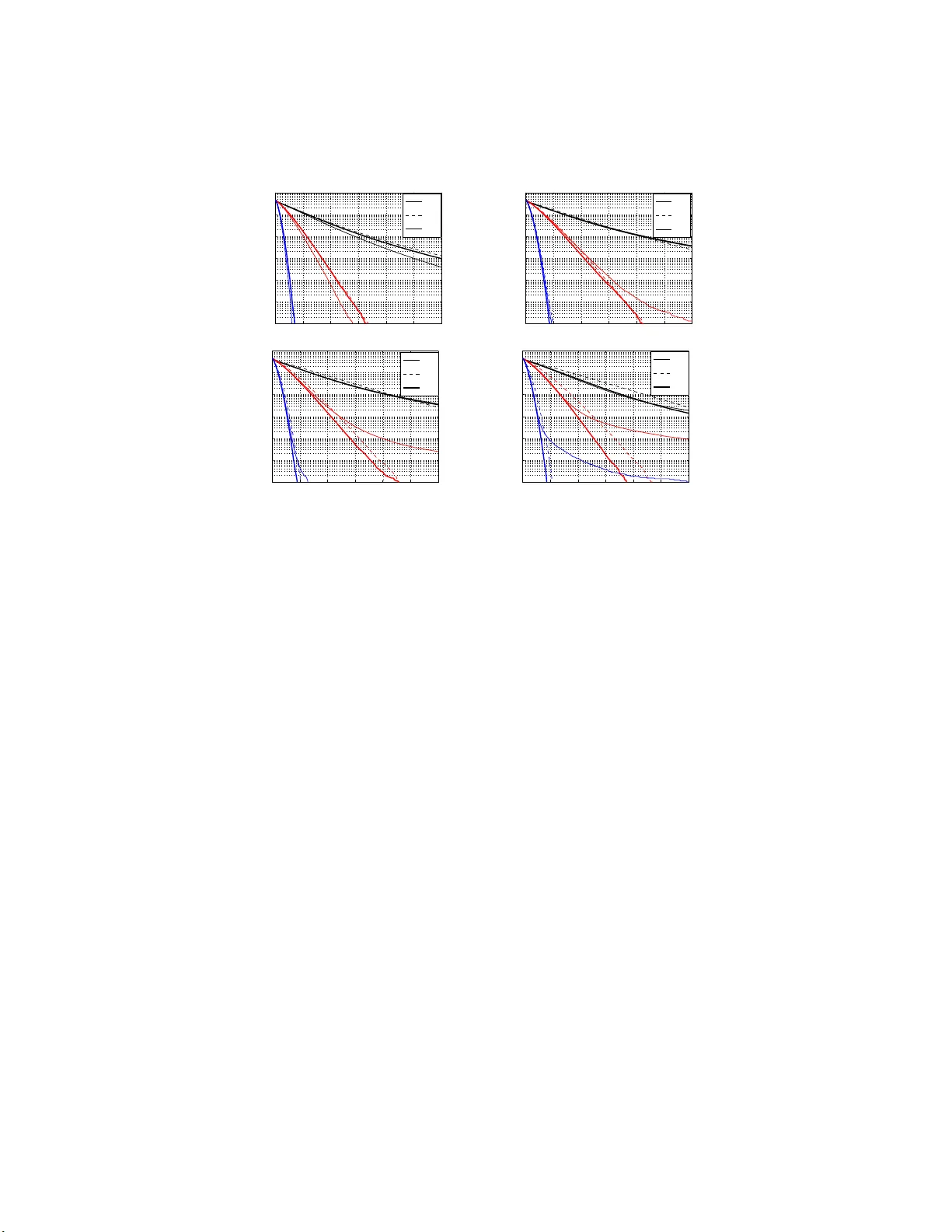
Computationally Efficien t Estimators for Dimension Reductions Using Stable Random Pro jections Ping Li Department of Statistical Science, Cornell Univers ity , Ithaca NY 14853, USA { pingli } @ cornell.edu Abstract. The 1 metho d of stable r andom pr oj e ctions is a tool for effi- cien tly computing the l α distances using lo w memory , w here 0 < α ≤ 2 is a tuning parameter. The meth od b oils do wn to a statistical estimation task and v arious estimators h a ve b een prop osed, b ased on the ge ometric me an , th e harmonic me an , and the fr actional p ower etc. This study prop oses the optimal quantile e stimator, whose main op- eration is sele cting , which is considerably less exp ensive than taking fractional p ow er, the main operation in previous esti mators. Our exp er- iments rep ort t hat the optimal quantile estimator is n early one order of magnitud e more computationally efficien t than previous estimators. F or large-scale learning tasks in whic h storing and compu ting p airwise distances is a serious b ottlenec k, this estimator should b e d esirable. In addition to its computational advan tages, the optimal quantile estima- tor exhibits nice theoretical prop erties. It is more accurate th an p rev ious estimators when α > 1. W e derive its theoretical error b ounds and es- tablish the explicit (i.e., no hidden constants) sample complexity b ound. 1 In tro duction The metho d of stable r andom pr oje ct ions [1,2,3], as a n efficient to o l for comput- ing pairwise distances in massive high-dimensional data, provides a promising mechanism to tackle some of the challenges in moder n machine learning. In this pap er, we provide an eas y-to-implement algor ithm for st able ra ndom pr oje ctions which is b oth statistica lly accurate and computationally efficient . 1.1 Massive Hi g h-dimensi onal Data i n Mo dern M achine Learning W e denote a data matrix by A ∈ R n × D , i.e., n data p oints in D dimens ions. Data sets in mo dern applications exhibit imp orta n t characteristics whic h imp ose tremendous challenges in machine learning [4]: – Modern da ta s e ts with n = 10 5 or even n = 10 6 po int s ar e not uncommon in sup e rvised lear ning, e.g ., in image/text classifica tion, r a nking algorithms for search engines, etc. In the unsup ervised do main (e.g., W eb cluster ing, ads clickthroughs, word/term asso ciations ), n can be even m uch lar ger. – Modern data sets are o ften of ultra high-dimensions ( D ), s ometimes in the order o f millions (or even higher), e.g ., image , text, genome (e.g., SNP ), etc. F or example, in image analysis, D may be 10 3 × 10 3 = 10 6 if using pixels as features, or D = 256 3 ≈ 16 million if using color histogra ms as f eatures . – Modern data se ts ar e s ometimes collected in a dynamic streaming fashion. 1 First draft F eb. 2008 , sligh tly revised in June 2008. The results w ere announced in Jan uary 2008 at SODA’0 8 when the auth or presented the w ork of [2]. 2 – Large-scale data are often hea vy-taile d, e.g., image and text data. Some larg e-scale data ar e dense, such as image a nd genome da ta. Even for data sets which are sparse, suc h as text, the abs o lute nu mber of no n-zeros may be still large. F or example, if o ne querie s “machine learning” (a no t-to o-common term) in Go ogle.com, the to tal n umber of pa gehits is ab out 3 million. In other words, if one builds a term-do c matrix at W eb scale, although the ma trix is sparse, most rows will con tain large num bers (e.g., millions) of non-zero en tries. 1.2 P airwise Dis tances in Mac hine Learning Many lear ning algor ithms re q uire a simila r ity matrix computed from pairwis e distances of the da ta matrix A ∈ R n × D . Examples include clustering, neares t neighbors, mult idimensional sca ling, a nd k ernel SVM (suppor t vector machines). The similarity matrix requires O ( n 2 ) storage space a nd O ( n 2 D ) computing time. This study fo cuses on the l α distance (0 < α ≤ 2). Co ns ider t wo v ectors u 1 , u 2 ∈ R D (e.g., the leading tw o rows in A ), the l α distance betw een u 1 and u 2 is d ( α ) = D X i =1 | u 1 ,i − u 2 ,i | α . (1) Note that, strictly sp eaking, the l α distance should b e defined as d 1 /α ( α ) . Be- cause the power op era tion ( . ) 1 /α is the same for all pairs, it often makes no difference whether we use d 1 /α ( α ) or just d ( α ) ; and hence w e fo cus on d ( α ) . The radial basis kernel (e.g., for SVM) is constructed from d ( α ) [5,6]: K ( u 1 , u 2 ) = exp − γ D X i =1 | u 1 ,i − u 1 ,i | α ! , 0 < α ≤ 2 . (2) When α = 2, this is the Gaussia n ra dial ba sis kernel. Her e α can b e viewed as a tuning parameter . F or example, in their histo gram-bas ed image classifica tio n pro ject using SVM, [5 ] rep orted that α = 0 and α = 0 . 5 a c hieved go o d per for- mance. F or hea vy-taile d data, tuning α has the similar effect as term-weighting the original data, often a critical step in a lot of applications [7,8]. F or p opular k ernel SVM so lvers including the Se quent ial Minimal Optimiza- tion (SMO ) a lgorithm[9], stor ing and co mputing kernels is the ma jor b ottleneck. Three computational challenges were summarized in [4, page 12]: – Computi ng kernels is exp ensive – Computi ng ful l kern el matrix is w asteful Efficient SVM solvers often do not need to ev alua te all pair wise k ernels. – Kernel matrix do es not fit in memory Storing the k ernel matrix at the memory co s t O ( n 2 ) is challenging when n > 10 5 , and is not realistic for n > 10 6 , be c a use O ` 10 12 ´ consumes at least 1000 GBs memory . A p opular strateg y in la r ge-scale learning is to ev a luate distances on the fly [4]. That is, instead of loading the similarit y matr ix in memory at the co st of O ( n 2 ), one can load the or iginal data matrix at the cos t of O ( nD ) and recompute pairwise distances on-demand. This s trategy is apparent ly problematic when D 3 is not to o sma ll. F or high-dimensional data, either lo ading the data matrix in memory is unrea listic or computing distances on-dema nd b ecomes too exp ensive. Those challenges are not unique to kernel SVM; they ar e general issues in distanced-based learning algo rithms. The metho d of stable r andom pr oje ctions provides a pr omising scheme by reducing the dimension D to a s mall k (e.g., k = 50 ), to f acilitate co mpact data storage and efficien t distance computations. 1.3 Stable Random Pro jec tions The basic pro cedur e of s t able r andom pr oje ctions is to mu ltiply A ∈ R n × D by a rando m ma trix R ∈ R D × k ( k ≪ D ), which is generated by sampling each ent ry r ij i.i.d. from a sy mmetr ic stable distr ibution S ( α, 1). The resultant matrix B = A × R ∈ R n × k is m uch smaller than A a nd hence it ma y fit in memory . Suppo se a stable rando m v ariable x ∼ S ( α, d ), where d is the scale pa r ameter. Then its characteristic function (F ourier tra nsform of the densit y function) is E ` exp ` √ − 1 xt ´´ = exp ( − d | t | α ) , which do es not have a closed-for m inv erse except for α = 2 (normal) or α = 1 (Cauch y). Note that when α = 2, d corr esp onds to “ σ 2 ” (not “ σ ”) in a normal. Corresp onding to the le a ding t wo rows in A , u 1 , u 2 ∈ R D , the lea ding t wo rows in B ar e v 1 = R T u 1 , v 2 = R T u 2 . The entries of the difference, x j = v 1 ,j − v 2 ,j = D X i =1 r ij ( u 1 ,i − u 2 ,i ) ∼ S α, d ( α ) = D X i =1 | u 1 ,i − u 2 ,i | α ! , for j = 1 to k , are i.i.d. samples fro m a stable distribution with the scale pa- rameter b eing the l α distance d ( α ) , due to prop erties of F ourier transforms. F or example, when α = 2, a weighted sum of i.i.d. standard nor mals is also normal with the scale pa rameter (i.e., v ariance) b eing the sum of squar es of a ll weights. Once we o bta in the stable samples, one can disc a rd the o riginal matrix A and the remaining task is to estimate the scale parameter d ( α ) for each pair . Some applications of stable r andom pr oje ctions are summarized as follows: – Computi ng al l p air wise di stanc es The cost of computing all pair- wise distances of A ∈ R n × D , O ( n 2 D ) , is significa nt ly reduced to O ( nD k + n 2 k ) . – Estimating l α distanc es online F or n > 10 5 , it is challenging or unrealistic to mater ialize all pair w is e distances in A . Thus, in applicatio ns such as online learning, databases, sear ch engines , and online recommenda - tion systems , it is often mor e efficien t if we store B ∈ R n × k in the memory and estimate any distance on the fly if needed. Estima ting distances o nline is the sta ndard stra tegy in large- scale k ernel learning [4]. With st able r andom pr oje ctions , this simple strategy becomes effectiv e in high-dimensional data . – L e arnin g with dynamic str e aming data In re a lity , the data ma- trix may be up dated overtime. In fa c t, with s treaming data ar riving a t high- rate[1,10], the “data matrix” may b e never stored a nd hence all op era tions (such as clustering a nd class ification) m ust b e conducted on the fly . The 4 metho d of s t able r andom pr oje ct ions provides a scheme to compute and up- date dista nces on the fly in one-pa s s of the da ta; see r elev a nt pap ers (e.g., [1]) for more details on this importa n t and fast-developing sub ject. – Estimating entr opy The entrop y distance P D i =1 | u 1 ,i − u 2 ,i | log | u 1 ,i − u 2 ,i | is a useful statistic. A workshop in NIPS’0 3 ( www.menem.c om/ ~ ilya/pages /NIPS03 ) fo cused on ent ropy estimation. A rece n t practica l algor ithm is simply us- ing the difference b et ween the l α 1 and l α 2 distances[11], where α 1 = 1 . 05, α 2 = 0 . 95 , and the distances were es timated b y stable ra ndom pr oj e ctions . If one tunes the l α distances for many different α (e.g., [5]), then stable r andom pr oje ctions will b e even more desirable as a cost-saving device. 2 The Statistical Estimation Problem Recall that the metho d of s t able r andom pr oje ctions b oils down to a statistical estimation pr oblem. That is, es timating the sca le par ameter d ( α ) from k i.i.d. samples x j ∼ S ( α, d ( α ) ), j = 1 to k . W e consider tha t a go od estimator ˆ d ( α ) should hav e the follo wing desirable prop e rties: – (Asymptotically ) un biased and small v ariance. – Computatio nally efficien t. – Ex po nen tial decrease of error (tail) probabilities. The arithmetic me an estimator 1 k P k j =1 | x j | 2 is go o d for α = 2. When α < 2, the task is less stra ig ht forward b ecause (1) no explicit dens it y of x j exists unless α = 1 or 0+; and (2) E( | x j | t ) < ∞ only when − 1 < t < α . 2.1 Sev eral Previous Estim ators Initially rep orted in arXiv in 2006, [2] propo sed the ge ometric me an estimator ˆ d ( α ) ,gm = Q k j =1 | x j | α/k ˆ 2 π Γ ` α k ´ Γ ` 1 − 1 k ´ sin ` π 2 α k ´˜ k . where Γ ( . ) is the Ga mma function, and the harmonic me an estimator ˆ d ( α ) ,hm = − 2 π Γ ( − α ) sin ` π 2 α ´ P k j =1 | x j | − α k − − π Γ ( − 2 α ) sin ( π α ) ˆ Γ ( − α ) sin ` π 2 α ´˜ 2 − 1 !! . More recent ly , [3] prop osed the fr actional p ower e stimator ˆ d ( α ) ,f p = 1 k P k j =1 | x j | λ ∗ α 2 π Γ (1 − λ ∗ ) Γ ( λ ∗ α ) sin ` π 2 λ ∗ α ´ ! 1 /λ ∗ × 1 − 1 k 1 2 λ ∗ „ 1 λ ∗ − 1 « 2 π Γ (1 − 2 λ ∗ ) Γ (2 λ ∗ α ) sin ( π λ ∗ α ) ˆ 2 π Γ (1 − λ ∗ ) Γ ( λ ∗ α ) sin ` π 2 λ ∗ α ´˜ 2 − 1 !! , where λ ∗ = argmin − 1 2 α λ< 1 2 1 λ 2 2 π Γ (1 − 2 λ ) Γ (2 λα ) sin ( π λα ) ˆ 2 π Γ (1 − λ ) Γ ( λ α ) sin ` π 2 λα ´˜ 2 − 1 ! . 5 0 0.2 0.4 0.6 0.8 1 1.2 1.4 1.6 1.8 2 0.4 0.5 0.6 0.7 0.8 0.9 1 α Efficiency Frational power Geometric mean Harmonic mean Optimal quantile Fig. 1. The Cram´ er-Rao efficiencies (the higher the b etter, max = 100%) of v a rious estimato rs, including the optimal quantile estimator prop osed in this study . All thr ee estimators ar e unbiased or asymptotically (as k → ∞ ) unbiased. Figure 1 compares their asymptotic v ariances in terms of the Cram´ er-Rao effi- ciency , which is the r atio of the smallest p oss ible a symptotic v a riance ov er the asymptotic v a riance of the estimator, as k → ∞ . The ge ometric me an estimator, ˆ d ( α ) ,gm exhibits tail bo unds in exp onential forms, i.e., the error s decrea se exponentially fast: Pr “ | ˆ d ( α ) ,gm − d ( α ) | ≥ ǫd ( α ) ” ≤ 2 ex p „ − k ǫ 2 G gm « . The harmonic me an estimator , ˆ d ( α ) ,hm , works well for small α , and has ex- po nent ial tail b ounds for α = 0 +. The fr actional p ower estimator , ˆ d ( α ) ,f p , has smaller a s ymptotic v a r iance than bo th the ge ometric me an and harmonic me an estimators. Howev er, it do es no t hav e exp onential tail b ounds, due to the r estriction − 1 < λ ∗ α < α in its definition. As s hown in [3], it only has finite moment s slightly higher than the 2 nd or der , when α approaches 2 (b eca us e λ ∗ → 0 . 5 ), meaning that larg e error s ma y ha ve a go o d c hance to o ccur. W e will demons trate this b y simulations. 2.2 The Issue of Computatio nal Effi ciency In the definitions o f ˆ d ( α ) ,gm , ˆ d ( α ) ,hm and ˆ d ( α ) ,f p , all three es tima to rs require ev a luating fractional p ow ers, e.g., | x j | α/k . This o per ation is r elatively expens ive, esp ecially if w e need to conduct this tens of billions of times (e.g., n 2 = 1 0 10 ). F o r exa mple, [5] rep orted that, althoug h the r adial basis kernel (2) with α = 0 . 5 ac hieved go o d p er formance, it was not preferred b ecause ev aluating the square ro ot w as to o exp ensive. 2.3 Our Prop osed Estimator W e pr op ose the op timal quantile estimator, using the q ∗ th smallest | x j | : ˆ d ( α ) ,oq ∝ ( q ∗ -quantile {| x j | , j = 1 , 2 , ..., k } ) α , (3) where q ∗ = q ∗ ( α ) is chosen to minimize the a symptotic v ar iance. 6 This estimator is co mputatio nally attractive b ecause selecting should b e m uch less exp ensive than ev aluating frac tio nal p ow ers. If we ar e interested in d 1 /α ( α ) instead, then we do not even need to ev aluate any fr actional p owers. As mentioned, in many case s using either d ( α ) or d 1 /α ( α ) makes no difference and d ( α ) is o ften preferr ed b ecause it av oids taking ( . ) 1 /α power. The radial ba sis kernel (2) requires d ( α ) . T hus this study fo cuses on d ( α ) . O n the other hand, if we can estimate d 1 /α ( α ) directly , for exa mple, using (3) without the α th pow er, we might as well j ust use d 1 /α ( α ) if per mitted. In case w e do not need to ev aluate an y fractional p ow er, our estimator will b e even more computationally efficient . In addition to the co mputatio nal adv an tages , this estimator also has go o d theoretical prop erties, in terms of bo th the v ariances and tail probabilities: 1. Figur e 1 illustra tes that, compa red with the ge ometric me an estimator, its asymptotic v ariance is a bo ut the same when α < 1, and is considerably smaller when α > 1. Compared with the fr actional p ower estimator, it has smaller asymptotic v ariance when 1 < α ≤ 1 . 8 . In fact, as will b e shown b y simulations, when th e sample size k is not to o large, its mean squar e error s are considera bly smaller than the fr actional p ower e stimator when α > 1. 2. The optimal quantile estimator exhibits ta il b ounds in exp onential forms. This theoretical contribution is practically impo rtant, for selecting the sam- ple size k . In le arning theory , the gener alization bo unds are often lo o se. In our case , how ever, the bounds are tig h t b ecause the distribution is specified. The next section will be devoted to ana lyzing the optimal quantile estimator. 3 The Optimal Quan t ile Estimator Recall the go a l is to estimate d ( α ) from { x j } k j =1 , wher e x j ∼ S ( α, d ( α ) ) , i.i.d. Since the distribution b elong s to the scale family , o ne can estimate the scale para meter from quantiles. Due to sy mmetr y , it is natura l to consider the absolute v alues: ˆ d ( α ) ,q = „ q -Quantile { | x j | , j = 1 , 2 , ..., k } q -Quantile {| S ( α, 1) |} « α , (4) which is b est understo o d by the fact that if x ∼ S ( α, 1) , then d 1 /α x ∼ S ( α, d ) , or more ob viously , if x ∼ N (0 , 1), then ` σ 2 ´ 1 / 2 x ∼ N ` 0 , σ 2 ´ . By prop erties of or der statistics [1 2], any q -quan tile will pro vide an as ymptotically unbiased estimator. Lemma 1 provides the asymptotic v ariance of ˆ d ( α ) ,q . Lemma 1 . Denote f X ` x ; α, d ( α ) ´ and F X ` x ; α, d ( α ) ´ the pr ob ability d ensity func- tion and the cumulative density funct ion of X ∼ S ( α, d ( α ) ) , r esp e ctively . The asymptotic varianc e of ˆ d ( α ) ,q define d in (4) is V ar “ ˆ d ( α ) ,q ” = 1 k ( q − q 2 ) α 2 / 4 f 2 X ( W ; α, 1) W 2 d 2 ( α ) + O „ 1 k 2 « (5) wher e W = F − 1 X (( q + 1) / 2; α, 1) = q -Quantile {| S ( α, 1) |} . Pr o of: Se e App endix A.  . 7 3.1 Optimal Quan tile q ∗ ( α ) W e cho ose q = q ∗ ( α ) so that the asymptotic v ariance (5) is minimized, i.e., q ∗ ( α ) = argmin q g ( q ; α ) , g ( q ; α ) = q − q 2 f 2 X ( W ; α, 1) W 2 . (6) The conv exity of g ( q ; α ) is imp ortant. Graphically , g ( q ; α ) is a con vex function of q , i.e., a unique minimu m exists. An algebr aic pro of, how ev er, is difficult. Nevertheless, w e can obtain a nalytical solutions when α = 1 and α = 0 +. Lemma 2 . When α = 1 or α = 0+ , the function g ( q ; α ) define d in (6) is a c onvex function of q . When α = 1 , the optimal q ∗ (1) = 0 . 5 . When α = 0 + , q ∗ (0+) = 0 . 203 is the solution to − log q ∗ + 2 q ∗ − 2 = 0 . Pr o of: Se e App endix B.  . It is also easy to sho w that when α = 2, q ∗ (2) = 0 . 862 . W e denote the optimal qu antile estimator by ˆ d ( α ) ,oq , which is sa me as ˆ d ( α ) ,q ∗ . F o r general α , w e resor t to numerical solutions, as presented in Figure 2. 0 0.2 0.4 0.6 0.8 1 1.2 1.4 1.6 1.8 2 0 0.1 0.2 0.3 0.4 0.5 0.6 0.7 0.8 0.9 1 α q* (a) q ∗ 0 0.2 0.4 0.6 0.8 1 1.2 1.4 1.6 1.8 2 0.5 1 1.5 2 2.5 3 3.5 4 4.5 α W α (q*) (b) W α ( q ∗ ) Fig. 2. (a) The optimal v alues for q ∗ ( α ), which minimizes asy mpto tic v ari- ance of ˆ d ( α ) ,q , i.e., the solution to (6). (b) The constant W α ( q ∗ ) = { q ∗ -quantile {| S ( α, 1) |}} α . 3.2 Bias Correction Although ˆ d ( α ) ,oq (i.e., ˆ d ( α ) ,q ∗ ) is asymptotically (as k → ∞ ) unbiased, it is seriously biased for small k . Thus, it is pr actically impo rtant to remov e the bias . The unbiased version of the op timal qu antile estimator is ˆ d ( α ) ,oq ,c = ˆ d ( α ) ,oq /B α,k , (7) where B α,k is the exp ectation o f ˆ d ( α ) ,oq at d ( α ) = 1 . F o r α = 1, 0 +, o r 2 , we ca n ev aluate the exp ectations (i.e., integrals) analytica lly or by numerical int egra tions. F or gener al α , as the probability densit y is no t av ailable , the task is difficult and pro ne to n umerical ins tabilit y . O n the other hand, since the Monte-Carlo sim ulation is a p o pular alternative for ev aluating difficult integrals, a practical solution is to sim ulate the exp ectations, as presented in Fig ure 3. Figure 3 illustrates that B α,k > 1, meaning that this correction also reduces v a riance while re moving bias (because V ar( x/c ) = V ar( x ) /c 2 ). F or exa mple, when 8 0 0.2 0.4 0.6 0.8 1 1.2 1.4 1.6 1.8 2 1 1.05 1.1 1.15 1.2 1.25 α B α ,k k = 10 20 k = 15 50 30 100 25 50 75 100 125 150 175 200 1 1.05 1.1 1.15 1.2 1.25 k B α ,k α = 0.1 α = 1.95 Fig. 3. The bias c orrection factor B α,k in (7), obtained from 1 0 8 simulations for every combination of α (spaced at 0.05) and k . B α,k = E “ ˆ d ( α ) ,oq ; d ( α ) = 1 ” . α = 0 . 1 and k = 1 0 , B α,k ≈ 1 . 2 4, which is sig nificant, b ecause 1 . 2 4 2 = 1 . 54 implies a 54% difference in ter ms of v ariance, a nd even mor e considera ble in terms of the mean square error s MSE = v ar iance + bias 2 . B α,k can b e tabulated for small k , and absorb ed into other co efficients, i.e., this do es not increase the computational co st at run time. W e fix B α,k as rep orted in Figure 3. The sim ulations in Section 4 directly used those fixed B α,k v a lues. 3.3 Computational Effi ciency Figure 4 compar es the co mputatio nal co sts of the ge ometric m e an , the fr actional p ower , and the optimal quantile estimators. The harmonic me an estimato r was not included as it costs very similar ly to the fr actional p ower estimator. W e use d the build-in function “pow”in gcc for e v aluating the fra ctional pow- ers. W e implemented a “quick se le ct” algo r ithm, which is similar to quick s ort and requires on av erage linea r time. F or simplicity , o ur implementation us ed recursions and the middle elemen t as pivot. Also , to ensur e f airnes s, for all esti- mators, co efficients w hich are functions of α and/or k were pre-computed. 0 0.2 0.4 0.6 0.8 1 1.2 1.4 1.6 1.8 2 0 1 2 3 4 5 6 7 8 α Ratio of computing time gm / fp gm / oq 0 50 100 200 300 400 500 0 1 2 3 4 5 6 7 8 9 k Ratio of computing time gm / fp gm / oq Fig. 4. Re la tive co mputational cos t ( ˆ d ( α ) ,gm ov er ˆ d ( α ) ,oq ,c and ˆ d ( α ) ,gm ov er ˆ d ( α ) ,f p ), from 1 0 6 simulations at each combination o f α and k . The left panel av erag es ov er all k and the r ight panel a verages over all α . Note that the co st of ˆ d ( α ) ,oq ,c includes ev aluating the α th momen t once. Normalized by the computing time of ˆ d ( α ) ,gm , we observ e that rela tive com- putational efficiency does no t stro ngly depend on α . W e do obse rve that the ra tio 9 of computing time of ˆ d ( α ) ,gm ov er that of ˆ d ( α ) ,oq ,c increases consistently with in- creasing k . This is b ecaus e in the de finitio n o f ˆ d ( α ) ,oq (and hence als o ˆ d ( α ) ,oq ,c ), it is required to ev aluate the fractional pow er o nce, whic h cont ributes to the to ta l computing time more significantly a t smaller k . Figure 4 illustr ates that, (A) the ge ometric me an estimator and the fr ac- tional p ower estimator are similar in terms of computational efficienc y ; (B) the optimal qu ant ile estimator is nearly one order of ma gnitude more computation- ally efficient than the ge ometric me an and fr actional p ower estimators. Because we implemented a “na ´ ıve” version o f “quick s elect” using recursions and s imple pivoting, the actual improv emen t may be more sig nificant. Also, if applications require only d 1 /α ( α ) , then no fractional power o p er ations are needed for ˆ d ( α ) ,oq ,c and the improv ement will be even more conside r able. 3.4 Error (T ail ) Bounds Erro r (tail) b ounds are esse n tial for determining k . The v ariance alone is not sufficient for that purp ose. If a n estimato r of d , s ay ˆ d , is normally distributed, ˆ d ∼ N ` d, 1 k V ´ , the v ariance suffices for c ho osing k because its er ror (tail) probability Pr “ | ˆ d − d | ≥ ǫd ” ≤ 2 exp “ − k ǫ 2 2 V ” is deter mined by V . In genera l, a reasona ble estimator will be asymptotically no rmal, for small eno ugh ǫ a nd larg e enough k . F o r a finite k and a fixed ǫ , how ever, the nor mal appr oximation may be (very) po o r. This is especia lly true for the fr actional p ower estimator, ˆ d ( α ) ,f p . Thu s, for a g o o d motiv a tion, Lemma 3 provides the error (tail) proba bilit y bo unds of ˆ d ( α ) ,q for any q , not just the optimal qua n tile q ∗ . Lemma 3 . Denote X ∼ S ( α, d ( α ) ) and its pr ob ability density funct ion by f X ( x ; α, d ( α ) ) and cumulative function by F X ( x ; α, d ( α ) ) . Given x j ∼ S ( α, d ( α ) ) , i.i.d., j = 1 to k . U sing ˆ d ( α ) ,q in (4), then Pr “ ˆ d ( α ) ,q ≥ (1 + ǫ ) d ( α ) ” ≤ exp „ − k ǫ 2 G R,q « , ǫ > 0 , (8) Pr “ ˆ d ( α ) ,q ≤ (1 − ǫ ) d ( α ) ” ≤ exp „ − k ǫ 2 G L,q « , 0 < ǫ < 1 , (9) ǫ 2 G R,q = − (1 − q ) log (2 − 2 F R ) − q log(2 F R − 1) + (1 − q ) log (1 − q ) + q log q , (10) ǫ 2 G L,q = − (1 − q ) log (2 − 2 F L ) − q log(2 F L − 1) + ( 1 − q ) log (1 − q ) + q log q , (11) W = F − 1 X (( q + 1) / 2; α, 1) = q -quantile {| S ( α, 1) |} , F R = F X “ (1 + ǫ ) 1 /α W ; α, 1 ” , F L = F X “ (1 − ǫ ) 1 /α W ; α, 1 ” . As ǫ → 0+ lim ǫ → 0+ G R,q = lim ǫ → 0+ G L,q = q (1 − q ) α 2 / 2 f 2 X ( W ; α, 1) W 2 . (12) Pr o of: Se e A pp endix C.  10 The limit in (12) as ǫ → 0 is precisely twice the asymptotic v ariance factor of ˆ d ( α ) ,q in (5), consistent with the nor mality a pproximation men tioned prev iously . This explains why w e express the co nstants a s ǫ 2 /G . (12) also indica tes that the tail bo unds achiev e the “optimal rate” for this estimator, in the language of large deviation theory . By the Bonferroni bound, it is ea sy to determine the sample s ize k Pr “ | ˆ d ( α ) ,q − d ( α ) | ≥ ǫd ( α ) ” ≤ 2 ex p „ − k ǫ 2 G « ≤ δ / ( n 2 / 2) = ⇒ k ≥ G ǫ 2 (2 log n − log δ ) . Lemma 4 . Using ˆ d ( α ) ,q with k ≥ G ǫ 2 (2 log n − log δ ) , any p airwise l α distanc e among n p oints c an b e appr oximate d within a 1 ± ǫ factor with pr ob abili ty ≥ 1 − δ . It suffic es to let G = max { G R,q , G L,q } , wher e G R,q , G L,q ar e define d in L emma 3. The Bonfer r oni bound can b e unnecessarily conserv ative. It is often r eason- able to replace δ / ( n 2 / 2) by δ /T , meaning that ex cept for a 1 /T fra ction of pairs, any dista nce can be approximated within a 1 ± ǫ factor with pro bability 1 − δ . Figure 5 plots the error b ound constants for ǫ < 1, for b o th the reco m- mended optimal quantile estimator ˆ d ( α ) ,oq and the baseline sample me dia n esti- mator ˆ d ( α ) ,q = 0 . 5 . Although we choose ˆ d ( α ) ,oq based on the a symptotic v a riance, it turns out ˆ d ( α ) ,oq also exhibits (muc h) b etter tail b ehaviors (i.e., s maller con- stants) than ˆ d ( α ) ,q = 0 . 5 , at least in the range of ǫ < 1 . 0 0.1 0.2 0.3 0.4 0.5 0.6 0.7 0.8 0.9 1 3 5 7 9 11 13 15 17 19 ε G R, q* α = 0 α = 2 G R, q = q* 0 0.1 0.2 0.3 0.4 0.5 0.6 0.7 0.8 0.9 1 0 1 2 3 4 5 6 7 8 9 10 11 ε G L, q* G L, q = q* α = 2 α = 0 0 0.1 0.2 0.3 0.4 0.5 0.6 0.7 0.8 0.9 1 4 6 8 10 12 14 16 18 ε G R, 0.5 α = 0 G R, q = 0.5 α = 2 0 0.1 0.2 0.3 0.4 0.5 0.6 0.7 0.8 0.9 1 0 1 2 3 4 5 6 7 8 9 10 11 ε G L, 0.5 G L, q = 0.5 α = 2 α = 0 Fig. 5. T ail b ound consta nts for quantile es timators; the low er the b etter. Up- per panels: optimal qua n tile estimators ˆ d ( α ) ,q ∗ . Low er panels: median estimato rs ˆ d ( α ) ,q =0 . 5 . Consider k = G ǫ 2 (log 2 T − log δ ) (reca ll w e suggest replacing n 2 / 2 b y T ), w ith δ = 0 . 05, ǫ = 0 . 5, and T = 10. Bec a use G R,q ∗ ≈ 5 ∼ 9 aro und ǫ = 0 . 5, we o btain 11 k ≈ 1 20 ∼ 215, which is still a re latively lar ge num b er (althoug h the origina l dimension D might be 10 6 ). If we choose ǫ = 1 , then approximately k ≈ 40 ∼ 65. It is p oss ible k = 120 ∼ 215 might b e still co nserv ativ e, for three reasons : (A) the tail bo unds, although “shar p,” a re still upp er b ounds; (B) using G = max { G R,q ∗ , G L,q ∗ } is conserv ative beca use G L,q ∗ is usua lly muc h smaller than G R,q ∗ ; (C) this t yp e of tail b ounds is based on relative erro r, which ma y be stringent fo r sma ll ( ≈ 0) distances. In fact, some ear lier studies on normal r andom pr oje ctions (i.e., α = 2) [13,14] empirically demonstrated that k ≥ 50 appe a red sufficient . 4 Sim ulations W e resort to sim ulations for comparing the finite sample v ariances o f v a rious estimators and assessing the more precise error (tail) probabilities. One adv an tage of stable r andom pr oje ctions is that we know the (manually generated) dis tr ibutions and the only source of error s is fro m the random n umber generations . Thus, we ca n simply rely on sim ulations to ev aluate th e estimators without using real da ta. In fact, after pr o jections, the pr o jected data follow exactly the stable distribution, regar dless o f the original real data distribution. Without loss o f gener ality , we simulate sa mples fro m S ( α, 1) and e s timate the scale parameter (i.e., 1) from the samples. Rep eating the pr o cedure 10 7 times, we can reliably ev aluate the mean square errors (MSE) and tail probabilities. 4.1 Mean Square Errors (M SE) As illustra ted in Figur e 6, in terms of the MSE , the optimal quantile estimator ˆ d ( α ) ,oq ,c outp e rforms b oth the ge ometric me an and fr actio nal p ower estimators when α > 1 a nd k ≥ 20. The fr actional p ower estima to r do es no t a ppea r to b e very suita ble for α > 1, esp ecially for α clo se to 2 , even when the sample size k is not to o small (e.g., k = 50 ). F or α < 1, how ever, the fr actional p ower estimator has go o d perfo r mance in terms of MSE, ev en for small k . 4.2 Error(T ail) Probabil ities Figure 7 pr esents the simulated r ight tail pro babilities, Pr “ ˆ d ( α ) ≥ (1 + ǫ ) d ( α ) ” , illustrating that when α > 1, the fr actional p ower estimator ca n exhibit very bad tail b ehaviors. F or α < 1, the fr actiona l p ower estimator demonstr ates go o d per formance at least for the probability r a nge in the sim ulations. Thu s, Fig ure 7 de mo nstrates that the optimal quantile estimator consistently outp e rforms the fr actional p ower and the ge ometric me an estimator s when α > 1 . 5 The Related W ork There have b een many s tudies of normal r andom pr oje ctions in machine learning, for dimension r eduction in the l 2 norm, e.g., [14], highlighted by the Jo hnson- Lindenstrauss (JL) Lemma [15], which says k = O  log n/ǫ 2  suffices when using normal (or normal-like, e.g., [1 6]) pro jection metho ds. The metho d of stable r andom pr oje ctions is a pplicable for computing the l α distances (0 < α ≤ 2), no t just for l 2 . [1, Lemma 1 , Lemma 2, Theor e m 3] 12 0 0.2 0.4 0.6 0.8 1 1.2 1.4 1.6 1.8 2 1 1.5 2 2.5 3 3.5 4 4.5 5 α MSE × k k = 10 fp gm oq oq asymp. 0 0.2 0.4 0.6 0.8 1 1.2 1.4 1.6 1.8 2 1 1.5 2 2.5 3 3.5 4 4.5 5 α MSE × k k = 20 fp gm oq oq asymp. 0 0.2 0.4 0.6 0.8 1 1.2 1.4 1.6 1.8 2 1 1.5 2 2.5 3 3.5 4 4.5 5 α MSE × k k = 50 fp gm oq oq asymp. 0 0.2 0.4 0.6 0.8 1 1.2 1.4 1.6 1.8 2 1 1.5 2 2.5 3 3.5 4 4.5 5 α MSE × k k = 100 fp gm oq oq asymp. Fig. 6. E mpirical mean sq uare error s (MSE, the lower the better ), from 10 7 simulations at every combination o f α and k . The v alues are m ultiplied b y k so that four plots can b e at ab out the same sca le. The MSE for the ge ometric me an (gm) estimator is computed exactly since clo sed-form express io n exists. The low er dashed cur ves are the as ymptotic v ariances o f the optimal quantile (o q) estimator. suggested the me dian (i.e., q = 0 . 5 quantile) estima tor for α = 1 and arg ued that the s ample complexity b o und should b e O  1 /ǫ 2  ( n = 1 in their study). Their bo und was not provided in an explicit form and r e q uired an “ ǫ is small enough” argument. F or α 6 = 1, [1, Lemma 4 ] o nly pro vided a co nceptual a lgorithm, which “is not uniform.” In this study , w e pro ve the b ounds for any q -qua n tile a nd an y 0 < α ≤ 2 (not just α = 1), in explicit exp onential forms, with no unknown constants and no restr iction that “ ǫ is small enough.” The quantile estimator for stable distributions was prop osed in statistics quite so me time ago, e.g., [1 7,18]. [1 7] mainly fo cused on 1 ≤ α ≤ 2 a nd rec- ommended using q = 0 . 4 4 quantiles (mainly for the sake of smaller bias ). [18] fo cused on 0 . 6 ≤ α ≤ 2 and r ecommended q = 0 . 5 quantiles. This study considers all 0 < α ≤ 2 and recommends q based on the minim um asymptotic v ar ia nce. Beca use the bias can be easily remov ed (at least in the practical sense), it app ears not necessary to us e other quantiles only for the sake of smaller bias. T ail bounds, which are useful for choosing q a nd k based on confidence in terv als, w ere not av ailable in [17,18]. Finally , o ne might ask if there migh t b e be tter es timators. F or α = 1, [19] pro - po sed using a linear combination of qua n tiles (with c a refully c hosen co efficients) to obtain an a symptotically optimal estimator for the Ca uch y scale parameter . While it is p ossible to extend their result to general 0 < α < 2 (requiring so me non-trivial work), whether or not it will b e practica lly better than the optimal 13 0 0.5 1 1.5 2 2.5 3 10 −6 10 −5 10 −4 10 −3 10 −2 10 −1 10 0 ε Probability k = 10 k = 50 k = 500 α = 0.5 fp gm oq 0 0.5 1 1.5 2 2.5 3 10 −6 10 −5 10 −4 10 −3 10 −2 10 −1 10 0 ε Probability k = 10 k = 50 k = 500 α = 1.5 fp gm oq 0 0.5 1 1.5 2 2.5 3 10 −6 10 −5 10 −4 10 −3 10 −2 10 −1 10 0 ε Probability k = 10 k = 50 k = 500 α = 1.75 fp gm oq 0 0.5 1 1.5 2 2.5 3 10 −6 10 −5 10 −4 10 −3 10 −2 10 −1 10 0 ε Probability k = 10 k = 50 k = 500 α = 1.95 fp gm oq Fig. 7. The rig h t tail pr obabilities (the low er the be tter), from 10 7 simulations at each combination of α and k . quantile estimator is unclear b ecaus e the extre me quantiles severely affect the tail probabilities a nd finite-sample v ariances and hence some kind of truncatio n (i.e., discar ding some samples at extreme quantiles) is necessary . Also, exp onen- tial tail b ounds of the linea r com bination of quan tiles m ay not exist or may not be f easible to deriv e. In a ddition, the optimal quantile estimator is computation- ally more efficient . 6 Conclusion Many machine learning alg orithms op era te on the tr aining data only through pairwise distances. Co mputing, s toring, upda ting and retriev ing the “ matrix” of pairwise distances is challenging in a pplications inv olving massive, high-dimensional, and p os sibly s tr eaming, data. F or example, the pairwise distance matrix can no t fit in memory when the n umber of observ ations exceeds 10 6 (or even 10 5 ). The metho d of stable r andom pr oje ctions provides an efficient mec hanism for computing pairwise distances using low memory , by tra nsforming the original high-dimensional data into sketches , i.e., a small num ber of samples from α - stable distributions, which a re m uch ea sier to store and retrieve. This metho d provides a uniform s chem e for co mputing the l α pairwise dis- tances for all 0 < α ≤ 2. Cho osing an a ppropriate α is often critical to the per formance o f learning alg o rithms. In pr inciple, we can tune algorithms fo r many l α distances; and stable ra ndom pr oj e ctions can provide an efficien t too l. T o recover the or ig inal distances , we face a n estimatio n task. Compar ed with previous es timators based on the ge ometric me an , t he harmonic me an , or the fr actio nal p ower , the pro p o s ed optimal quantile estimator ex hibits t wo adv an- tages. Firstly , the optimal quantile estimator is nearly one order o f magnitude 14 more efficient than o ther estimators (e.g ., reducing the training time fro m one week to o ne da y). Sec o ndly , the optimal quantile estimator is considerably more accurate when α > 1 , in terms of b oth the v ar iances and erro r (tail) proba- bilities. Note that α ≥ 1 corre spo nds to a conv ex norm (sa tisfying the triangle inequality), which might b e another motiv ation for using l α distances with α ≥ 1. One theoretica l contribution is the explicit tail b ounds for general quantile estimators and cons equently the sa mple complexity b ound k = O  log n/ǫ 2  . Those b ounds ma y guide pra ctitioners in choo sing k , the n um be r of pro jections. The (practically useful) bo unds are expressed in terms of the probability func- tions and henc e they mig h t b e not as c onv enien t for further theoretical analysis. Also, we should mention that the b ounds do no t r ecov er the optimal b ound of the arithmetic me an estimato r when α = 2 , b ecause the arithmetic me an es- timator is sta tistically optimal a t α = 2 but the optimal quantile es tima to r is not. While w e b elieve that applying stable r andom pr oje ctions in machine lea r ning has b eco me straig ht forward, ther e ar e interesting theoretical issues for future resear ch. F or example, how theoretical properties o f learning algorithms may be affected if the approximated (instea d o f exact) l α distances are used? A Pro of of Lemma 1 Denote f X  x ; α, d ( α )  and F X  x ; α, d ( α )  the probability density function and the cum ulative density function of X ∼ S ( α, d ( α ) ), resp ectively . Similarly we use f Z  z ; α, d ( α )  and F Z  z ; α, d ( α )  for Z = | X | . Due to symmetry , the following relations hold f Z ` z ; α, d ( α ) ´ = 2 f X ` z ; α, d ( α ) ´ = 2 /d 1 /α ( α ) f X “ z /d 1 /α ( α ) ; α, 1 ” , F Z ` z ; α, d ( α ) ´ = 2 F X ` z ; α, d ( α ) ´ − 1 = 2 F X “ z /d 1 /α ( α ) ; α, 1 ” − 1 , F − 1 Z ` q ; α, d ( α ) ´ = F − 1 X ` ( q + 1) / 2; α, d ( α ) ´ = d 1 /α ( α ) F − 1 X (( q + 1) / 2; α, 1) . Let W = q - Quantile {| S ( α, 1) |} = F − 1 X (( q + 1) / 2; α, 1) and W d = F − 1 Z  q ; α, d ( α )  = d 1 /α ( α ) W . Then, following known sta tistical re sults, e.g., [1 2, Theo rem 9.2], the asymptotic v a riance of ˆ d 1 /α α,q should b e V ar “ ˆ d 1 /α α,q ” = 1 k q − q 2 f 2 Z ` W d ; α, d ( α ) ´ W 2 + O „ 1 k 2 « = 1 k q − q 2 d − 2 /α ( α ) f 2 Z ( W ; α, 1) W 2 + O „ 1 k 2 « = 1 k q − q 2 4 d − 2 /α ( α ) f 2 X ( W ; α, 1) W 2 + O „ 1 k 2 « . By “delta method,” i.e ., V ar ( h ( x )) ≈ V ar ( x ) ( h ′ ( x )) 2 , V ar “ ˆ d α,q ” = V ar “ ˆ d α,q ” “ αd ( α − 1) /α ( α ) ” 2 + O „ 1 k 2 « = 1 k ( q − q 2 ) α 2 / 4 f 2 X ( W ; α, 1) W 2 d 2 ( α ) + O „ 1 k 2 « . 15 B Pro of of Lemma 2 First, consider α = 1. In this case, f X ( x ; 1 , 1) = 1 π 1 x 2 + 1 , W = F − 1 X (( q + 1) / 2; 1 , 1) = tan “ π 2 q ” , g ( q ; 1) = q − q 2 „ 2 π 1 tan 2 ( π 2 q ) +1 « 2 tan 2 ` π 2 q ´ = q − q 2 sin 2 ( π q ) π 2 . It suffices to study L ( q ) = log g ( q ; 1). L ′ ( q ) = 1 q − 1 1 − q − 2 π cos( π q ) sin( π q ) , L ′′ ( q ) = − 1 q 2 − 1 (1 − q ) 2 + 2 π 2 sin 2 ( π q ) . Because sin( x ) ≤ x fo r x ≥ 0, it is easy to s ee that π sin( πq ) − 1 q ≥ 0, and π sin( π q ) − 1 1 − q = π sin( π (1 − q )) − 1 1 − q ≥ 0 . Thus, L ′′ ≥ 0, i.e., L ( q ) is conv ex and so is g ( q ; 1 ) = e L ( q ) . Since L ′ (1 / 2) = 0, we k now q ∗ (1) = 0 . 5 . Next we consider α = 0+, us ing a fact [2] that as α → 0+, | S ( α, 1) | α con- verges to 1 / E 1 , where E 1 stands for an exponential distribution with mean 1. Denote h = d (0+) and z j ∼ h /E 1 . The sample quantile estimato r beco mes ˆ d (0+) ,q = q -Quantile { | z j | , j = 1 , 2 , ..., k } q -Quantile { 1 /E 1 } . In this case, f Z ( z ; h ) = e − h/z h z 2 , F − 1 Z ( q ; h ) = − h log q , V ar “ ˆ d (0+) ,q ” = 1 k 1 − q q log 2 q h 2 + O „ 1 k 2 « . It is str a ightforw ard to show that 1 − q q l og 2 q is a conv ex function of q and the minim um is attained by solving − log q ∗ + 2 q ∗ − 2 = 0 , i.e., q ∗ = 0 . 203. C Pro of of Lemma 3 Given k i.i.d. s amples, x j ∼ S ( α, d ( α ) ), j = 1 to k . Let z j = | x j | , j = 1 to k . Denote by F Z ( t ; α, d ( α ) ) the cum ulative density o f z j , and by F Z,k ( t ; α, d ( α ) ) the empirical cumulativ e densit y of z j , j = 1 to k . It is the basic fact[12] ab out order statistics that k F Z,k ( t ; α, d ( α ) ) follows a binomial, i.e., k F Z,k ( t ; α, d ( α ) ) ∼ B in ( k, F Z ( t ; α, d ( α ) )). F o r simplicit y , we replace F Z ( t ; α, d ( α ) ) by F ( t, d ), F Z,k ( t ; α, d ( α ) ) by F k ( t, d ), and d ( α ) by d , in this pro o f. Using the origina l bino mial Chernoff bo unds [20], we obtain, for ǫ ′ > 0 , Pr ` kF k ( t ; d ) ≥ (1 + ǫ ′ ) kF ( t ; d ) ´ ≤ „ k − kF ( t ; d ) k − (1 + ǫ ′ ) kF ( t ; d ) « k − k (1+ ǫ ′ ) F ( t ; d ) „ kF ( t ; d ) (1 + ǫ ′ ) kF ( t ; d ) « (1+ ǫ ′ ) kF ( t ; d ) = " „ 1 − F ( t ; d ) 1 − (1 + ǫ ′ ) F ( t ; d ) « 1 − (1+ ǫ ′ ) F ( t ; d ) „ 1 1 + ǫ ′ « (1+ ǫ ′ ) F ( t ; d ) # k , 16 and for 0 < ǫ ′ < 1 , Pr ` kF k ( t ; d ) ≤ (1 − ǫ ′ ) kF ( t ; d ) ´ ≤ " „ 1 − F ( t ; d ) 1 − (1 − ǫ ′ ) F ( t ; d ) « 1 − (1 − ǫ ′ ) F ( t ; d ) „ 1 1 − ǫ ′ « (1 − ǫ ′ ) F ( t ; d ) # k . Consider the gener al qua n tile es timator ˆ d ( α ) ,q defined in (4). F o r ǫ > 0, (again, denote W = q -q uantile {| S ( α, 1) |} ), Pr “ ˆ d ( α ) ,q ≥ (1 + ǫ ) d ” = Pr ( q -quantile {| x j |} ) ≥ ((1 + ǫ ) d ) 1 /α W ) = Pr “ kF k “ (1 + ǫ ) 1 /α W ; 1 ” ≤ q k ” = Pr ` kF k ( t ; 1) ≤ (1 − ǫ ′ ) kF ( t ; 1) ´ , where t = (1 + ǫ ) 1 /α W and q = (1 − ǫ ′ ) F ( t ; 1 ). Th us Pr “ ˆ d ( α ) ,q ≥ (1 + ǫ ) d ” ≤ 2 6 4 0 @ 1 − F “ ((1 + ǫ )) 1 /α W ; 1 ” 1 − q 1 A 1 − q 0 @ F “ ((1 + ǫ )) 1 /α W ; 1 ” q 1 A q 3 7 5 k = exp − k ǫ 2 G R,q ! . where ǫ 2 G R,q = − (1 − q ) log “ 1 − F “ (1 + ǫ ) 1 /α W ; 1 ”” − q log “ F “ (1 + ǫ ) 1 /α W ; 1 ”” + (1 − q ) log (1 − q ) + q log ( q ) . F o r 0 < ǫ < 1, Pr “ ˆ d ( α ) ,q ≤ (1 − ǫ ) d ” = Pr “ kF k “ (1 − ǫ ) 1 /α W ; 1 ” ≥ q k ” = Pr ` kF k ( t ; 1) ≥ (1 + ǫ ′ ) k F ( t ; 1) ´ , where t = (1 − ǫ ) 1 /α W a nd q = (1 + ǫ ′ ) F ( t ; 1 ). Th us, Pr “ ˆ d ( α ) ,q ≤ (1 − ǫ ) d ” ≤ 2 6 4 0 @ 1 − F “ (1 − ǫ ) 1 /α W ; 1 ” 1 − q 1 A 1 − q 0 @ F “ (1 − ǫ ) 1 /α W ; 1 ” q 1 A q 3 7 5 k = exp − k ǫ 2 G L,q ! , where ǫ 2 G L,q = − (1 − q ) log “ 1 − F “ (1 − ǫ ) 1 /α W ; 1 ”” − q log “ F “ (1 − ǫ ) 1 /α W ; 1 ”” + (1 − q ) log (1 − q ) + q log ( q ) . 17 Denote f ( t ; d ) = F ′ ( t ; d ). Using L’Hospital’s rule lim ǫ → 0+ 1 G R,q = lim ǫ → 0+ − (1 − q ) log “ 1 − F “ (1 + ǫ ) 1 /α W ; 1 ”” ǫ 2 + − q log “ F “ (1 + ǫ ) 1 /α W ; 1 ”” + (1 − q ) log(1 − q ) + q log( q ) ǫ 2 = l im ǫ → 0+ f “ (1 + ǫ ) 1 /α W ; 1 ” W α (1 + ǫ ) 1 /α − 1 F “ (1 + ǫ ) 1 /α W ; 1 ” “ 1 − F “ (1 + ǫ ) 1 /α W ; 1 ”” × F “ (1 + ǫ ) 1 /α W ; 1 ” − q 2 ǫ = l im ǫ → 0+ “ f “ (1 + ǫ ) 1 /α W ; 1 ” W α (1 + ǫ ) 1 /α − 1 ” 2 2 F “ (1 + ǫ ) 1 /α W ; 1 ” “ 1 − F “ (1 + ǫ ) 1 /α W ; 1 ”” = f 2 ( W ; 1) W 2 2 q (1 − q ) α 2 , ( q = F ( W , 1)) . Similarly lim ǫ → 0+ G L,q = 2 q (1 − q ) α 2 f 2 ( W ; 1) W 2 . T o complete the pro of, apply th e relations on Z = | X | in the proof of Lemma 1. References 1. Indyk, P .: S table di stri butions, p se udorandom generators, embe ddings, and data stream com- putation. Jou r nal of ACM 53 (3) (2006) 307–323 2. Li, P .: Estim ators and tail b ounds f or dimension red uction in l α (0 < α ≤ 2) using stable random pro jections. In: SODA. (2008) 10 – 19 3. Li, P ., Hastie, T.J.: A unified near-optim al e stimator for d imension red uction in l α (0 < α ≤ 2) using stable rand om pro jections. In: NIPS , V ancou ver, BC, Canada (2008) 4. Bottou, L., Chap elle, O., DeCoste, D., W eston, J., eds.: Large-Scale Kernel Machines. The MIT Press, Cambridge, MA (2007) 5. Chape lle, O., Haffner, P ., V apnik, V.N.: Su pp ort vector m achines for histogram-based image classification. IEEE T ran s. Neural Netw orks 1 0 (5) (1999) 1055–1064 6. Sch¨ olkopf, B., Smola, A.J.: Learning with K e rnels. The MIT Pr ess, Cambridge, MA (2002) 7. Leop old, E., Kinderm ann, J.: T ext categorization with supp ort vector m achines. how to repre- sent texts in input space? M achine Learn ing 46 (1-3) (2002) 423–444 8. Rennie, J.D., Sh ih, L., T eev an, J., Karger, D.R.: T ackling the p o or assumptions of naive Bay es text classifiers. In: ICML, W ashin gton, DC (2003) 616–623 9. Platt, J.C.: Using analy t ic q p and sparsene ss to sp ee d training of supp ort vector machines. In: NIPS, V ancouver, BC, Canada (1998) 557–563 10. Bab c o ck, B., Babu, S., Datar, M., Motw ani, R., Wi dom, J.: Mo de ls and issues in data stream systems. In : PODS, Madison , WI (2002) 1–16 11. Zh ao, H., Lall, A., Ogih ara, M., Spatscheck, O., W ang, J., Xu , J.: A d ata streaming algorithm for estimati ng entropies of o d flows. In: IM C, San Diego, CA (2007) 12. David, H.A.: Order Stati sti c s. Second ed n. John W iley & S ons, Inc., Ne w Y ork, NY (1981) 13. Bin gham, E., M annila, H.: Random pro jection in dime nsionality reduction: Applicati on s to image and te xt data. In: KDD, San F ran cisco, CA (2001) 245–250 14. F radkin, D., Mad igan, D.: Ex p eriments with rand om pro jections for machine learning. In: KDD, W ashington, DC (2003) 517–522 15. J ohnson, W. B., Li ndenstrauss, J.: Exte nsions of Lipschitz mapping in to Hilbe r t s pace . Con- temp orary Mathematic s 26 (1984) 189–206 16. Achlioptas, D.: Database-friendl y random pro jections: Johnson-Lind enstrauss with binary coins. Journal of Compute r and System S cienc es 66 (4) (2003) 671–687 17. F ama, E.F., Roll, R.: Parameter e stimates f or symmetric stable distributions. Journal of the American Statistical Asso ciation 66 (334) (1971) 331–338 18. M cCullo ch, J.H.: Simple con sistent estimators of stable distribution param eters. Communica- tions on S tatistics-Simulation 1 5 (4) (1986) 1109–1136 19. Che rnoff, H., Gastwirth, J.L., Joh ns, M.V.: Asymptotic distributi on of line ar combinations of functions of order statistics with applications to estimati on. The Annals of Mathem atical Statistics 38 (1) ( 1967) 52–72 20. Che rnoff, H.: A measure of asymptotic efficienc y for tests of a hypothe sis based on th e sum of observ ations. The Annals of Mathematic al St ati stics 23 (4) (1952) 493–507 Computationally Efficien t Estimators for Dimension Reductions Using Stable Random Pro jections Ping Li Department of Statistical Science, Cornell Univers ity , Ithaca NY 14853, USA { pingli } @ cornell.edu Abstract. The 1 metho d of stable r andom pr oj e ctions is a tool for effi- cien tly computing the l α distances using lo w memory , where 0 < α ≤ 2 is a tuning parameter. The meth od b oils do wn to a statistical estimation task and v arious estimators h a ve b een prop osed, b ased on the ge ometric me an , th e harmonic me an , and the fr actional p ower etc. This study prop oses the optimal quant i le estimator, whose main op- eration is sele c ting , whic h is considerably less exp ensive than t aking fractional p ow er, the main operation in previous esti mators. Our exp er- iments rep ort t hat the optimal quantile estimator is n early one order of magnitud e more computationally efficien t than previous estimators. F or large-scale learning tasks in whic h storing and compu ting p airwise distances is a serious b ottlenec k, this estimator should b e d esirable. In addition to its computational advan tages, the optimal quantile estima- tor exhibits nice theoretical prop erties. It is more accurate th an p rev ious estimators when α > 1. W e derive its theoretical error b ounds and es- tablish the explicit (i.e., no hidden constants) sample complexity b ound. 1 In tro duction The metho d of stable r andom pr oje ct ions [1,2,3], as a n efficient to o l for comput- ing pairwise distances in massive high-dimensional data, provides a promising mechanism to tackle some of the challenges in moder n machine learning. In this pap er, we provide an eas y-to-implement algor ithm for st able ra ndom pr oje ctions which is b oth statistica lly accurate and computationally efficient . 1.1 Massive Hi g h-dimensi onal Data i n Mo dern M achine Learning W e denote a data matrix by A ∈ R n × D , i.e., n data p oints in D dimens ions. Data sets in mo dern applications exhibit imp orta n t characteristics whic h imp ose tremendous challenges in machine learning [4]: – Mo der n da ta s e ts with n = 10 5 or even n = 10 6 po int s ar e not uncommon in sup e rvised lear ning, e.g ., in image/text classifica tion, r a nking algorithms for search engines, etc. In the unsup ervised do main (e.g., W eb cluster ing, ads clickthroughs, word/term asso ciations ), n can be even m uch lar ger. – Mo der n data sets are o ften of ultra high-dimensions ( D ), s ometimes in the order o f millions (or even higher), e.g ., image , text, genome (e.g., SNP ), etc. F o r example, in image analysis, D may b e 10 3 × 10 3 = 10 6 if using pixels as features, or D = 256 3 ≈ 16 million if using color histogra ms as f eatures . – Mo der n data se ts ar e s ometimes collected in a dynamic streaming fashion. 1 First draft F eb. 2008 , sligh tly revised in June 2008. The results w ere announced in Jan uary 2008 at SODA’0 8 when the auth or presented the w ork of [2]. 2 – Lar ge-sca le data are often hea vy-taile d, e.g., image and text data. Some larg e-scale data ar e dense, such as image a nd genome da ta. Even for data sets which are sparse, suc h as text, the abs o lute nu mber of no n-zeros may be still large. F or example, if o ne querie s “machine learning” (a no t-to o-common term) in Go ogle.com, the to tal n umber of pa gehits is ab out 3 million. In other words, if one builds a term-do c matrix at W eb sca le, although the ma tr ix is sparse, most rows will con tain large num bers (e.g., millions) of non-zero en tries. 1.2 P airwise Dis tances in Mac hine Learning Many lear ning algor ithms re q uire a simila r ity matrix computed from pairwis e distances of the da ta matrix A ∈ R n × D . Examples include clustering, neares t neighbors, mult idimensional sca ling, a nd k ernel SVM (suppor t vector machines). The similarity matrix requires O ( n 2 ) storage space a nd O ( n 2 D ) computing time. This study fo cuses on the l α distance (0 < α ≤ 2). Co ns ider t wo v ectors u 1 , u 2 ∈ R D (e.g., the leading tw o rows in A ), the l α distance betw een u 1 and u 2 is d ( α ) = D X i =1 | u 1 ,i − u 2 ,i | α . (1) Note that, strictly sp eaking, the l α distance should b e defined as d 1 /α ( α ) . Be- cause the power op era tion ( . ) 1 /α is the same for all pairs, it often makes no difference whether we use d 1 /α ( α ) or just d ( α ) ; and hence w e fo cus on d ( α ) . The radial basis kernel (e.g., for SVM) is constructed from d ( α ) [5,6]: K ( u 1 , u 2 ) = exp − γ D X i =1 | u 1 ,i − u 1 ,i | α ! , 0 < α ≤ 2 . (2) When α = 2, this is the Gaussia n ra dial ba sis kernel. Her e α can b e viewed as a tuning parameter . F or example, in their histo gram-bas ed image classifica tio n pro ject using SVM, [5 ] rep orted that α = 0 and α = 0 . 5 a c hieved go o d per for- mance. F or heavy-tailed data, tuning α has the simila r effect as t erm-weighting the original data, often a critical step in a lot of applications [7,8]. F o r p opular k ernel SVM solvers including the Se quent ial Minima l Optimiza- tion (SMO ) a lgorithm[9], stor ing and co mputing kernels is the ma jor b ottleneck. Three computational challenges were summarized in [4, page 12]: – Computi ng kernels is exp ensive – Computi ng ful l kern el matrix is w asteful Efficient SVM solvers often do not need to ev alua te all pair wise k ernels. – Kernel matrix do es not fit in memory Storing the k ernel matrix at the memory co s t O ( n 2 ) is challenging when n > 10 5 , and is not realistic for n > 10 6 , be c a use O ` 10 12 ´ consumes at least 1000 GBs memory . A p opular strateg y in la r ge-scale learning is to ev a luate distances on the fly [4]. That is, instead of loading the similarit y matr ix in memory at the co st of O ( n 2 ), one can load the or iginal data matrix at the cos t of O ( nD ) and recompute pairwise distances on-demand. This s trategy is apparent ly problematic when D 3 is not to o sma ll. F or high-dimensional data, either lo ading the data matrix in memory is unrea listic or computing distances on-dema nd b ecomes too exp ensive. Those challenges are not unique to kernel SVM; they ar e general issues in distanced-based learning algo rithms. The metho d of stable r andom pr oje ctions provides a pr omising scheme by reducing the dimension D to a s mall k (e.g., k = 50 ), to f acilitate co mpact data storage and efficien t distance computations. 1.3 Stable Random Pro jec tions The basic pro cedur e of s t able r andom pr oje ctions is to mu ltiply A ∈ R n × D by a rando m ma trix R ∈ R D × k ( k ≪ D ), which is generated by sampling each ent ry r ij i.i.d. from a sy mmetr ic stable distr ibution S ( α, 1). The resultant matrix B = A × R ∈ R n × k is m uch smaller than A a nd hence it ma y fit in memory . Suppo se a stable rando m v ariable x ∼ S ( α, d ), where d is the scale pa r ameter. Then its characteristic function (F ourier tra nsform of the densit y function) is E ` exp ` √ − 1 xt ´´ = exp ( − d | t | α ) , which do es not have a closed-for m inv erse except for α = 2 (normal) or α = 1 (Cauch y). Note that when α = 2, d corr esp onds to “ σ 2 ” (not “ σ ”) in a normal. Corresp onding to the le a ding t wo rows in A , u 1 , u 2 ∈ R D , the lea ding t wo rows in B ar e v 1 = R T u 1 , v 2 = R T u 2 . The entries of the difference, x j = v 1 ,j − v 2 ,j = D X i =1 r ij ( u 1 ,i − u 2 ,i ) ∼ S α, d ( α ) = D X i =1 | u 1 ,i − u 2 ,i | α ! , for j = 1 to k , are i.i.d. samples fro m a stable distribution with the scale pa- rameter b eing the l α distance d ( α ) , due to prop erties of F ourier transfor ms . F or example, when α = 2, a weighted sum of i.i.d. standard nor mals is also normal with the scale pa rameter (i.e., v ariance) b eing the sum of squar es of a ll weights. Once we o bta in the stable samples, one can disc a rd the o riginal matrix A and the remaining task is to estimate the scale parameter d ( α ) for each pair . Some applications of stable r andom pr oje ctions are summarized as follows: – Computi ng al l p air wise di stanc es The cost of computing all pair- wise distances of A ∈ R n × D , O ( n 2 D ) , is significa nt ly reduced to O ( nD k + n 2 k ) . – Estimating l α distanc es online F o r n > 10 5 , it is challenging or unrealistic to mater ialize all pair w is e distances in A . Thus, in applicatio ns such as online learning, databases, sear ch engines , and online recommenda - tion systems , it is often mor e efficien t if we store B ∈ R n × k in the memory and estimate any distance on the fly if needed. Estima ting distances o nline is the sta ndard stra tegy in large- scale k ernel learning [4]. With st able r andom pr oje ctions , this simple strategy becomes effectiv e in high-dimensional data . – L e arnin g with dynamic str e aming data In re a lity , the data ma- trix may be up dated overtime. In fa c t, with s treaming data ar riving a t high- rate[1,10], the “data matrix” may b e never stored a nd hence all op era tions (such as clustering a nd class ification) m ust b e conducted on the fly . The 4 metho d of s t able r andom pr oje ct ions provides a scheme to compute and up- date dista nces on the fly in one-pa s s of the da ta; see r elev a nt pap ers (e.g., [1]) for more details on this importa n t and fast-developing sub ject. – Estimating entr opy The entrop y distance P D i =1 | u 1 ,i − u 2 ,i | log | u 1 ,i − u 2 ,i | is a useful statistic. A workshop in NIPS’0 3 ( www.menem.c om/ ~ ilya/pages /NIPS03 ) fo cused on ent ropy estimation. A rece n t practica l algor ithm is simply us- ing the difference b et ween the l α 1 and l α 2 distances[11], where α 1 = 1 . 05, α 2 = 0 . 95 , and the distances were es timated b y stable ra ndom pr oj e ctions . If one tunes the l α distances for many different α (e.g., [5]), then stable r andom pr oje ctions will b e even more desirable as a cost-saving device. 2 The Statistical Estimation Problem Recall that the metho d of s t able r andom pr oje ctions b oils down to a statistical estimation pr oblem. That is, es timating the sca le par ameter d ( α ) from k i.i.d. samples x j ∼ S ( α, d ( α ) ), j = 1 to k . W e consider tha t a go od estimator ˆ d ( α ) should hav e the follo wing desirable prop e rties: – (Asymptotically ) un biased and small v ariance. – Computatio nally efficien t. – Ex po nen tial decrease of error (tail) probabilities. The arithmetic me an estimator 1 k P k j =1 | x j | 2 is go o d for α = 2. When α < 2, the task is less stra ig ht forward b ecause (1) no explicit dens it y of x j exists unless α = 1 or 0+; and (2) E( | x j | t ) < ∞ only when − 1 < t < α . 2.1 Sev eral Previous Estim ators Initially rep orted in arXiv in 2006, [2] propo sed the ge ometric me an estimator ˆ d ( α ) ,gm = Q k j =1 | x j | α/k ˆ 2 π Γ ` α k ´ Γ ` 1 − 1 k ´ sin ` π 2 α k ´˜ k . where Γ ( . ) is the Gamma function, and the harmonic me an estimator ˆ d ( α ) ,hm = − 2 π Γ ( − α ) sin ` π 2 α ´ P k j =1 | x j | − α k − − π Γ ( − 2 α ) sin ( π α ) ˆ Γ ( − α ) sin ` π 2 α ´˜ 2 − 1 !! . More recent ly , [3] prop osed the fr actional p ower e stimator ˆ d ( α ) ,f p = 1 k P k j =1 | x j | λ ∗ α 2 π Γ (1 − λ ∗ ) Γ ( λ ∗ α ) sin ` π 2 λ ∗ α ´ ! 1 /λ ∗ × 1 − 1 k 1 2 λ ∗ „ 1 λ ∗ − 1 « 2 π Γ (1 − 2 λ ∗ ) Γ (2 λ ∗ α ) sin ( π λ ∗ α ) ˆ 2 π Γ (1 − λ ∗ ) Γ ( λ ∗ α ) sin ` π 2 λ ∗ α ´˜ 2 − 1 !! , where λ ∗ = argmin − 1 2 α λ< 1 2 1 λ 2 2 π Γ (1 − 2 λ ) Γ (2 λα ) sin ( π λα ) ˆ 2 π Γ (1 − λ ) Γ ( λ α ) sin ` π 2 λα ´˜ 2 − 1 ! . 5 0 0.2 0.4 0.6 0.8 1 1.2 1.4 1.6 1.8 2 0.4 0.5 0.6 0.7 0.8 0.9 1 α Efficiency Frational power Geometric mean Harmonic mean Optimal quantile Fig. 1. The Cram´ er-Rao efficiencies (the higher the b etter, max = 100%) of v a rious estimato rs, including the optimal quantile estimator prop osed in this study . All thr ee estimators ar e unbiased or asymptotically (as k → ∞ ) unbiased. Figure 1 compares their asymptotic v ariances in terms of the Cram´ er-Rao effi- ciency , which is the r atio of the smallest p oss ible a symptotic v a riance ov er the asymptotic v a riance of the estimator, as k → ∞ . The ge ometric me an estimator, ˆ d ( α ) ,gm exhibits tail bo unds in exp onential forms, i.e., the error s decrea se exponentially fast: Pr “ | ˆ d ( α ) ,gm − d ( α ) | ≥ ǫd ( α ) ” ≤ 2 ex p „ − k ǫ 2 G gm « . The harmonic me an estimator , ˆ d ( α ) ,hm , works well for small α , and has ex- po nent ial tail b ounds for α = 0 +. The fr actional p ower estimator , ˆ d ( α ) ,f p , has smaller a s ymptotic v a r iance than bo th the ge ometric me an and harmonic me an estimators. Howev er, it do es no t hav e exp onential tail b ounds, due to the r estriction − 1 < λ ∗ α < α in its definition. As s hown in [3], it only has finite moment s slightly higher than the 2 nd or der , when α approaches 2 (b eca us e λ ∗ → 0 . 5 ), meaning that larg e error s ma y ha ve a go o d c hance to o ccur. W e will demons trate this b y simulations. 2.2 The Issue of Computatio nal Effi ciency In the definitions o f ˆ d ( α ) ,gm , ˆ d ( α ) ,hm and ˆ d ( α ) ,f p , all three es tima to rs require ev a luating fractional p ow ers, e.g., | x j | α/k . This o per ation is r elatively expens ive, esp ecially if w e need to conduct this tens of billions of times (e.g., n 2 = 1 0 10 ). F o r exa mple, [5] rep orted that, althoug h the r adial basis kernel (2) with α = 0 . 5 ac hieved go o d p er formance, it was not preferred b ecause ev aluating the square ro ot w as to o exp ensive. 2.3 Our Prop osed Estimator W e pr op ose the op timal quantile estimator, using the q ∗ th smallest | x j | : ˆ d ( α ) ,oq ∝ ( q ∗ -quantile {| x j | , j = 1 , 2 , ..., k } ) α , (3) where q ∗ = q ∗ ( α ) is chosen to minimize the a symptotic v ar iance. 6 This estimator is co mputatio nally attractive b ecause selecting should b e m uch less exp ensive than ev aluating frac tio nal p ow ers. If we ar e interested in d 1 /α ( α ) instead, then we do not even need to ev aluate any fr actional p owers. As mentioned, in many case s using either d ( α ) or d 1 /α ( α ) makes no difference and d ( α ) is o ften preferr ed b ecause it av oids taking ( . ) 1 /α power. The radial ba sis kernel (2) requires d ( α ) . T hus this study fo cuses on d ( α ) . O n the other hand, if we can estimate d 1 /α ( α ) directly , for exa mple, using (3) without the α th pow er, we might as well j ust use d 1 /α ( α ) if per mitted. In case w e do not need to ev aluate an y fractional p ow er, our estimator will b e even more computationally efficient . In addition to the co mputatio nal adv an tages , this estimator also has go o d theoretical prop erties, in terms of bo th the v ariances and tail probabilities: 1. Figur e 1 illustra tes that, compa red with the ge ometric me an estimator, its asymptotic v ariance is a bo ut the same when α < 1, and is considerably smaller when α > 1. Compared with the fr actional p ower estimator, it has smaller asymptotic v ariance when 1 < α ≤ 1 . 8 . In fact, as will b e shown b y simulations, when th e sample size k is not to o large, its mean squar e error s are considera bly smaller than the fr actional p ower e stimator when α > 1. 2. The optimal quantile estimator exhibits ta il b ounds in exp onential forms. This theoretical contribution is practically impo rtant, for selecting the sam- ple size k . In le arning theory , the gener alization bo unds are often lo o se. In our case , how ever, the bounds are tig h t b ecause the distribution is specified. The next section will be devoted to ana lyzing the optimal quantile estimator. 3 The Optimal Quan t ile Estimator Recall the go a l is to estimate d ( α ) from { x j } k j =1 , wher e x j ∼ S ( α, d ( α ) ) , i.i.d. Since the distribution b elong s to the scale family , o ne can estimate the scale para meter from quantiles. Due to sy mmetr y , it is natura l to consider the absolute v alues: ˆ d ( α ) ,q = „ q -Quantile { | x j | , j = 1 , 2 , ..., k } q -Quantile {| S ( α, 1) |} « α , (4) which is b est understo o d by the fact that if x ∼ S ( α, 1) , then d 1 /α x ∼ S ( α, d ) , or more ob viously , if x ∼ N (0 , 1), then ` σ 2 ´ 1 / 2 x ∼ N ` 0 , σ 2 ´ . By prop erties of or der statistics [1 2], any q -quan tile will pro vide an as ymptotically unbiased estimator. Lemma 1 provides the asymptotic v ariance of ˆ d ( α ) ,q . Lemma 1 . Denote f X ` x ; α, d ( α ) ´ and F X ` x ; α, d ( α ) ´ the pr ob ability d ensity func- tion and the cumulative density funct ion of X ∼ S ( α, d ( α ) ) , r esp e ctively . The asymptotic varianc e of ˆ d ( α ) ,q define d in (4) is V ar “ ˆ d ( α ) ,q ” = 1 k ( q − q 2 ) α 2 / 4 f 2 X ( W ; α, 1) W 2 d 2 ( α ) + O „ 1 k 2 « (5) wher e W = F − 1 X (( q + 1) / 2; α, 1) = q -Quantile {| S ( α, 1) |} . Pr o of: Se e App endix A.  . 7 3.1 Optimal Quan tile q ∗ ( α ) W e cho ose q = q ∗ ( α ) so that the asymptotic v ariance (5) is minimized, i.e., q ∗ ( α ) = argmin q g ( q ; α ) , g ( q ; α ) = q − q 2 f 2 X ( W ; α, 1) W 2 . (6) The conv exity of g ( q ; α ) is imp ortant. Graphically , g ( q ; α ) is a con vex function of q , i.e., a unique minimu m exists. An algebr aic pro of, how ev er, is difficult. Nevertheless, w e can obtain a nalytical solutions when α = 1 and α = 0 +. Lemma 2 . When α = 1 or α = 0+ , the function g ( q ; α ) define d in (6) is a c onvex function of q . When α = 1 , the optimal q ∗ (1) = 0 . 5 . When α = 0 + , q ∗ (0+) = 0 . 203 is the solution to − log q ∗ + 2 q ∗ − 2 = 0 . Pr o of: Se e App endix B.  . It is also easy to sho w that when α = 2, q ∗ (2) = 0 . 862 . W e denote the optimal qu antile estimator by ˆ d ( α ) ,oq , which is sa me as ˆ d ( α ) ,q ∗ . F o r general α , w e resor t to numerical solutions, as presented in Figure 2. 0 0.2 0.4 0.6 0.8 1 1.2 1.4 1.6 1.8 2 0 0.1 0.2 0.3 0.4 0.5 0.6 0.7 0.8 0.9 1 α q* (a) q ∗ 0 0.2 0.4 0.6 0.8 1 1.2 1.4 1.6 1.8 2 0.5 1 1.5 2 2.5 3 3.5 4 4.5 α W α (q*) (b) W α ( q ∗ ) Fig. 2. (a) The optimal v alues for q ∗ ( α ), which minimizes asy mpto tic v ari- ance of ˆ d ( α ) ,q , i.e., the solution to (6). (b) The constant W α ( q ∗ ) = { q ∗ -quantile {| S ( α, 1) |}} α . 3.2 Bias Correction Although ˆ d ( α ) ,oq (i.e., ˆ d ( α ) ,q ∗ ) is asymptotically (as k → ∞ ) unbiased, it is seriously biased for small k . Thus, it is pr actically impo rtant to remov e the bias . The unbiased version of the op timal qu antile estimator is ˆ d ( α ) ,oq ,c = ˆ d ( α ) ,oq /B α,k , (7) where B α,k is the exp ectation o f ˆ d ( α ) ,oq at d ( α ) = 1 . F o r α = 1, 0 +, o r 2 , we ca n ev aluate the exp ectations (i.e., integrals) analytica lly or by numerical int egra tions. F or gener al α , as the probability densit y is no t av ailable , the task is difficult and pro ne to n umerical ins tabilit y . O n the other hand, since the Monte-Carlo sim ulation is a p o pular alternative for ev aluating difficult integrals, a practical solution is to sim ulate the exp ectations, as presented in Fig ure 3. Figure 3 illustrates that B α,k > 1, meaning that this correction also reduces v a riance while re moving bias (because V ar( x/c ) = V ar( x ) /c 2 ). F or exa mple, when 8 0 0.2 0.4 0.6 0.8 1 1.2 1.4 1.6 1.8 2 1 1.05 1.1 1.15 1.2 1.25 α B α ,k k = 10 20 k = 15 50 30 100 25 50 75 100 125 150 175 200 1 1.05 1.1 1.15 1.2 1.25 k B α ,k α = 0.1 α = 1.95 Fig. 3. The bias c orrection factor B α,k in (7), obtained from 1 0 8 simulations for every combination of α (spaced at 0.05) and k . B α,k = E “ ˆ d ( α ) ,oq ; d ( α ) = 1 ” . α = 0 . 1 and k = 1 0 , B α,k ≈ 1 . 2 4, which is sig nificant, b ecause 1 . 2 4 2 = 1 . 54 implies a 54% difference in ter ms of v ariance, a nd even mor e considera ble in terms of the mean square error s MSE = v ar iance + bias 2 . B α,k can b e tabulated for small k , and absorb ed into other co efficients, i.e., this do es not increase the computational co st at run time. W e fix B α,k as rep orted in Figure 3. The sim ulations in Section 4 directly used those fixed B α,k v a lues. 3.3 Computational Effi ciency Figure 4 compar es the co mputatio nal co sts of the ge ometric m e an , the fr actional p ower , and the optimal quantile estimators. The harmonic me an estimato r was not included as it costs very similar ly to the fr actional p ower estimator. W e use d the build-in function “pow”in gcc for e v aluating the fra ctional pow- ers. W e implemented a “quick se le ct” algo r ithm, which is similar to quick s ort and requires on av erage linea r time. F or simplicity , o ur implementation us ed recursions and the middle elemen t as pivot. Also , to ensur e f airnes s, for all esti- mators, co efficients w hich are functions of α and/or k were pre-computed. 0 0.2 0.4 0.6 0.8 1 1.2 1.4 1.6 1.8 2 0 1 2 3 4 5 6 7 8 α Ratio of computing time gm / fp gm / oq 0 50 100 200 300 400 500 0 1 2 3 4 5 6 7 8 9 k Ratio of computing time gm / fp gm / oq Fig. 4. Re la tive co mputational cos t ( ˆ d ( α ) ,gm ov er ˆ d ( α ) ,oq ,c and ˆ d ( α ) ,gm ov er ˆ d ( α ) ,f p ), from 1 0 6 simulations at each combination o f α and k . The left panel av erag es ov er all k and the r ight panel a verages over all α . Note that the co st of ˆ d ( α ) ,oq ,c includes ev aluating the α th momen t once. Normalized by the computing time of ˆ d ( α ) ,gm , we observ e that rela tive com- putational efficiency does no t stro ngly depend on α . W e do obse rve that the ra tio 9 of computing time of ˆ d ( α ) ,gm ov er that of ˆ d ( α ) ,oq ,c increases consistently with in- creasing k . This is b ecaus e in the de finitio n o f ˆ d ( α ) ,oq (and hence als o ˆ d ( α ) ,oq ,c ), it is required to ev aluate the fractional pow er o nce, whic h cont ributes to the to ta l computing time more significantly a t smaller k . Figure 4 illustr ates that, (A) the ge ometric me an estimator and the fr ac- tional p ower estimator are similar in terms of computational efficienc y ; (B) the optimal qu ant ile estimator is nearly one order of ma gnitude more computation- ally efficient than the ge ometric me an and fr actional p ower estimators. Because we implemented a “na ´ ıve” version o f “quick s elect” using recursions and s imple pivoting, the actual improv emen t may be more sig nificant. Also, if applications require only d 1 /α ( α ) , then no fractional power o p er ations are needed for ˆ d ( α ) ,oq ,c and the improv ement will be even more conside r able. 3.4 Error (T ail ) Bounds Erro r (tail) b ounds are esse n tial for determining k . The v ariance alone is not sufficient for that purp ose. If a n estimato r of d , s ay ˆ d , is normally distributed, ˆ d ∼ N ` d, 1 k V ´ , the v ariance suffices for c ho osing k because its er ror (tail) probability Pr “ | ˆ d − d | ≥ ǫd ” ≤ 2 exp “ − k ǫ 2 2 V ” is deter mined by V . In genera l, a reasona ble estimator will be asymptotically no rmal, for small eno ugh ǫ a nd larg e enough k . F o r a finite k and a fixed ǫ , how ever, the nor mal appr oximation may be (very) po o r. This is especia lly true for the fr actional p ower estimator, ˆ d ( α ) ,f p . Thu s, for a g o o d motiv a tion, Lemma 3 provides the error (tail) proba bilit y bo unds of ˆ d ( α ) ,q for any q , not just the optimal qua n tile q ∗ . Lemma 3 . Denote X ∼ S ( α, d ( α ) ) and its pr ob ability density funct ion by f X ( x ; α, d ( α ) ) and cumulative function by F X ( x ; α, d ( α ) ) . Given x j ∼ S ( α, d ( α ) ) , i.i.d., j = 1 to k . U sing ˆ d ( α ) ,q in (4), then Pr “ ˆ d ( α ) ,q ≥ (1 + ǫ ) d ( α ) ” ≤ exp „ − k ǫ 2 G R,q « , ǫ > 0 , (8) Pr “ ˆ d ( α ) ,q ≤ (1 − ǫ ) d ( α ) ” ≤ exp „ − k ǫ 2 G L,q « , 0 < ǫ < 1 , (9) ǫ 2 G R,q = − (1 − q ) log (2 − 2 F R ) − q log(2 F R − 1) + (1 − q ) log (1 − q ) + q log q , (10) ǫ 2 G L,q = − (1 − q ) log (2 − 2 F L ) − q log(2 F L − 1) + ( 1 − q ) log (1 − q ) + q log q , (11) W = F − 1 X (( q + 1) / 2; α, 1) = q -quantile {| S ( α, 1) |} , F R = F X “ (1 + ǫ ) 1 /α W ; α, 1 ” , F L = F X “ (1 − ǫ ) 1 /α W ; α, 1 ” . As ǫ → 0+ lim ǫ → 0+ G R,q = lim ǫ → 0+ G L,q = q (1 − q ) α 2 / 2 f 2 X ( W ; α, 1) W 2 . (12) Pr o of: Se e A pp endix C.  10 The limit in (12) as ǫ → 0 is precisely twice the asymptotic v ariance factor of ˆ d ( α ) ,q in (5), consistent with the nor mality a pproximation men tioned prev iously . This explains why w e express the co nstants a s ǫ 2 /G . (12) also indica tes that the tail bo unds achiev e the “optimal rate” for this estimator, in the language of large deviation theory . By the Bonferroni bound, it is ea sy to determine the sample s ize k Pr “ | ˆ d ( α ) ,q − d ( α ) | ≥ ǫd ( α ) ” ≤ 2 ex p „ − k ǫ 2 G « ≤ δ / ( n 2 / 2) = ⇒ k ≥ G ǫ 2 (2 log n − log δ ) . Lemma 4 . Using ˆ d ( α ) ,q with k ≥ G ǫ 2 (2 log n − log δ ) , any p airwise l α distanc e among n p oints c an b e appr oximate d within a 1 ± ǫ factor with pr ob abili ty ≥ 1 − δ . It suffic es to let G = max { G R,q , G L,q } , wher e G R,q , G L,q ar e define d in L emma 3. The Bonfer r oni bound can b e unnecessarily conserv ative. It is often r eason- able to replace δ / ( n 2 / 2) by δ /T , meaning that ex cept for a 1 /T fra ction of pairs, any dista nce can be approximated within a 1 ± ǫ factor with pro bability 1 − δ . Figure 5 plots the error b ound constants for ǫ < 1, for b o th the reco m- mended optimal quantile estimator ˆ d ( α ) ,oq and the baseline sample me dia n esti- mator ˆ d ( α ) ,q = 0 . 5 . Although we choose ˆ d ( α ) ,oq based on the a symptotic v a riance, it turns out ˆ d ( α ) ,oq also exhibits (muc h) b etter tail b ehaviors (i.e., s maller con- stants) than ˆ d ( α ) ,q = 0 . 5 , at least in the range of ǫ < 1 . 0 0.1 0.2 0.3 0.4 0.5 0.6 0.7 0.8 0.9 1 3 5 7 9 11 13 15 17 19 ε G R, q* α = 0 α = 2 G R, q = q* 0 0.1 0.2 0.3 0.4 0.5 0.6 0.7 0.8 0.9 1 0 1 2 3 4 5 6 7 8 9 10 11 ε G L, q* G L, q = q* α = 2 α = 0 0 0.1 0.2 0.3 0.4 0.5 0.6 0.7 0.8 0.9 1 4 6 8 10 12 14 16 18 ε G R, 0.5 α = 0 G R, q = 0.5 α = 2 0 0.1 0.2 0.3 0.4 0.5 0.6 0.7 0.8 0.9 1 0 1 2 3 4 5 6 7 8 9 10 11 ε G L, 0.5 G L, q = 0.5 α = 2 α = 0 Fig. 5. T ail b ound consta nts for quantile es timators; the low er the b etter. Up- per panels: optimal qua n tile estimators ˆ d ( α ) ,q ∗ . Low er panels: median estimato rs ˆ d ( α ) ,q =0 . 5 . Consider k = G ǫ 2 (log 2 T − log δ ) (reca ll w e suggest replacing n 2 / 2 b y T ), w ith δ = 0 . 05, ǫ = 0 . 5, and T = 10. Bec a use G R,q ∗ ≈ 5 ∼ 9 aro und ǫ = 0 . 5, we o btain 11 k ≈ 1 20 ∼ 215, which is still a re latively lar ge num b er (althoug h the origina l dimension D might be 10 6 ). If we choose ǫ = 1 , then approximately k ≈ 40 ∼ 65. It is p oss ible k = 120 ∼ 215 might b e still co nserv ativ e, for three reasons : (A) the tail bo unds, although “shar p,” a re still upp er b ounds; (B) using G = max { G R,q ∗ , G L,q ∗ } is conserv ative beca use G L,q ∗ is usua lly muc h smaller than G R,q ∗ ; (C) this t yp e of tail b ounds is based on relative erro r, which ma y be stringent fo r sma ll ( ≈ 0) distances. In fact, some ear lier studies on normal r andom pr oje ctions (i.e., α = 2) [13,14] empirically demonstrated that k ≥ 50 appe a red sufficient . 4 Sim ulations W e resort to sim ulations for comparing the finite sample v ariances o f v a rious estimators and assessing the more precise error (tail) probabilities. One adv an tage of stable r andom pr oje ctions is that we know the (manually generated) dis tr ibutions and the only source of error s is fro m the random n umber generations . Thus, we ca n simply rely on sim ulations to ev aluate th e estimators without using real da ta. In fact, after pr o jections, the pr o jected data follow exactly the stable distribution, regar dless o f the original real data distribution. Without loss o f gener ality , we simulate sa mples fro m S ( α, 1) and e s timate the scale parameter (i.e., 1) from the samples. Rep eating the pr o cedure 10 7 times, we can reliably ev aluate the mean square errors (MSE) and tail probabilities. 4.1 Mean Square Errors (M SE) As illustra ted in Figur e 6, in terms of the MSE , the optimal quantile estimator ˆ d ( α ) ,oq ,c outp e rforms b oth the ge ometric me an and fr actio nal p ower estimators when α > 1 a nd k ≥ 20. The fr actional p ower estima to r do es no t a ppea r to b e very suita ble for α > 1, esp ecially for α clo se to 2 , even when the sample size k is not to o small (e.g., k = 50 ). F or α < 1, how ever, the fr actional p ower estimator has go o d perfo r mance in terms of MSE, ev en for small k . 4.2 Error(T ail) Probabil ities Figure 7 pr esents the simulated r ight tail pro babilities, Pr “ ˆ d ( α ) ≥ (1 + ǫ ) d ( α ) ” , illustrating that when α > 1, the fr actional p ower estimator ca n exhibit very bad tail b ehaviors. F or α < 1, the fr actiona l p ower estimator demonstr ates go o d per formance at least for the probability r a nge in the sim ulations. Thu s, Fig ure 7 de mo nstrates that the optimal quantile estimator consistently outp e rforms the fr actional p ower and the ge ometric me an estimator s when α > 1 . 5 The Related W ork There have b een many s tudies of normal r andom pr oje ctions in machine learning, for dimension r eduction in the l 2 norm, e.g., [14], highlighted by the Jo hnson- Lindenstrauss (JL) Lemma [15], which says k = O  log n/ǫ 2  suffices when using normal (or normal-like, e.g., [1 6]) pro jection metho ds. The metho d of stable r andom pr oje ctions is a pplicable for computing the l α distances (0 < α ≤ 2), no t just for l 2 . [1, Lemma 1 , Lemma 2, Theor e m 3] 12 0 0.2 0.4 0.6 0.8 1 1.2 1.4 1.6 1.8 2 1 1.5 2 2.5 3 3.5 4 4.5 5 α MSE × k k = 10 fp gm oq oq asymp. 0 0.2 0.4 0.6 0.8 1 1.2 1.4 1.6 1.8 2 1 1.5 2 2.5 3 3.5 4 4.5 5 α MSE × k k = 20 fp gm oq oq asymp. 0 0.2 0.4 0.6 0.8 1 1.2 1.4 1.6 1.8 2 1 1.5 2 2.5 3 3.5 4 4.5 5 α MSE × k k = 50 fp gm oq oq asymp. 0 0.2 0.4 0.6 0.8 1 1.2 1.4 1.6 1.8 2 1 1.5 2 2.5 3 3.5 4 4.5 5 α MSE × k k = 100 fp gm oq oq asymp. Fig. 6. E mpirical mean sq uare error s (MSE, the lower the better ), from 10 7 simulations at every combination o f α and k . The v alues are m ultiplied b y k so that four plots can b e at ab out the same sca le. The MSE for the ge ometric me an (gm) estimator is computed exactly since clo sed-form express io n exists. The low er dashed cur ves are the as ymptotic v ariances o f the optimal quantile (o q) estimator. suggested the me dian (i.e., q = 0 . 5 quantile) estima tor for α = 1 and arg ued that the s ample complexity b o und should b e O  1 /ǫ 2  ( n = 1 in their study). Their bo und was not provided in an explicit form and r e q uired an “ ǫ is small enough” argument. F or α 6 = 1, [1, Lemma 4 ] o nly pro vided a co nceptual a lgorithm, which “is not uniform.” In this study , w e pro ve the b ounds for any q -qua n tile a nd an y 0 < α ≤ 2 (not just α = 1), in explicit exp onential forms, with no unknown constants and no restr iction that “ ǫ is small enough.” The quantile estimator for stable distributions was prop osed in statistics quite so me time ago, e.g., [1 7,18]. [1 7] mainly fo cused on 1 ≤ α ≤ 2 a nd rec- ommended using q = 0 . 4 4 quantiles (mainly for the sake of smaller bias ). [18] fo cused on 0 . 6 ≤ α ≤ 2 and r ecommended q = 0 . 5 quantiles. This study considers all 0 < α ≤ 2 and recommends q based on the minim um asymptotic v ar ia nce. Beca use the bias can be easily remov ed (at least in the practical sense), it app ears not necessary to us e other quantiles only for the sake of smaller bias. T ail bounds, which are useful for choosing q a nd k based on confidence in terv als, w ere not av ailable in [17,18]. Finally , o ne might ask if there migh t b e be tter es timators. F or α = 1, [19] pro - po sed using a linear combination of qua n tiles (with c a refully c hosen co efficients) to obtain an a symptotically optimal estimator for the Ca uch y scale parameter . While it is p ossible to extend their result to general 0 < α < 2 (requiring so me non-trivial work), whether or not it will b e practica lly better than the optimal 13 0 0.5 1 1.5 2 2.5 3 10 −6 10 −5 10 −4 10 −3 10 −2 10 −1 10 0 ε Probability k = 10 k = 50 k = 500 α = 0.5 fp gm oq 0 0.5 1 1.5 2 2.5 3 10 −6 10 −5 10 −4 10 −3 10 −2 10 −1 10 0 ε Probability k = 10 k = 50 k = 500 α = 1.5 fp gm oq 0 0.5 1 1.5 2 2.5 3 10 −6 10 −5 10 −4 10 −3 10 −2 10 −1 10 0 ε Probability k = 10 k = 50 k = 500 α = 1.75 fp gm oq 0 0.5 1 1.5 2 2.5 3 10 −6 10 −5 10 −4 10 −3 10 −2 10 −1 10 0 ε Probability k = 10 k = 50 k = 500 α = 1.95 fp gm oq Fig. 7. The rig h t tail pr obabilities (the low er the be tter), from 10 7 simulations at each combination of α and k . quantile estimator is unclear b ecaus e the extre me quantiles severely affect the tail probabilities a nd finite-sample v ariances and hence some kind of truncatio n (i.e., discar ding some samples at extreme quantiles) is necessary . Also, exp onen- tial tail b ounds of the linea r com bination of quan tiles m ay not exist or may not be f easible to deriv e. In a ddition, the optimal quantile estimator is computation- ally more efficient . 6 Conclusion Many machine learning alg orithms op era te on the tr aining data only through pairwise distances. Co mputing, s toring, upda ting and retriev ing the “ matrix” of pairwise distances is challenging in a pplications inv olving massive, high-dimensional, and p os sibly s tr eaming, data. F or example, the pairwise distance matrix can no t fit in memory when the n umber of observ ations exceeds 10 6 (or even 10 5 ). The metho d of stable r andom pr oje ctions provides an efficient mec hanism for computing pairwise distances using low memory , by tra nsforming the original high-dimensional data into sketches , i.e., a small num ber of samples from α - stable distributions, which a re m uch ea sier to store and retrieve. This metho d provides a uniform s chem e for co mputing the l α pairwise dis- tances for all 0 < α ≤ 2. Cho osing an a ppropriate α is often critical to the per formance o f learning alg o rithms. In pr inciple, we can tune algorithms fo r many l α distances; and stable ra ndom pr oj e ctions can provide an efficien t too l. T o recover the or ig inal distances , we face a n estimatio n task. Compar ed with previous es timators based on the ge ometric me an , t he harmonic me an , or the fr actio nal p ower , the pro p o s ed optimal quantile estimator ex hibits t wo adv an- tages. Firstly , the optimal quantile estimator is nearly one order o f magnitude 14 more efficient than o ther estimators (e.g ., reducing the training time fro m one week to o ne da y). Sec o ndly , the optimal quantile estimator is considerably more accurate when α > 1 , in terms of b oth the v ar iances and erro r (tail) proba- bilities. Note that α ≥ 1 corre spo nds to a conv ex norm (sa tisfying the triangle inequality), which might b e another motiv ation for using l α distances with α ≥ 1. One theoretica l contribution is the explicit tail b ounds for general quantile estimators and cons equently the sa mple complexity b ound k = O  log n/ǫ 2  . Those b ounds ma y guide pra ctitioners in choo sing k , the n um be r of pro jections. W e sho uld men tion that While w e b elieve that applying stable r andom pr oje ctions in machine lea r ning has b eco me straig ht forward, ther e ar e interesting theoretical issues for future resear ch. F or example, how theoretical properties o f learning algorithms may be affected if the approximated (instea d o f exact) l α distances are used? A Pro of of Lemma 1 Denote f X  x ; α, d ( α )  and F X  x ; α, d ( α )  the probability density function and the cum ulative density function of X ∼ S ( α, d ( α ) ), resp ectively . Similarly we use f Z  z ; α, d ( α )  and F Z  z ; α, d ( α )  for Z = | X | . Due to symmetry , the following relations hold f Z ` z ; α, d ( α ) ´ = 2 f X ` z ; α, d ( α ) ´ = 2 /d 1 /α ( α ) f X “ z /d 1 /α ( α ) ; α, 1 ” , F Z ` z ; α, d ( α ) ´ = 2 F X ` z ; α, d ( α ) ´ − 1 = 2 F X “ z /d 1 /α ( α ) ; α, 1 ” − 1 , F − 1 Z ` q ; α, d ( α ) ´ = F − 1 X ` ( q + 1) / 2; α, d ( α ) ´ = d 1 /α ( α ) F − 1 X (( q + 1) / 2; α, 1) . Let W = q - Quantile {| S ( α, 1) |} = F − 1 X (( q + 1) / 2; α, 1) and W d = F − 1 Z  q ; α, d ( α )  = d 1 /α ( α ) W . Then, following known sta tistical re sults, e.g., [1 2, Theo rem 9.2], the asymptotic v a riance of ˆ d 1 /α α,q should b e V ar “ ˆ d 1 /α α,q ” = 1 k q − q 2 f 2 Z ` W d ; α, d ( α ) ´ W 2 + O „ 1 k 2 « = 1 k q − q 2 d − 2 /α ( α ) f 2 Z ( W ; α, 1) W 2 + O „ 1 k 2 « = 1 k q − q 2 4 d − 2 /α ( α ) f 2 X ( W ; α, 1) W 2 + O „ 1 k 2 « . By “delta method,” i.e ., V ar ( h ( x )) ≈ V ar ( x ) ( h ′ ( x )) 2 , V ar “ ˆ d α,q ” = V ar “ ˆ d α,q ” “ αd ( α − 1) /α ( α ) ” 2 + O „ 1 k 2 « = 1 k ( q − q 2 ) α 2 / 4 f 2 X ( W ; α, 1) W 2 d 2 ( α ) + O „ 1 k 2 « . B Pro of of Lemma 2 First, consider α = 1. In this case, f X ( x ; 1 , 1) = 1 π 1 x 2 + 1 , W = F − 1 X (( q + 1) / 2; 1 , 1) = tan “ π 2 q ” , g ( q ; 1) = q − q 2 „ 2 π 1 tan 2 ( π 2 q ) +1 « 2 tan 2 ` π 2 q ´ = q − q 2 sin 2 ( π q ) π 2 . 15 It suffices to study L ( q ) = log g ( q ; 1). L ′ ( q ) = 1 q − 1 1 − q − 2 π cos( π q ) sin( π q ) , L ′′ ( q ) = − 1 q 2 − 1 (1 − q ) 2 + 2 π 2 sin 2 ( π q ) . Because sin( x ) ≤ x fo r x ≥ 0, it is easy to s ee that π sin( πq ) − 1 q ≥ 0, and π sin( π q ) − 1 1 − q = π sin( π (1 − q )) − 1 1 − q ≥ 0 . Thus, L ′′ ≥ 0, i.e., L ( q ) is conv ex and so is g ( q ; 1 ) = e L ( q ) . Since L ′ (1 / 2) = 0, we k now q ∗ (1) = 0 . 5 . Next we consider α = 0+, us ing a fact [2] that as α → 0+, | S ( α, 1) | α con- verges to 1 / E 1 , where E 1 stands for an exponential distribution with mean 1. Denote h = d (0+) and z j ∼ h /E 1 . The sample quantile estimato r beco mes ˆ d (0+) ,q = q -Quantile { | z j | , j = 1 , 2 , ..., k } q -Quantile { 1 /E 1 } . In this case, f Z ( z ; h ) = e − h/z h z 2 , F − 1 Z ( q ; h ) = − h log q , V ar “ ˆ d (0+) ,q ” = 1 k 1 − q q log 2 q h 2 + O „ 1 k 2 « . It is str a ightforw ard to show that 1 − q q l og 2 q is a conv ex function of q and the minim um is attained by solving − log q ∗ + 2 q ∗ − 2 = 0 , i.e., q ∗ = 0 . 203. C Pro of of Lemma 3 Given k i.i.d. s amples, x j ∼ S ( α, d ( α ) ), j = 1 to k . Let z j = | x j | , j = 1 to k . Denote by F Z ( t ; α, d ( α ) ) the cum ulative density o f z j , and by F Z,k ( t ; α, d ( α ) ) the empirical cumulativ e densit y of z j , j = 1 to k . It is the basic fact[12] ab out order statistics that k F Z,k ( t ; α, d ( α ) ) follows a binomial, i.e., k F Z,k ( t ; α, d ( α ) ) ∼ B in ( k, F Z ( t ; α, d ( α ) )). F o r simplicit y , we replace F Z ( t ; α, d ( α ) ) by F ( t, d ), F Z,k ( t ; α, d ( α ) ) by F k ( t, d ), and d ( α ) by d , in this pro o f. Using the origina l bino mial Chernoff bo unds [20], we obtain, for ǫ ′ > 0 , Pr ` kF k ( t ; d ) ≥ (1 + ǫ ′ ) kF ( t ; d ) ´ ≤ „ k − kF ( t ; d ) k − (1 + ǫ ′ ) kF ( t ; d ) « k − k (1+ ǫ ′ ) F ( t ; d ) „ kF ( t ; d ) (1 + ǫ ′ ) kF ( t ; d ) « (1+ ǫ ′ ) kF ( t ; d ) = " „ 1 − F ( t ; d ) 1 − (1 + ǫ ′ ) F ( t ; d ) « 1 − (1+ ǫ ′ ) F ( t ; d ) „ 1 1 + ǫ ′ « (1+ ǫ ′ ) F ( t ; d ) # k , and for 0 < ǫ ′ < 1 , Pr ` kF k ( t ; d ) ≤ (1 − ǫ ′ ) kF ( t ; d ) ´ ≤ " „ 1 − F ( t ; d ) 1 − (1 − ǫ ′ ) F ( t ; d ) « 1 − (1 − ǫ ′ ) F ( t ; d ) „ 1 1 − ǫ ′ « (1 − ǫ ′ ) F ( t ; d ) # k . 16 Consider the gener al qua n tile es timator ˆ d ( α ) ,q defined in (4). F o r ǫ > 0, (again, denote W = q -q uantile {| S ( α, 1) |} ), Pr “ ˆ d ( α ) ,q ≥ (1 + ǫ ) d ” = Pr ( q -quantile {| x j |} ) ≥ ((1 + ǫ ) d ) 1 /α W ) = Pr “ kF k “ (1 + ǫ ) 1 /α W ; 1 ” ≤ q k ” = Pr ` kF k ( t ; 1) ≤ (1 − ǫ ′ ) kF ( t ; 1) ´ , where t = (1 + ǫ ) 1 /α W and q = (1 − ǫ ′ ) F ( t ; 1 ). Th us Pr “ ˆ d ( α ) ,q ≥ (1 + ǫ ) d ” ≤ 2 6 4 0 @ 1 − F “ ((1 + ǫ )) 1 /α W ; 1 ” 1 − q 1 A 1 − q 0 @ F “ ((1 + ǫ )) 1 /α W ; 1 ” q 1 A q 3 7 5 k = exp − k ǫ 2 G R,q ! . where ǫ 2 G R,q = − (1 − q ) log “ 1 − F “ (1 + ǫ ) 1 /α W ; 1 ”” − q log “ F “ (1 + ǫ ) 1 /α W ; 1 ”” + (1 − q ) log (1 − q ) + q log ( q ) . F o r 0 < ǫ < 1, Pr “ ˆ d ( α ) ,q ≤ (1 − ǫ ) d ” = Pr “ kF k “ (1 − ǫ ) 1 /α W ; 1 ” ≥ q k ” = Pr ` kF k ( t ; 1) ≥ (1 + ǫ ′ ) k F ( t ; 1) ´ , where t = (1 − ǫ ) 1 /α W a nd q = (1 + ǫ ′ ) F ( t ; 1 ). Th us, Pr “ ˆ d ( α ) ,q ≤ (1 − ǫ ) d ” ≤ 2 6 4 0 @ 1 − F “ (1 − ǫ ) 1 /α W ; 1 ” 1 − q 1 A 1 − q 0 @ F “ (1 − ǫ ) 1 /α W ; 1 ” q 1 A q 3 7 5 k = exp − k ǫ 2 G L,q ! , where ǫ 2 G L,q = − (1 − q ) log “ 1 − F “ (1 − ǫ ) 1 /α W ; 1 ”” − q log “ F “ (1 − ǫ ) 1 /α W ; 1 ”” + (1 − q ) log (1 − q ) + q log ( q ) . Denote f ( t ; d ) = F ′ ( t ; d ). Using L’Hospital’s rule lim ǫ → 0+ 1 G R,q = lim ǫ → 0+ − (1 − q ) log “ 1 − F “ (1 + ǫ ) 1 /α W ; 1 ”” ǫ 2 + − q log “ F “ (1 + ǫ ) 1 /α W ; 1 ”” + (1 − q ) log(1 − q ) + q log( q ) ǫ 2 = l im ǫ → 0+ f “ (1 + ǫ ) 1 /α W ; 1 ” W α (1 + ǫ ) 1 /α − 1 F “ (1 + ǫ ) 1 /α W ; 1 ” “ 1 − F “ (1 + ǫ ) 1 /α W ; 1 ”” × F “ (1 + ǫ ) 1 /α W ; 1 ” − q 2 ǫ = l im ǫ → 0+ “ f “ (1 + ǫ ) 1 /α W ; 1 ” W α (1 + ǫ ) 1 /α − 1 ” 2 2 F “ (1 + ǫ ) 1 /α W ; 1 ” “ 1 − F “ (1 + ǫ ) 1 /α W ; 1 ”” = f 2 ( W ; 1) W 2 2 q (1 − q ) α 2 , ( q = F ( W , 1)) . Similarly lim ǫ → 0+ G L,q = 2 q (1 − q ) α 2 f 2 ( W ; 1) W 2 . T o complete the pro of, apply th e relations on Z = | X | in the proof of Lemma 1. 17 References 1. Indyk, P .: S table di stri butions, p se udorandom generators, embe ddings, and data stream com- putation. Jou r nal of ACM 53 (3) (2006) 307–323 2. Li, P .: Estim ators and tail b ounds f or dimension red uction in l α (0 < α ≤ 2) using stable random pro jections. In: SODA. (2008) 10 – 19 3. Li, P ., Hastie, T.J.: A unified near-optim al e stimator for d imension red uction in l α (0 < α ≤ 2) using stable rand om pro jections. In: NIPS , V ancou ver, BC, Canada (2008) 4. Bottou, L., Chap elle, O., DeCoste, D., W eston, J., eds.: Large-Scale Kernel Machines. The MIT Press, Cambridge, MA (2007) 5. Chape lle, O., Haffner, P ., V apnik, V.N.: Su pp ort vector m achines for histogram-based image classification. IEEE T ran s. Neural Netw orks 1 0 (5) (1999) 1055–1064 6. Sch¨ olkopf, B., Smola, A.J.: Learning with K e rnels. The MIT Pr ess, Cambridge, MA (2002) 7. Leop old, E., Kinderm ann, J.: T ext categorization with supp ort vector m achines. how to repre- sent texts in input space? M achine Learn ing 46 (1-3) (2002) 423–444 8. Rennie, J.D., Sh ih, L., T eev an, J., Karger, D.R.: T ackling the p o or assumptions of naive Bay es text classifiers. In: ICML, W ashin gton, DC (2003) 616–623 9. Platt, J.C.: Using analy t ic q p and sparsene ss to sp ee d training of supp ort vector machines. In: NIPS, V ancouver, BC, Canada (1998) 557–563 10. Bab c o ck, B., Babu, S., Datar, M., Motw ani, R., Wi dom, J.: Mo de ls and issues in data stream systems. In : PODS, Madison , WI (2002) 1–16 11. Zh ao, H., Lall, A., Ogih ara, M., Spatscheck, O., W ang, J., Xu , J.: A d ata streaming algorithm for estimati ng entropies of o d flows. In: IM C, San Diego, CA (2007) 12. David, H.A.: Order Stati sti c s. Second ed n. John W iley & S ons, Inc., Ne w Y ork, NY (1981) 13. Bin gham, E., M annila, H.: Random pro jection in dime nsionality reduction: Applicati on s to image and te xt data. In: KDD, San F ran cisco, CA (2001) 245–250 14. F radkin, D., Mad igan, D.: Ex p eriments with rand om pro jections for machine learning. In: KDD, W ashington, DC (2003) 517–522 15. J ohnson, W. B., Li ndenstrauss, J.: Exte nsions of Lipschitz mapping in to Hilbe r t s pace . Con- temp orary Mathematic s 26 (1984) 189–206 16. Achlioptas, D.: Database-friendl y random pro jections: Johnson-Lind enstrauss with binary coins. Journal of Compute r and System S cienc es 66 (4) (2003) 671–687 17. F ama, E.F., Roll, R.: Parameter e stimates f or symmetric stable distributions. Journal of the American Statistical Asso ciation 66 (334) (1971) 331–338 18. M cCullo ch, J.H.: Simple con sistent estimators of stable distribution param eters. Communica- tions on S tatistics-Simulation 1 5 (4) (1986) 1109–1136 19. Che rnoff, H., Gastwirth, J.L., Joh ns, M.V.: Asymptotic distributi on of line ar combinations of functions of order statistics with applications to estimati on. The Annals of Mathem atical Statistics 38 (1) ( 1967) 52–72 20. Che rnoff, H.: A measure of asymptotic efficienc y for tests of a hypothe sis based on th e sum of observ ations. The Annals of Mathematic al St ati stics 23 (4) (1952) 493–507