Decision Support with Belief Functions Theory for Seabed Characterization

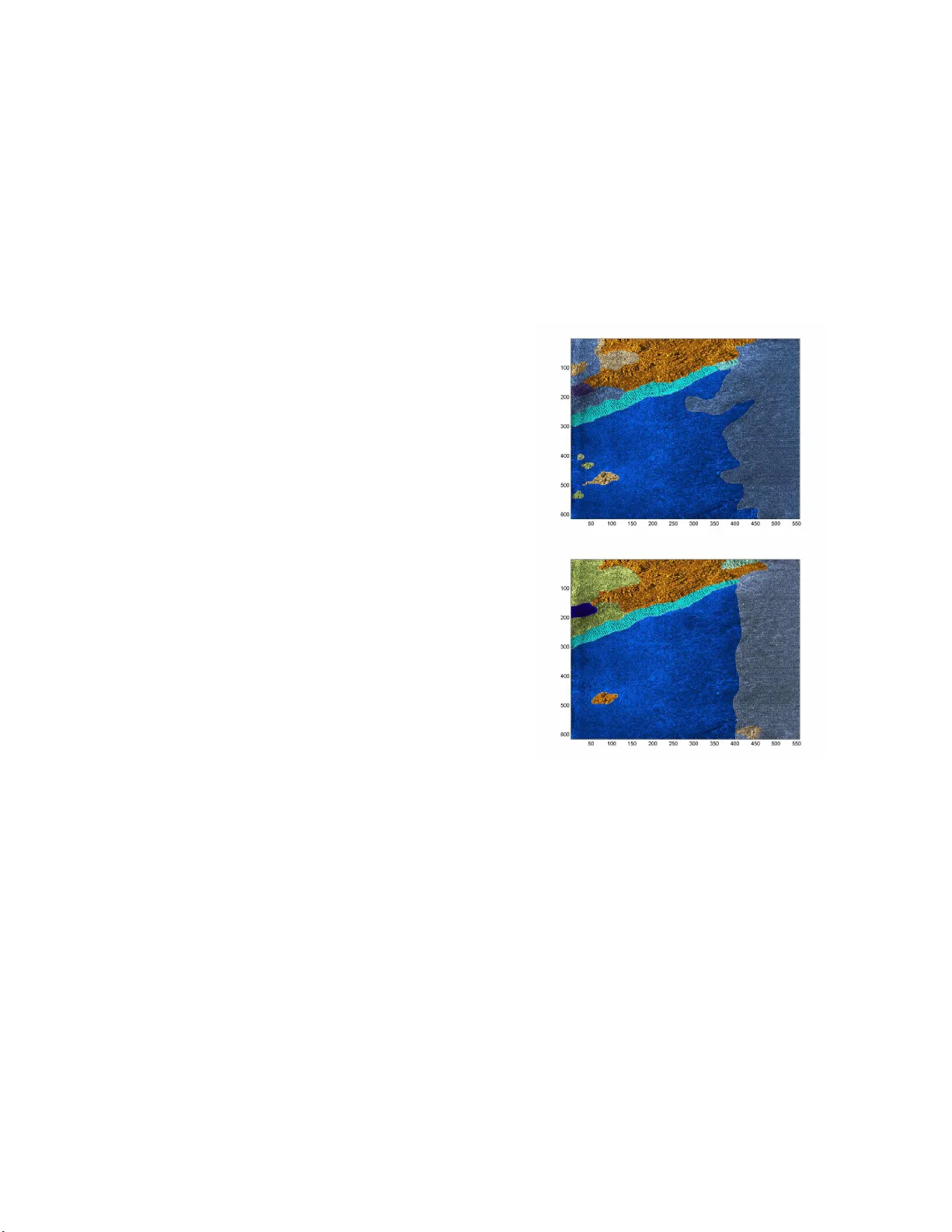
Decision Support with Belie f F unctions Theory for Seabed Characte rizati on Arnaud Martin ENSIET A, E 3 I 2 - EA38 76 2, rue Franc ¸ ois V erny 29806 Brest, Cedex 9, Fra nce Email: Arn aud.Martin @ensieta.fr Isabelle Quidu ENSIET A, E 3 I 2 - EA38 76 2, rue Franc ¸ ois V erny 29806 Brest, Cedex 9, Fra nce Email: Isabelle.Quid u@ensieta.fr Abstract — The seabed characterization from sonar images is a very hard ta sk because of the pro duced data and the unknown en viro nment, e ven for an human expert. In this work we propose an original approach in order to combine binary classifiers arising from different kinds of strategies such as one-versus- one or on e-versus-r est, usu ally used in the SVM-classification. The decision fu nctions coming from th ese bi nary classifiers are interpreted in terms of bel ief functions in order to combine these functions with one of th e nu merous op erators of th e belief functions theory . Moreo ver , th is int erpr etation of the decision function allows us to propose a process of decisions by taki ng into account the rejected observations too far remo ved from the learning data, and the imprecise d ecisions given i n un ions of classes. This new approac h is illustrated and ev aluated with a SVM in order to classify th e di fferent kinds of sediment on image sonar . Keywords: belief functions t heory , decision support, SVM, sonar image. I . I N T RO D U C T I O N Sonar images are obtained from temporal measurements made by a lateral, or frontal sonar trailed by the back of a boat. Each emitted signa l is reflected on the b ottom then received on the antenna of the sonar with an adjustable delay ed in tensity . Receiv ed data are very noisy . T here are some interfer ences due to the signal travelling on multiple p aths (r eflection on th e bottom or surface), due to spe ckle, and due to fauna and flora . Therefo re, sonar images are chraracter ized by im precision and u ncertainty ; thus sonar im age classification is a d ifficult problem [1]. Figure 1 shows the differences between the interpretatio n an d the certainty of two sonar experts trying to differentiate typ es of sediment (ro ck, cob bles, sand, ripple, silt) or shadow when the info rmation is invisible (e ach color correspo nds to a kind of sediment and the a ssociated certainty of the expert is exp ressed in terms of sur e, moderate ly sure and not sure ) [ 2]. The autom atic classification appro aches, fo r sonar imag es, are based on texture analysis and a classifier such as a SVM [3]. The su pport vector m achines ( SVM) is b ased on an optimization appro ach in order to separate two classes b y an h yperplan e. For p attern reco gnition with se veral classes, this optimiza tion ap proach is po ssible (see [4]) but time con- suming. Hence a p referab le solution is to co mbine the b inary classifiers according to a classical strategy such as one- versus- one or one-versus-rest. The co mbination of these classifiers Fig. 1. Segme ntatio n giv en by two expert s . is gener ally formed with very simple approach es such as a voting rule or a maxim ization of decision functio n co ming from the classifiers. Ho wever , many combination operato rs can be u sed, especially in the belief f unction s framework ( cf. [5]) . Belief fu nctions theory h as bee n already em ployed in ord er to combine the b inary classifier origina lly from SVM (see [6 ], [7]). The op erators in the belief function s the ory d eal with the conflict a rising from the binary c lassifiers. Another interest of this theory is that we can ob tain a b elief d egree o n the unions of classes and not only o n exclu si ve classes. Ind eed the decisions of the bin ary classifiers can be difficult to take when data overlap. From the decision func tion, we can define probab ilities in order to combin e them ( cf. [ 8]). Howe ver , a probab ility measure is an additive measure and so prob abilities cannot easily pr ovide a decision on unions of classes unlike belief func tions. Hence, onc e the binary cla ssifiers have been combin ed, we propo se belief functions in or der to take the decision fo r one class only if this class is credible enou gh, for the unio n of two or more classes oth erwise. Moreover , accor ding to th e application it could be in teresting to not take the decision o n one of the learning c lasses, and reject data too far from the learning classes. Many classical appr oaches are possible in pattern recog nition fo r outliers rejection (see [ 9], [10]) . W e propo se here to in tegrate ou tliers r ejection in our decision process based on b elief functio ns. In additio n to this n ew decision pro cess, th e originality of the p aper co ncerns th e mo delization that we p ropose, i.e. how to define t he belief functions, on the basis of decision functions coming from th e binary classifiers. This pap er is organize d as follows: in section II we recall the p rinciple o f th e sup port vector ma chines for classification. Next, we present the belief func tions theo ry in section III in order to pro pose in section IV o ur belief appro ach to com- bine the binary classifiers and to provide a decision proce ss allowing the o utliers r ejection and the indecision expr essed as possible decisions on unio ns. This approach is ev a luated for seabed charac terization on so nar images in section V. I I . S V M F O R C L A S S I FI C AT I O N Suppor t vector machin es were introdu ced by [11] based o n the statistical learning th eory . Hence, SVM can be used for estimation, regre ssion or pattern r ecognitio n like in this paper . A. Princ iple of the SV M The support vector machine appro ach is a binary c lassi- fication method . It classifies positive and negative p atterns by sear ching the op timal hy perplan e th at separa tes th e two classes, while g uaranteein g a max imum d istance between the nearest p ositiv e and n egati ve p atterns. T he h yperplan e that maximizes this distance called mar gin is determin ed by pa r- ticular p atterns called support vectors situated at the b ounds of the margin. These only fe w supp ort vector number s are used to classify a ne w pattern, which makes SVM v ery f a st. The po wer of SVM is also due to th eir simplicity o f imp lementation and to solid theo retical bases. If the p atterns are linearly separa ble, we search the hyper- plane y = w .x + b wh ich max imizes th e margin between the two classes where w .x is the d ot prod uct of w and x , and b the bias. Thus w is the solutio n of the conve x optimization problem : Min k w k 2 / 2 (1) subject to: y t ( w.x t + b ) − 1 ≥ 0 ∀ t = 1 , . . . , l , (2) where x t ∈ I R d stands for o ne o f the l learning data, and y t ∈ {− 1 , +1 } the associated class. W e can solve this optimization pro blem with th e following L agrang ian: L = k w k 2 2 l X t =1 Λ t ( y t ( w.x t − b ) − 1) , (3) where the Λ t ≥ 0 are the Lagrang e multipliers, satisfying l X t =1 Λ t y t = 0 . If th e d ata are n ot linearly separable, th e co nstraints ( 2) are relaxed with the intr oduction o f p ositiv e terms ξ t . In this case we search to min imize: 1 2 k w k 2 + C l X t =1 ξ t , (4) with the con straints given f or all t :  y t ( w.x t + b ) ≥ 1 − ξ t ξ t ≥ 0 (5) where C is a co nstant given by the user in order to weig ht the error . This pro blem is solved in the same way as the lin ear separable case with Lagrange mu ltipliers 0 ≤ Λ t ≤ C . T o classify a new pattern x we simp ly need to stud y the sign of the d ecision fun ction given by : f ( x ) = X t ∈ S V y t Λ t x t .x − b, (6) where S V = { t ; Λ t > 0 } fo r the separab le c ase and S V = { t ; 0 < Λ t < C } fo r the non-sep arable c ase, is the set of ind ices of th e suppor t vectors, and Λ t are the Lagr ange multipliers. In the no nlinear cases, the comm on idea of the kern el approa ches is to map the data in a high dimension. T o do that we use a kerne l function th at mu st be bilinear, sym metric and positi ve and correspon ds to a dot pro duct in the ne w space. The classification of a n ew pattern x is giv en by the sign of the decision fun ction: f ( x ) = X t ∈ S V y t Λ t K ( x, x t ) − b (7) where K is the kernel func tion. Th e most used kern els ar e th e polyno mial K ( x, x t ) = ( x.x t + 1) δ , δ ∈ I N, and th e radial basis fu nctions K ( x, x t ) = e − γ k x − x t k 2 , γ ∈ I R + . The choice of the kernel is not always ea sy and generally left to the user . B. Multi-c lass cla ssification with SV M W e can distinguish two kinds of approaches in or der to use SVM fo r classification with n classes, n > 2 . The first one c onsists in fusing se veral binary classifiers given by the SVM - the obtain ed results by each classifier are comb ined to produ ce a fina l result following strategies suc h as one -versus- one or one-versu s-rest. The seco nd on e con sists in considerin g the optimization pro blem. • Dir ect approac h: in [4], the notio n o f margin is extended to the m ulti-class p roblem. Howe ver, this appro ach be- comes very time consum ing, espe cially in the no nlinear case. • o ne-versus-rest: Th is approach con sists in learning n de- cision fun ctions f i , i = 1 , ..., n given by the equation s (6) or (7) accordin g to the c ases, allowing the d iscrimination of ea ch class from th e n − 1 others. The a ffection of a class w k to a new p attern x is generally given by the relation : k = a r g max i =1 ,...,n f i ( x ) . I n the non linear case, we ha ve to be caref ul of the p arameters of the kernel function s that could have some different o rders f ollowing the learn ing binary classifiers. So, it cou ld be better to decide on normalized functions calculated f rom the decision fun ctions (see [1 2], [13 ]). • o ne-versus-on e: In stead of learning n decision fun ctions, we tr y here to discriminate each class from each o ther . Hence we hav e to learn n ( n − 1) / 2 decision fun ctions, still given by eq uations ( 6) or (7) according to th e different ca ses. Each decision fun ction is considered as a vote in o rder to classify a new pattern x . The class of x is given by the ma jority voting ru le. Some oth er methods have b een propo sed b ased on pr evious ones: • Err o r -Corr ecting Output Codes (ECOC): let w i , i = 1 , ..., n , be the classes, S j , j = 1 , ..., s , th e different classifiers ( s = n in the case one -versus-rest and s = n ( n − 1) / 2 in the ca se one-versus-one) , ( M ij ) , the matr ix of the codes with the classes in row and th e classifiers in colu mn, stands for the contribution of each classifier to the final resu lt o f the classification (b ased on the error of all the classifiers). The final decision is giv en co mparing the results of the classifiers with each row of the matrix ; the class of a new p attern x is the class giving the least e rror (see [14 ]). • Acc ording to the decision functions, [8] d efined a pro b- ability (1 9) in ord er to nor malize the decision fun c- tions. Hence, we can com bine th e b inary classifiers (for both one-versus-rest an d one-versus-one cases) with a Bayesian rule (see [15]) or with more simple rules (see [7]). • DA GSVM (Dire cted Acyclic Graph SVM) propo sed by [16]: In this approach , the learning is made as the one- versus-one w ith the learning of n ( n − 1) / 2 binary decision function s. In or der to gen eralize, a binary decision tre e is considered wh ere each node stands for a binary classifier and each leaf stands for a class. Eac h b inary classifier eliminates a class and the class of a new pattern is the class given by the last n ode. I I I . B E L I E F F U N C T I O N S T H E O RY The belief functions theory , also ca lled e v idence theory o r Dempster-Shafer theor y (see [17], [18]) is more a nd more employed in ord er to take into acco unt the uncertain ties and impr ecisions in p attern recog nition. The belief functions framework is b ased on th e use o f functio ns d efined on the p ower set 2 Θ (the set of all th e subsets of Θ ), wh ere Θ = { w 1 , . . . , w n } is the set of exclusi ve and exha ustiv e classes. These belief functions or ba sic b elief a ssignments , m j are defined by the mapping of the power set 2 Θ onto [0 , 1] with generally: m j ( ∅ ) = 0 , (8) and X X ∈ 2 Θ m j ( X ) = 1 , (9) where m j ( . ) is th e b asic b elief assign ments for a n exper t (or a binary classifier) S j , j = 1 , ..., s . Thus in the one -versus-rest case s = n and in the o ne-versus-on e case s = n ( n − 1) / 2 . The eq uation (8) makes the assump tion of a closed world (that m eans that all the classes are exhaustive) [18 ]. W e can define the belief fu nctions only with: m j ( ∅ ) ≥ 0 , (10) and the world is open ( cf. [19 ]). But in order to chang e an open world to a clo sed world, we can add o ne element in the discriminating space and th is elemen t can b e con sidered as th e garbag e class. T he difficulty , as we will see later, is the mass that we have to allocate to this elem ent. W e have two ad vantages with the belief fun ctions theo ry compare d to the p robabilities and Bay esian approaches. Th e first one is the possibility for one expert ( i.e. a b inary classifier) to de cide that a new patter n belong s to the union of some classes without needing to d ecide an u nique class. The basic belief function s are not ad ditiv e that gives more freed om f or the mo delization of som e pr oblems. Th e second o ne is the modelization o f som e pr oblems witho ut any a priori b y g iving the mass of belief on the ignorance s ( i.e. the unions of class es). These simp le co nditions in eq uations (8) and (9), give a large panel of definition s of the belief fun ctions, which is on e of the difficulties of the theory . From the se basic belief assignmen ts, other belief f unctions can b e defined such as credib ility a nd plausibility . The cred ibility r epresents the intensity that the infor mation g i ven by on e exper t supp orts an element of 2 Θ , this is a minimal belief function given fo r all X ∈ 2 Θ by: bel( X ) = X Y ⊆ X, Y 6 = ∅ m j ( Y ) . (11) The p lausibility r epresents th e in tensity with which th ere is n o doubt on one element. This function is given for all X ∈ 2 Θ by: pl( X ) = X Y ∈ 2 Θ ,Y ∩ X 6 = ∅ m j ( Y ) = b el(Θ) − b el( X c ) = 1 − m j ( ∅ ) − bel ( X c ) , (12) where X c is the co mplementar y o f X in Θ . T o keep a maximum o f in formation , it is p referab le to combine inform ation g iv e n by the basic belief assignments into a new b asic belief assignment an d take the decision on one o f the obtaine d belief fun ctions. Many co mbinatio n rules have been proposed . The con junctive rule p ropo sed by [2 0] allows us to stay in an open world. It is define d for s expe rts, and for X ∈ 2 Θ by: m Conj ( X ) = X Y 1 ∩ ... ∩ Y s = X s Y j =1 m j ( Y j ) , (13) where Y j ∈ 2 Θ is the re sponse o f the expert j , and m j ( Y j ) the cor respond ing basic b elief assignment. Initially , [ 17] and [18] ha ve p roposed a conjunctive nor- malized rule, in order to stay in a closed world. This rule is defined for s c lassifiers, fo r all X ∈ 2 Θ , X 6 = ∅ b y: m DS ( X ) = 1 1 − m Conj ( ∅ ) X Y 1 ∩ ... ∩ Y s = X s Y j =1 m j ( Y j ) = m Conj ( X ) 1 − m Conj ( ∅ ) , (14) where Y j ∈ 2 Θ is th e resp onse of the expert j , and m j ( Y j ) the correspo nding b asic belief assignment. m Conj ( ∅ ) is generally interpreted as a con flict mea sure or more exactly as the inconsistence of the fusion - b ecause of the n onidem potence of the r ule. This r ule applied o n basic b elief assignments where the only focal elemen ts are the classes w j ( i.e. some probab ilities) is equiv alent to a Bayesian appr oach. A shor t revie w of all th e combination rules in the belief functions framework and a nu mber of new rule s are given in [5] . If the cred ibility functio n provides a p essimistic decision , the plau sibility fun ction is often too optimistic. T he pig nistic probab ility [1 9] is ge nerally consider ed as a comp romise. I t is calculated from a basic belief assignm ent m for all X ∈ 2 Θ , with X 6 = ∅ b y: betP ( X ) = X Y ∈ 2 Θ ,Y 6 = ∅ | X ∩ Y | | Y | m ( Y ) 1 − m ( ∅ ) , (15) where | X | is the cardinality of X . In this p aper, we wish to reject p art of the data that we do not consid er in the learning classes. Hence a p essimistic decision as to the maximum of the credibility fun ction is preferab le. An other criterion proposed by [21 ], consists in attributing the class w k for a new pattern x if: ( bel ( w k )( x ) = max 1 ≤ i ≤ n bel ( w i )( x ) , bel ( w k )( x ) ≥ b el ( w c k )( x ) . (16) The additio n of this seco nd condition on the m aximum of credibility , allows a decision on ly if it is nonamb iguou s, i.e. if we believe more in the class w k than in the subset of the other classes (the co mplemen tary of the class). Another approach proposed in [22] considers the plausibility function s and giv es the possibility to decide whichever elemen t of 2 Θ and no t on ly the sin gletons as previously . T hus the new pattern x belo ngs to the elemen t A of 2 Θ if: A = ar g max X ∈ 2 Θ ( m b ( X )( x )pl( X )( x )) , (17) where m b is a basic be lief assignment given by: m b ( X ) = K b λ X  1 | X | r  , (18) r is a parameter in [0 , 1] allowing a decision from a simple class ( r = 1 ) until the total indecision Θ ( r = 0 ) . λ X allows the integration of the lack of knowl edge on one of the elements X in 2 Θ . I n this pap er , we will chose λ X = 1 . T he co nstant K b is the normalization factor giving by the con dition of the equation (9). I V . B E L I E F F U N C T I O N S T H E O RY F O R C L A S S I FI C A T I O N W I T H S U P P O RT V E C T O R M A C H I N E S In the previous sections, we hav e described the two main strategies in ord er to build a multi-class classifier fro m b inary classifiers: th e on e-versus-rest and o ne-versus-on e approaches. Most of the time the formalism to combine the binary class ifier results is different accord ing to the strategy . [23] have pro- posed a combination approach o f the binary classifier decisions based on the belief functions theory gi ven an unique formalism for both one- versus-one and o ne-versus-rest strategies. The basic belief assignmen ts are d efined f rom con fusion matrice s of th e binary classifiers. W orking directly on the classifier decisions allows a lo ss of informa tion contained first in the decision function s. Thus it cou ld be b etter to defin e the basic belief assignments fr om the decision f unctions rather tha n from the confusion ma trices ( i.e. form th e classifier d ecisions). Howe ver, the decision fu nctions are not norma lized, so we can h ave pro blems in the combination of this function especially with the one-versus-rest strategy . [8] has d efined a probab ility from the se de cision functio ns f such as: P ( y = 1 / f ) = 1 1 + exp( Af + B ) , (19) where A and B are calculated in order to get P ( y = 1 / f = 0) = 0 . 5 . Different app roaches h av e been proposed for the estimation of these parameters (see [24]). [7] uses a one class SVM, introduced by [25]. So the combinatio n can be d one on ly with a on e-versus-rest strategy . The d ecision f unctions coming fro m this particular classifier are employed to define some p lausibility functio ns on the singleton w i : pl( w i )( x ) = f i ( x ) + ρ ρ , (20) where f i ( x ) is the decision function giving the distanc e b e- tween x and the fronter of class w i and ρ is a factor e stimated in the one-SVM algorithm that depend s on the kernel ( cf. [ 25]). The first origin ality of this pap er resides in the definition of the basic belief assignmen ts th at we obtain directly fro m the d ecision f unctions f given b y th e equ ations (6) o r ( 7). The basic idea con sists in con sidering the d ata dispe rsion in one of the semi-spaces given by the hy perplan e, f ollowing an exponential distribution. This distribution gives a dispersion of the d ata arou nd the mean mo re or less nea r to the h yperplan e, with the o pportu nity to ob serve data very far away from the hyperp lane. D oing this we keep the basic idea of the SVM. Hence, a ccording to the sign of the decisio n fu nction ( i.e. the semi-space de fined by the hyperp lane), the belief can b e ob tained by the cumulative density functio n of the exponential d istribution (see fig ure 2). W e define the basic belief assignmen t b y:                            m i ( w i )( x ) = α i  (1 − 1 2 exp( − 1 λ i,p f i ( x ))) 1 l [0 , + ∞ [ ( f i ( x )) exp( − 1 λ i,n f i ( x )) 1 l ] −∞ , 0[ ( f i ( x ))  m i ( w c i )( x ) = α i  exp( − 1 λ i,p f i ( x )) 1 l [0 , + ∞ [ ( f i ( x )) (1 − 1 2 exp( − 1 λ i,n f i ( x ))) 1 l ] −∞ , 0( ( f i ( x ))  m i (Θ)( x ) = 1 − α i where α i is a discountin g factor of the basic belief assignment, λ i,p and λ i,n are some p arameters depend ing on the decision function s of class w i that we defin e in equation (2 1). Th e ratio 1 2 is in troduce d to increase the belief to the c lass related to the semi-space wh ere the data ar e loc ated ( see figur e 2). There are many w ays to choose or to calculate the d iscounting factor that is generally clo se to one. [26] propo ses a method to obtain the discounting factor that optimizes the decision taking advantage of the p ignistic prob ability . W e prop ose her e to calculate th is discounting factor acco rding to the good classification r ate of binary classifiers. The g ood classification rates are calculated with the study of the sign of the d ecision function f i on the learning data used to determin e the model of binar y classifiers. Fig. 2. Illustra tion of the basic belief assignment based on the cumulati ve density function of the exponent ial distributi on. W e propo se to e stimate the λ i parameters from the mean of th e decision functions on the learning data in ord er to b e coheren t with the exponential distrib u tion. Hence λ i,p and λ i,n are given by:            λ i,p = 1 l l X t =1 f i ( x ) 1 l [0 , + ∞ [ ( f i ( x )) , λ i,n = 1 l l X t =1 f i ( x ) 1 l ] −∞ , 0[ ( f i ( x )) . (21) This prop osed basic belief assignment mod el allows a goo d modelization of the info rmation g iv e n b y th e binary classifiers in o rder to combine them by both one-versus-rest and on e- versus-one strategies. Thus for a one-versus-r est strategy , w c i represents the union of the other classes than w i , i.e. Θ r { w i } . In the on e-versus-one ca se, the d ecision func tions f i , i = 1 , ..., n ( n − 1 ) / 2 can be re w ritten as f ij with i < j and i, j = 1 , ..., n , where i a nd j corr espond to the considered classes w i and w j . In this one- versus-one case, w c i must be seen as w j and the b asic b elief assignment ar e g iv e n by:                            m ij ( w i )( x ) = α ij  (1 − exp( − 1 λ ij,p f ij ( x ))) 1 l [0 , + ∞ [ ( f ij ( x )) + exp( − 1 λ ij,n f ij ( x )) 1 l ] −∞ , 0[ ( f ij ( x ))  m ij ( w j )( x ) = α ij  exp( − 1 λ ij,p f ij ( x ))) 1 l [0 , + ∞ [ ( f ij ( x )) (1 − exp( − 1 λ ij,n f ij ( x ))) 1 l ] −∞ , 0[ ( f ij ( x ))  m ij (Θ)( x ) =1 − α ij with            λ ij,p = 1 l l X t =1 f ij ( x ) 1 l [0 , + ∞ [ ( f ij ( x )) , λ ij,n = 1 l l X t =1 f ij ( x ) 1 l ] −∞ , 0[ ( f ij ( x )) . (22) W e use here the conjunctive norma lized rule (equation (14)). Thus we can apply this rule in order to combine the n basic b elief assignme nts in the one-versus-rest case an d the n ( n − 1) / 2 ba sic belief assign ments in the one-versus-one case. When the data overlap a lot, mo re complicated rules such as pro posed in [5] cou ld be prefer red. For the d ecision step, we want to keep the p ossibility to take the d ecision o n a union of classes ( i.e. when we can no t decide between two par ticular classes) and also to no t take a decision wh en ou r b elief in one foca l element is to o we ak. Thus we pr opose the following dec ision rule in two steps: 1) Th e decision rule of the maximum of the credibility with reject defined b y the e quation (16) is ap plied in ord er to determine the patterns that d o not belong to the learn ing classes. 2) Th e decision rule g i ven by the eq uation (17) is next applied to the n on-rejected patterns. Another possible decision proc ess could be first the appli- cation of the decision r ule given b y the equation (17), an d next the decision ru le of the maximu m of the credibility with reject on the imprecise pa tterns that first belo ng to the union s of classes. On the illustrated d ata given in the next section, we obtain similar results. W e call this decision process (2-1) and the previous o ne (1-2 ). V . A P P L I C A T I O N A. So nar d ata Our database con tains 42 sonar images provided by the GESMA (Gr oupe d’ Etudes Sous-Ma rines de l’Atlantiqu e). These images were obtained with a Klein 5400 later al sonar with a r esolution o f 20 to 30 c m in azim uth and 3 cm in range . The sea-botto m dep th was b etween 1 5 m an d 40 m. Some experts hav e manually segmented these images giving the kind of sediment (rock, cobble, sand, silt, ripple (vertical or at 45 degrees)), shadow o r other (typically shipwrecks) parts on images. It is very d ifficult to discrim inate the rock and the the co bble an d also the san d and silt. However , it is importa nt for the sedimentologists to discriminate the sand and the silt. The type “ ripple” can be some ripple of san d or ripple o f silt. Hence, with the point of view o f th e sedimentolo gists we consider only th e three classes of sedim ent: C 1 =rock-c obble, C 2 =sand an d C 3 =silt. An d in order to ev alu ate ou r decision process, we take the ripple as the fourth c lass ( C 4 ) that is unlearne d. Each image is cut o ff in tiles of size 32 × 32 p ixels (about 6.5 meter b y 6.5 meter). W ith th ese tiles, we keep 35 00 tiles of each class with only on e k ind o f sedime nt in the tile. Hence, our database is made of 4 × 35 00 tiles. W e con sider 2/3 of them for the learning step (on ly for the th ree classes of sediment) and 1/3 of them f or the test step ( i.e. 1167 tiles for each kind of sediment) . In order to classify the tiles of size 32 × 32 pixels, we first hav e to extract texture p arameters from each tile. Here, we cho ose th e co-occu rrence ma trices app roach [1]. The co- occurre nce matrices are calculate d by number ing the o ccur- rences of identical gray level of two p ixels. Six par ameters giv en by Hara lick are ca lculated: hom ogeneity , co ntrast esti- mation, entropy estimatio n, th e c orrelation , the d irectivity , an d the unifo rmity . Concer ning th ese six param eters, we calculate their m ean o n four direction s: 0, 45, 90 and 1 35 degrees. The prob lem for co-occur rence m atrices is the n on-inv ar iance in translation. T y pically , this problem can appear in a ripp le texture character ization. More features extraction ap proach es can be u sed such as the run- lengths matrix, the wa velet transform and th e Ga bor filters [1 ]. W e use the libSVM [2 7], and after comparin g several ker- nels, we have r etained the radial basis function (with γ = 1 / 6 where 6 is the dimen sion of the data) and we take weighting of the er ror C = 1 bec ause of the data overlap. B. Resu lts The table I shows th e results for the SVM classifier with the strategies one-versu s-one and one-versus-re st. W e note tha t there are many er rors between the sand ( C 2 ) and silt ( C 3 ), that are two homog eneous sediments. The r ipple ( C 4 ), the unlearnin g class, is more hetero geneo us than the sand a nd silt, this why it is more classified as ro ck ( C 1 ). Th e table II one-vs-one one-vs-rest % C 1 C 2 C 3 C 1 C 2 C 3 C 1 91.00 8.83 0.17 84.40 15.08 0.51 C 2 7.11 80.72 12.17 2.57 61.27 36.16 C 3 2.06 30.42 67.52 0.86 22.71 76.44 C 4 65.13 33.16 1.71 52.36 45.41 2.21 T ABLE I R E S U LT S O F T H E S V M C L A S S I F I E R F O R T H E B O T H S T R ATE G I E S O N E - V E R S U S - O N E A N D O N E - V E R S U S - R E S T . shows the same results, but with the pro posed app roach based on the belief function th eory (pr esented in section III) with the dec ision based on the p ignistic p robability . This ap proach provides some similar results than the basic version s of the SVM (table I). N ote th at the strategy one-versus-rest provid es more erro rs between the sand and silt. This can be explained because the da ta overlap. In the rest of th e paper we consider only the on e-versus-one strategy . one-vs-one one-v s-rest % C 1 C 2 C 3 C 1 C 2 C 3 C 1 88.00 11.91 0.09 91.51 6.18 2.31 C 2 4.80 83.29 11.91 8.83 20.90 70.27 C 3 1.20 32.05 66.75 2.06 5.23 92.71 C 4 56.38 41.99 1.63 67.52 20.57 1 1.91 T ABLE II R E S U LT S O F T H E S V M C L A S S I FI E R W I T H B E L I E F F U N C T I O N T H E O RY F O R T H E B O T H S T R A T E G I E S O N E - V E R S U S - O N E A N D O N E - V E R S U S - R E S T . The table II I giv es th e results with p ossible decision on unions with r = 0 . 6 . W e can see tha t this k ind of cautio us decision provid es less har d err ors ( i.e. say one kind of sed i- ment instead of another). Of course these results depend on the values of r th at pr ovide a mo re or less cau tious decision as we can see on figure 3. If we a dd the possibility o f rejection to these resu lts (ta ble IV) , we can see that the m ost o f r ejected tiles come f rom the rip ple (the u nknown class C 4 ). For a given class, the rejected tiles co me as a major ity from the unions (imprecise data). Of cou rse this r ejection does not dep end o n the r value if we begin b y the rejection in o ur decision process (1-2) (presen ted in section III). Figure 3 shows the results of the classification of class of ripple ( C 4 ) accord ing to the value of r without possible rejection. Of co urse when the value o f r is weak the data of the th ree learning classes are classified on the unions. W e can distinguished three kin ds of work intervals o n these data: • r ∈ [0; 0 . 3] : The classifier is to o und ecided, • r ∈ [0 . 4; 0 . 6 ] : the amb iguity betwe en the classes is correctly consider ed, • r ∈ [0 . 7; 1] : the decision is too hard. Fig. 3. Classification of the class of ripple ( C 4 ) with possible decision on union according to r . According to the ap plication, if we want to privilege the hard decision at the expense of the rejection, we can try to % C 1 C 2 C 3 C 1 ∪ C 2 C 1 ∪ C 3 C 2 ∪ C 3 C 1 ∪ C 2 ∪ C 3 C 1 76.69 6.86 0 15.68 0 0.77 0 C 2 0.86 50.04 4.97 11.83 0 32.30 0 C 3 0.35 17.05 53.21 2.14 0 27.25 0 C 4 38.99 22.62 1.12 33.16 0 4.11 0 T ABLE III R E S U LT S W I T H A B E L I E F C O M B I N AT I O N W I T H P O S S I B L E D E C I S I O N O N U N I O N S . % C 1 C 2 C 3 C 1 ∪ C 2 C 1 ∪ C 3 C 2 ∪ C 3 C 1 ∪ C 2 ∪ C 3 C 4 C 1 76.69 6.26 0 6.34 0 0.34 0 10.37 C 2 0.86 48.93 4.97 1.63 0 19.45 0 24.16 C 3 0.34 15.42 53.22 0.34 0 12.77 0 17.91 C 4 38.99 20.65 1.11 9.68 0 1.63 1.71 27.93 T ABLE IV R E S U LT S W I T H A B E L I E F C O M B I N AT I O N W I T H P O S S I B L E D E C I S I O N O N U N I O N S A N D O N T H E R E J E C T E D C L A S S . decide first, possibly on th e unions and next try to reject o nly on th e unio ns. In this case we can choose a higher value o f r . For example with r = 0 . 8 , we propo se a comparison o f the dec ision pr ocesses (1-2) with (2-1) g i ven in the table V. Of course the decision process (2-1 ) rejects less data, but it is only with the rock (class C 1 ) that we win, and we reject less ripple ( class un known C 4 ). Hence, it seems that the decision process (1-2 ) is b etter for this ap plication. Now let’ s co nsider th e tiles con taining mor e than two kinds of sedim ent. W e still lear n the SVM classifier with the same p arameter a nd th e one-versus-one strategy on the homog eneous tiles of the three classes rock ( C 1 ), sand ( C 2 ) and silt ( C 3 ) as previously . For th e tests, we only take 299 tiles with the classes: S 1 =tiles with ro ck an d sand , S 2 =sand and silt, S 3 =silt and ripple and S 4 =sand and rip ple. T able VI presen ts th e obtain ed r esults of the SVM classifier with the classical voting c ombinatio n and a b elief combina- tion with pig nistic decision and with cred ibility with reject decision. For th e two classes S 1 and S 2 , the tiles c ontain o nly learning sediment ( rock and sand f or S 1 and sand an d silt for S 2 ). For S 1 and S 2 the cla ssifiers witho ut reject classify these tiles more in sand. The rejection decreases the errors, but for S 2 the r ejection is essentially o n the sand. T he two classes S 3 and S 4 contain rip ple, the unk nown class. Here also, we no te a con fusion with the rock sed iment that is an heterogen eous texture like the r ipple. The rejection for the se two classes works well, b ecause a large part of the tiles classified in rock are rejected and for S 3 a large pa rt of tiles classified in san d are also rejected . T able VII shows the results with possible decision on th e union with r = 0 . 6 , with and withou t possible rejection. The addition of the possible de cision on the union red uces the errors. The rejection is e ssentially on the tiles classified on the unio ns, except for S 2 (sand and silt) a lot o f classified- sand tiles ar e r ejected, may be bec ause of the lear ning step. Hence, for the tiles containin g more than on e kind of sediments our decision support could help the human experts. Of co urse, in th is ca se, the ev alu ation is really difficult. In [2] we hav e propose co nfusion matrices taking into acco unt the propo rtion of each sediment in a tile. V I . C O N C L U S I O N S W e have propo sed an or iginal approach based on the belief function s th eory for th e combinatio n of binar y classifiers coming from the SVM with o ne-versus-on e or one- versus-rest strategies. The mo delization o f the basic belief assignmen ts is pr oposed d irectly from th e decision f unctions given by the SVM. T hese basic belief assignments allow to take correctly into account th e principle of th e binary classifi cation with SVM b y comparison with an hy perplan e in line ar or n onlinear cases. The belief f unction s theory provides a decision supp ort without n ecessary de ciding an exclusiv e class. The decision process that we have p roposed with possible outliers re jection and with p ossible decision o n the union of classes, is very interesting because it works like the intuiti ve classification that a h uman could p erform based on the position o f supp ort vectors a nd considering the ambiguity o f the classes. This deci- sion support can really help experts for seabed characterization from sonar ima ges. W e have seen with th e point o f v iew of the sedimentolo gists that if we only consider th e dif f erent kind s of sedim ents (rock, sand and silt), the amb iguity between the sand and the silt is well recognize and th e ripple can be partly rejected. vote pignisti c with reject % C 1 C 2 C 3 C 1 C 2 C 3 C 1 C 2 C 3 C 4 S 1 27 . 4 67 . 2 5 . 4 20 . 4 74 . 9 4 . 6 15 . 4 56 . 5 3 . 3 24 . 8 S 2 1 . 3 40 . 5 58 . 2 0 . 3 44 . 8 55 . 9 0 14 . 4 47 . 8 37 . 8 S 3 40 . 1 38 . 1 21 . 8 34 . 1 44 . 8 21 . 1 24 . 4 24 . 1 18 . 1 34 . 4 S 4 40 . 8 58 . 2 1 . 0 31 . 8 67 . 2 1 . 0 22 . 7 51 . 2 1 . 0 26 . 1 T ABLE VI R E S U LT S O F T H E S V M C L A S S I F I E R W I T H T H E C L A S S I C A L V O T I N G C O M B I N ATI O N A N D A B E L I E F C O M B I N ATI O N W I T H P I G N I S T I C D E C I S I O N A N D W I T H C R E D I B I L I T Y W I T H R E J E C T D E C I S I O N . % C 1 C 2 C 3 C 1 ∪ C 2 C 1 ∪ C 3 C 2 ∪ C 3 C 1 ∪ C 2 ∪ C 3 C 4 C 1 82.86 6.77 0 0 0 0 0 10.37 C 2 2.23 64.44 9.17 0 0 0 0 24.16 C 3 0.69 20.48 60.92 0 0 0 0 17.91 C 4 48.67 21.94 1.46 0 0 0 0 27.93 C 1 87.75 4.20 0 0.43 0 0 0 5.06 C 2 4.54 64.44 9.17 0.34 0 0 0 21.51 C 3 1.20 20.48 60.93 0.08 0 0 0 17.31 C 4 55.78 21.94 1.46 1.20 0 0 0 19.62 T ABLE V R E S U LT S W I T H A B E L I E F C O M B I NAT I O N W I T H P O S S I B L E D E C I S I O N O N U N I O N S A N D O N T H E R E J E C T E D C L A S S ( 1 - 2 ) A N D W I T H R E J E C T I O N O N T H E U N I O N O N LY ( 2 - 1 ) . % C 1 C 2 C 3 C 1 ∪ C 2 C 1 ∪ C 3 C 2 ∪ C 3 C 1 ∪ C 2 ∪ C 3 C 4 S 1 8.03 49.50 1.67 26.75 0 14.05 0 - S 2 0 23.08 37.46 3.34 0 36.12 0 - S 3 16.05 22.41 1 5.38 30.44 0 15.72 0 - S 4 15.72 47.49 0.33 31.44 0 5.02 0 - S 1 8.03 48.16 1.67 9.36 0 8.03 0 24.75 S 2 0 12.71 37.46 0 0 12.04 0 37.79 S 3 16.05 21.40 1 5.38 8.70 0 5.02 0 33.45 S 4 15.72 47.16 0.33 7.02 0 3.68 0 26.09 T ABLE VII R E S U LT S W I T H A B E L I E F C O M B I N AT I O N W I T H P O S S I B L E D E C I S I O N O N U N I O N S W I T H A N D W I T H O U T P O S S I B L E R E J E C T I O N . R E F E R E N C E S [1] A. Martin, “Compara ti ve study of information fusion methods for sonar images classifica tion, ” in The Eighth Internati onal Confer ence on Infor- mation Fusion, Philadelphia, USA , 25-29 July 2005. [2] A. Martin, “Fusion for Eva luati on of Image Classification in Uncertain En vironments, ” in The E ighth International Confer ence on Information Fusion, Florence , Italy , 10-13 July 2006. [3] H. Laanaya, A. Martin, D. Aboutajdine , and A. Khenchaf, “Kno wledge Discov ery on Database for Seabed Charact erizat ion, ” in Magr ebian Con- fer ence on Information T ech nolog ies, Agadir , Mor occo , 7-9 December 2006. [4] J. W eston and C. W atkins, “Support V ector Machines for Multi-Class Pat- tern Recognitio n Machine s, ” in CSD-TR-98-04, Department of Computer Scienc e, Royal Holloway , Universit y of London , 1998. [5] A. Martin and C. Osswald, “T ow ard a combination rule to deal with partia l conflict and specificit y in belief funct ions theory , ” in Internat ional Confer ence on Information Fusion , Qu ´ ebec, Canada, 2007. [6] A. Aregui and T . Denœux, “Fusion of one-class classifier in the belief functio n frame work, ” in International Conferen ce on Information F usion , Qu ´ ebec, Canada, 2007. [7] B. Quost and T . Denœux and M. Masson, “P airwise classifie r combination using belief functio ns, ” in P attern Recognitio n Lette rs , vol. 28, pp. 644– 653, 2007. [8] J. C. Platt, “Probabili ties for SV Machines, ” in Advances in Lar ge Margin Classifier s , ed. A.J. Sm ola, P . Barlett, B. Sch ¨ ol kopf and D. Schurmans, MIT Press, pp. 61–74, 1999. [9] C. Fr ´ elicot, “On unifing probabil istic/fuzzy and possibil istic rejec tion- based classifier from possibili stic clustered noisy data, ” in Advance in P attern Reco gnition, series Lectur e Notes in Computer Science , vol. 1451, pp. 736–745, 1998. [10] J. L iu and P . Gader , “Neural netw orks with enhanced outlie r rejecti on abili ty for off-line handwritt en word recognition, ” in P attern Recogni tion , vol. 35, no. 10, pp. 2061–2071, 2002. [11] V .N. V apnik, Statistical Learning Theory . John W esley and Sons, 1998. [12] J. Milgram and M. Cherier and R. Sabourin, “One-Against-One or One-Again st-All: Which O ne is Better for Hanwriting Recognitio n with SVMs?, ” in 10th Internationa l W orkshop on F ro ntier s in Handwri ting Recogn ition , La Baule, France, October 2006. [13] Y . Liu and Y .F . Zhen, “One-Against-All Multi-Class SVM Classificati on Using Reliabilit y Measures, ” in IEEE Internationa l J oint Confer ence on Neural Networks , vol. 2, pp. 849–854, 2005. [14] T .G. Dietteric h and G. Bakiri, “Solving Multiclass L earning Problems via Error-Correct ing Output Codes, ” in Jou rnal of Artificial Intellige nce Resear ch , vol. 2, pp. 263–286, 1995. [15] A. Lauberts and D. Lindgren, “Generali zation Ability of a Support V ector Classifier Applied to V ehicle Data in a Microphone Network, ” in Internati onal Confere nce on Information Fusion , Florence, Italia, 2006. [16] J.C. Platt and N. Cristiani ni and J. Shawe -T aylor , “Large Margin D AGs for Multic lass Classifica tion, ” in Advances in Neural Information Pr ocessing Systems , vol. 12, pp. 547–553, 2000. [17] A.P . Dempster , “Upper and Lo wer probabiliti es induced by a mul ti value d mapping, ” in Annals of Mathematic al Statistic s , vol. 38, pp. 325–339, 1967. [18] G. Shafer , A mathematical theory of evide nce . Princet on Univ ersity Press, 1976. [19] Ph. Smets, “Constructing the pignistic probabili ty function in a conte xt of uncertaint y , ” in Uncertainty in Artificial Intellige nce , vol. 5, pp. 29–39, 1990. [20] Ph. Smets, “The Combination of Evidence in the Transfer able Beli ef Model, ” in IE EE T ransactions on P attern Analysis and Machi ne Intelli - genc e , vol. 12, no. 5, pp. 447–458, 1990. [21] S. Le H ´ egarat -Mascle and I. Bloch and D. V idal-Mad jar , “ Applicat ion of Dempster-Shafer Evidence Theory to Unsupervised Classification in Multisourc e Remote Sensing, ” in IEE E T ransactions on Geoscience and Remote Sensing , vol. 35, no. 4, pp. 1018–1031, july 1997. [22] A. Appriou, “ Approche g ´ en ´ erique de la gestion de l’incertai n dans les processus de fusion multisenseur , ” in T raite ment du Signal , vol . 22, no 4, pp. 307–319, 2005. [23] H. Laanaya and A. Martin and D. Aboutajdin e and A. Khenchaf, “Seabe d classificati on using belie f multi-cl ass support vecto r machines, ” in Marine Env ironme nt Characterizat ion , Brest, France, octobe r 2006. [24] H.T . L in and C.-J. Lin and C. W eng, “ A Note on Platt’ s Probabilist ic Output for Support V ector Machines, ” in Machine Learning , 2008. [25] B. Sch ¨ ol kopf and J.C. Platt and J. Shawe-T aylor and A.J. Smola, “Es- timatin g the Support of a High-Dimensiona l Distrib ution, ” in Micr osoft Resear ch , 1999. [26] Z. Elouedi and K. Mellouli and Ph. Sm ets, “ Assessing Sensor Reliabil ity for Mult isensor Data Fusion Within The Transfe rable Belief Model, ” in IEE E T ransactions on Systems, Man, and Cybernetics - P art B: Cybernet ics , vol. 34, no. 1, pp. 782–787, 2004. [27] C.C. C hang and C.J. Lin, “Softwa re av ailab le at http:/ /www .csie.ntu.edu.tw/ ∼ cjlin/libsvm/ , ” in LIBSVM: a libr ary for support vector machines , 2001.