Fusion for Evaluation of Image Classification in Uncertain Environments

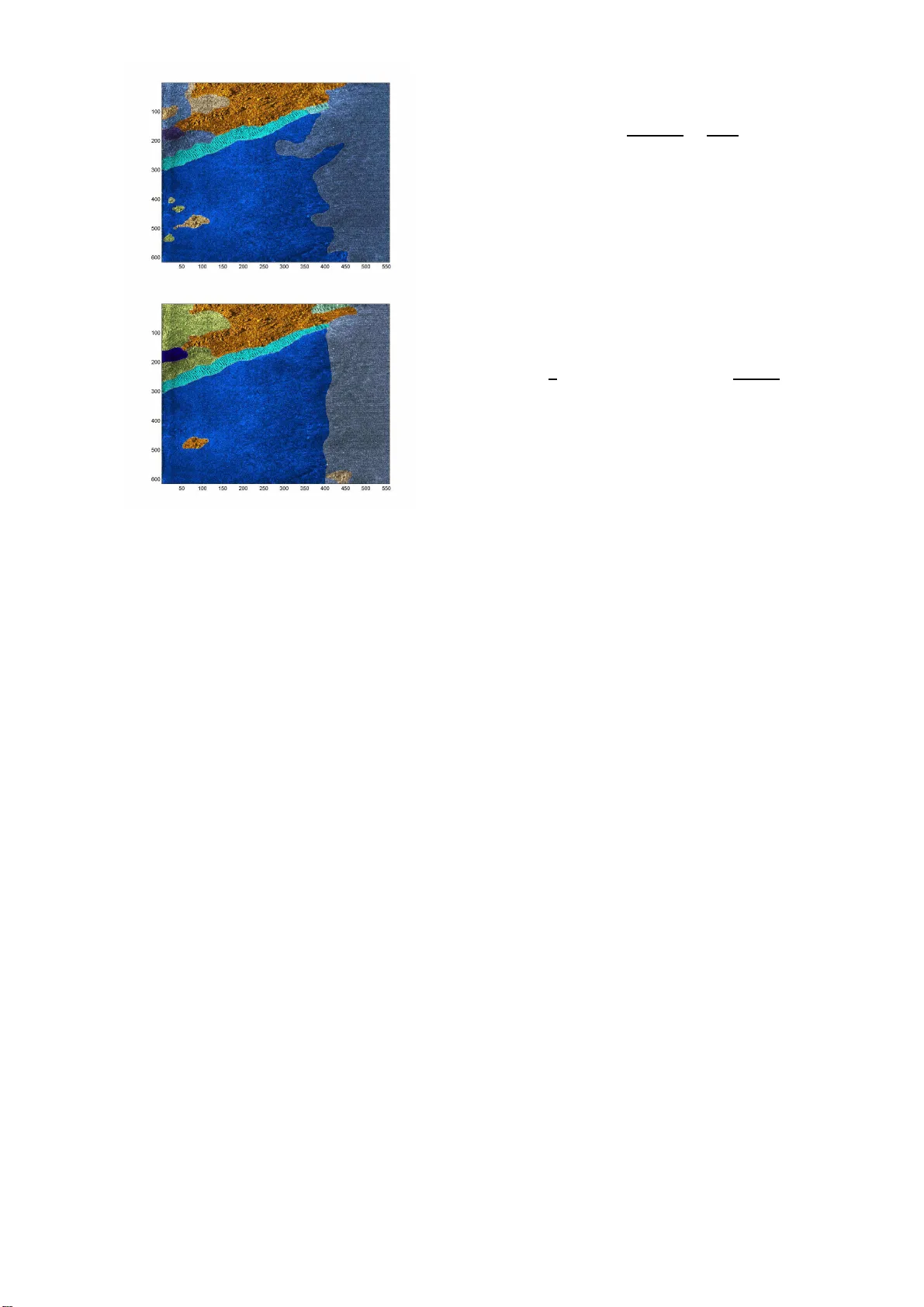
F usion for Ev aluation of Image Class ification in Uncertain En vironmen ts A. Martin E 3 I 2 EA3876 ENSIET A 2 rue F ran¸ cois V ern y , 29806 Brest Cedex 09, F rance Arnaud.Martin@ensieta.fr Abstract - We pr esent in this article a new ev al- uation metho d for classific ation and se gm e ntation of textur e d i mages i n unc ertain envir on ments. In unc ertain envir onm ents, r e al classes and b oundaries ar e known with only a p artial c ertainty gi ven by the exp erts. Most of the time, in many pr esente d p ap ers, only classific ation or only se gmen tation ar e c onsid- er e d and evaluate d. Her e, we pr op ose to take into ac c ount b oth the classific ation and se gmentati on r e- sults ac c or ding to the certainty gi ven by the exp erts. We pr esent the r esults of this m etho d on a f usion of classifiers of sonar images for a se ab e d char acte ri- zation. Keyw ords : I mage classification, I mage segmen tation, Uncertaint y environmen t, Sonar image, F usion of ex p erts, F usion of classifiers. 1 In tro d uction T exture d ima ge cla ssification is a difficult problem in image pro cessing and it is fundamental for a lo t of ap- plications. Many features ca n b e extra cted from the images to cla ssify , a nd ma n y cla ssification algorithms can be use d [1]. Hence, it is rea lly necess ary to ev a l- uate their perfor mance in order to compar e them and choose the most adapted to the application. F or instance, with satellite o r so nar images, hu- man exp erts must b e able to clas sify the types of soils present in the image s . Many types o f s oils ca n b e en- countered in a single image, a nd classificatio n must b e done o n a lo cal part of the image (pixe l- wise, or often on sma ll tiles of e.g. 16 × 16 or 3 2 × 32 pix els) taken as unit for the classificatio n a lgorithm. Hence, after the image classifica tio n, an implicit image s e g ment a- tion is o btained according to the siz e of the tiles. O ne image will b e segmented into several patches, ea c h one corres p onding to a class ( e.g. a sp ecific t y pe of soil). The image class ifica tion methods ar e currently ev a l- uated b y the confusion matrix. Go o d-classificatio n rates and erro r r ates are usually calcula ted from this matrix. W e must know the r eal class of the considered units o f the ima ges in o rder to esta blis h the co nfusion matrix. Confusion matrix does not g ive a n ev aluation of the pro duced segmentation. In or der to ev aluate the segmentation, we can not only consider visual c o mparison b et ween the initial im- age and the seg men ted image. The image seg men ta- tion ev aluation is still a studied problem [2, 3, 4, 5]. W e can consider tw o cas es: we do not have any a priori knowledge of the correct segmentation, o r we hav e an a priori knowledge of the cor rect segmenta- tion. Here we a r e in the seco nd ca se be c ause of the confusion matrix for which we need to get referenced images. In o rder to obtain these referenced images , ex- per ts must manually provide the image segmentation, for example via a visual insp ection. Zhang in [2] g ives a review of usual discrepa ncy measures based on dif- ferent distances b etw een the segmented-pixel and the referenced-pixel. Mos t o f the time, only one mea sure of mis-segmented pixel is given. W e will prop ose on the contrary , in this article a linked study of o ne well- segmented pixel meas ure a nd a mis-seg mented pixel measure. Indeed, in genera l case, if a pixel is not mis- segmented, it is not necessa r y well-segment ed. So we can hav e few mis-segmented pixels but also few well- segmented pixels: the seg mentation is not go o d. W e think that glo ba l image classifica tion ev aluation m ust b e made by ev aluating b oth the cla s sification on considered units (with the confusio n matrix) and in the same time b y the ev aluation of the pr o duced seg- men tation (well-segmented pixe l measure and a mis- segmented pixel mea sure) [6]. In real applica tions, it is really hard for o ne human exp ert to provide a ce rtain information on the c lass and on the b oundaries b etw e e n the c lasses. F or in- stance, the seab ed characterization with sonar imag es cannot b e made b y human exp ert with a sufficient c e r- taint y . These imag es, illustra ting this pap e r, are ob- tained with man y imper fections [7]. Figur e 1 exhibits the differences b etw e e n the interpretation and the cer- taint y of t wo so nar exp erts tr y ing to differentiate the t yp e of sediment (ro ck, cobbles, sand, ripple, silt) or shadow when the infor mation is invisible (ea c h color corres p ond to a k ind o f sediment and the asso cia ted certaint y of the exp ert for this sediment express ed in terms of sure, mo der ately sure a nd not sure). W e prop os e here a new appr oach for textur ed im- age classificatio n and segmentation taking in to account the information g iven by m ultiple e x per ts and their certaint y . In section 2 , we show ho w to integrate the exp ert certaint y in confusion matrix a nd then deduce Figure 1: Segmentation given by tw o exper ts. a go o d-cla s sification r ate and err or classification rate, and how to fuse the different exper t opinions. In sec- tion 3, we prop ose tw o new distance-bas ed mea sures in order to ev aluate well and mis-seg men ted pixel tak ing int o account the ex per ts certainties. This ev aluatio n is illustrated in section 4 on real so nar images, in or der to ev alua te a fusion o f the classifier s pr esented in [7 ]. 2 Image classification ev aluatio n In this section, w e prop os e an o riginal ev aluation a p- proach for cla ssification ba s ed on a new confusion ma- trix taking into a ccount the uncertaint y a nd the pos si- bilit y that o ne unit b elongs more than o ne cla ss. This ev aluation appro ach is a dapted to the image classifi- cation ev aluation, but ca n b e use d for a n y cla ssifier ev aluation. 2.1 Classical Ev aluation A first step of the classica l class ific a tion ev aluatio n ca n be made by comparing the results of the clas sifier to the reality . But in or der to ev aluate a classifica tion alg o- rithm, many different config urations and tests must b e considered. Classification algor ithms c a n y ield ma n y v ariable r e s ults depe nding on the sample. Most of the time, cla ssification algor ithms ev alua tion is co nducted by the confusion matrix. Confusion ma trix is comp osed by the n umber cm ij of elements of the class i class ified in the cla ss j . In order to obtain rates making it easier to compare dif- ferent size of da tabases, we nor malize this confusio n matrix by: N cm ij = cm ij N X j =1 cm ij = cm ij N i , (1) with N the num b er of cons ide r ed classes and N i the nu mber of e le men t fro m the true clas s i . F rom this normalized confusion matr ix a go o d-classificatio n rate vector can b e written as: GC R i = N cm ii , (2) and an err or classification rate vector as: E C R i = 1 2   N X j =1 ,j 6 = i N cm ij + N X i =1 ,i 6 = j N cm ij N − 1   . (3) This erro r cla ssification rate is the mea n of the tw o error s corres p onding to the elements from a given class i classified in another class (firs t term), and corr e- sp onding to the elements c la ssified in a given class j being from another cla ss i (second term). W e do not hav e to normaliz e the first ter m b ecause of the nor - malization o f the confusion matrix on the rows, but the sec ond term must be normalized by the num b er of rows min us one (b ecause o f the N cm ii term co rre- sp onds to the g o o d-classificatio n). Thu s imag e classifica tion algorithms ev a lua tion m ust be made not only on o ne ima g e but on the whole images database. As a co nsequence, we hav e to con- sider a non-norma lized confusion matrix on e a ch imag e and normalize the sum of the matrix confusion on all images of the database. 2.2 Ev aluation with cert ain ty giv en b y eac h exp ert W e consider here a general case wher e information is given by the exp ert on each pixel and the c la ssification algorithm is made on an unit of n × n pixels. Hence on each unit, mor e than one class can b e present. Gen- erally , the classifica tion alg orithms can find o nly one of these c la sses. In o rder to take into account the in- homogeneous units, co nsider tha t if the c la ssification algorithm finds o ne of these classes o n the unit, the algorithm is r ight in the prop or tion of this found cla ss in the n × n pixels-unit and it is wro ng in the prop or- tion of the other classes in the cons idered unit. F or instance, imagine the cas e where the exper t considers a tile of s ize 1 6 × 16 pixels and decla res that on a par t of the unit, 50 given pixels belong to class 1, and 206 other pixels b elong to c la ss 3. If the cla ssification al- gorithm finds the unit b elongs to class 1, the confusio n matrix will be co mputed by the recurr ence relations: cm 11 ← cm 11 + 50 / 2 56 a nd cm 31 ← cm 31 + 206 / 256. Hence the confusio n matrix is not comp osed of in teger nu mbers and N i is also not integer; but the sums of column are still int egers. If the exp ert can give the class with a certaint y grade, we m ust not take equally tw o different grades in o ur cla ssification ev aluation. F or instance, in sonar application, the oper ator ca n b e s ure that o ne part of the image as belong ing to ro ck, and b e totally doubt- ful on another part of the image. Classical confusion matrices supp ose that the r eality is p erfectly known and that is rarely the case esp ecially in image cla ssifi- cation. W e pr op o se to gra dua te this differe nce of info r - mation by differ en t weigh ts cor resp onding to the differ- ent g rades of certa in ty that ar e considered. In the con- fusion matrix, such weigh ts co uld b e integrated eas ily in the ge neral sum. F or example, consider thr e e g rades of certaint y (sure, mo der ately sur e and not sure), we can c ho ose resp ectively the weigh ts: 2/3, 1/2 and 1 /3. If one exp ert lab els a unit as b elonging to the class 1 ( e.g. ro ck), with a mo derate cer ta in ty , and if the classification alg orithm finds the class 1, considering the previo us given weigh ts, the confusion matrix will be up dated suc h as: cm 11 ← cm 11 + 1 / 2. If the classification alg orithm finds the cla ss 2 ( e.g. sand) on the consider ed unit, the co nfusion matrix b ecomes cm 12 ← cm 12 + 1 / 2. Hence the sums of columns are not integer anymore. In order to fuse the referenced images provided b y different exp erts, we can compare the cla ssified imag e with all the r e ferenced images by the exp erts. H ence we obtain as many non-nor malized confusion matrices as exp erts, and we can simply co m bine them by a d- dition. T his can b e done also if the ex per ts do not provide ce rtaint y , in such a case the weight is 1 for all units. By the simple addition of the non-no rmalized con- fusion matr ic e s, we weigh t the obtained results by the image size or the consider ed unit num b er. In order to obtained rates, w e normalize the o b- tained confusion matrix with equation (1) and calcu- late the g o o d-classification r ate vector with equatio n (2) and the er ror classific a tion rate v ector with equa- tion (3). Of cour se these rates are not pe rcentages anymore. F or instance, the go o d- c la ssification r a te is no longer the p erce ntage o f well cla ssified units, b e- cause the weigh ts given by the inho mogeneous units or by the exp ert certaint y are ra tional. These newly obtained co nfusion matrix, g o o d-classificatio n rate and error clas sification rate g ive a go o d ev aluation of clas- sification taking into account the inho mogeneous units and certaint y of the exp erts. This a pproach can b e applied in every domain where we try to classify un- certain elements, and not only in imag e classification. 3 Segmen tation Ev aluation Image classification provides an implicit image segmen- tation, the b oundaries are given by the difference of classes betw een tw o adjacent tiles. A go o d imag e clas- sification ev alua tion ha s to study this o bta ined image segmentation. Many appr o aches ca n be considered in order to ob- tain b oundaries. This is not the sub ject o f this paper and the following segmentation ev aluation ca n be ap- plied to all image segmentations g iven by b oundaries as a succession of pixels . W e prop os e here a linked s tudy of one well- segmented pixel meas ure a nd a mis-seg mented pixel measure. Genera lly one of these measure s is consid- ered in the case with an a priori knowledge [2 , 8, 9]. The well-segmented pixel measure is a well-detection bo undary measure a nd the mis-seg mented pixel mea- sure is a false detection b oundary measure. W e show how these t wo measures can take into account the un- certaint y of the exp ert on the p osition and existence o f the b ounda r ies, assuming that each cer ta in ty g rade is represented by a w eight. 3.1 W ell-d etection b oundary measure First, for each found b oundary pixel f , search the mini- mal distance d f e betw een f and all the b oundary pixels provided by the exp ert e . Hence the pixel e is a func- tion of f , and we should note it a s e f , but in order to simplify notations, it is referred to as e in the rest of the pap er. W e take here an E uclidean dista nc e but a n y other distance can b e envisaged. The certaint y w eight of the pixel e given b y the exp ert is noted as W e . W e define a well-detection criterio n vector by: D C f = exp( − ( d f e .W e ) 2 ) .W e . (4) This criter ion gives a Gaussian-kind distribution of weigh ts with a standard deviation given b y the ce r - taint y weigh ts, a s shown in figure 2. Figure 2: Dista nce weight for the well-detection cr ite- rion. The w e ll- detection bounda ry meas ure is defined by the norma lized well-detection criterio n given by: W DC = P f D C f (max f ( D C f ) . P e W e ) a . (5) Hence, this measur e is defined be t ween 0 and 1. In real applications, this criterion re mains small even for very go o d bounda r y detection, so we can take a = 1 / 6 in order to accentuate small v alues. This criter ion only takes into acco unt t he distanc e from the found b oundar y to the co nt our provided by the exper t. How ever, the r eference b oundar y has a lo cal dir e ction which is another asp ect we hav e to con- sider. Indee d, for instance, a found b oundary can cross a given bounda ry orthog onally: in this case some pix- els from the found b oundar y are very near (in terms of dista nce) to pixels from the reference bo undary but that is not a go o d detection. In o r der to take into a ccount the lo ca l direction, we count, for a g iven pix e l f of the found boundar y , how many pixels from the found b oundary are linked by the minimal distance to the same pixel e of the refere nce bo undary . This num b er is noted n ef , e.g. on fig ure 3 we hav e n ef = 3 fo r three different f . W e redefine the well-detection bo undary measure by: W DC = P f D C f /n ef (max f ( D C f /n ef ) . P e W e ) a . (6) Figure 3: Example o f n ef for three given f , the found bo undary is repres en ted by g reen squar es a nd the ref- erenced b oundary b y a black line. The pro blem is that the num b er n ef do es not ad- equately r epresent a n umber of pixels on the sa me bo undary and ta ke into a ccount only o rthogonal di- rection. Howev er this measur e gives a g o o d ev aluation of the prop ortion of the found b oundaries. 3.2 F alse detection b oundary measure The false detec tio n b oundary mea sure is base d on the same pr inc iple as the well-detected b oundary measur e, but the Gauss ian-kind distribution of weigh ts m ust b e inv ersed. Hence we can defined a false detection cr ite- rion by: F DC f = 1 − D C f /W e , (7) where the pixels f and e a re linked by the minimal distance d f e . As a consequence, the false detection bo undary measure ca n b e defined by the normalized false detectio n criterion by: F D = 1 − exp  − P f ( F D C f .n ef ) max f ( F D C f .n ef ) . P e W e  . (8) Here we hav e describ ed the tw o measures F D and W DC that c o mpare tw o images: o ne image cla s sified by the algorithm and the other one provided b y only one ex per t. In order to ev aluate image seg mentation al- gorithms on many images and/or fuse the exp er t opin- ions, we can use a weigh ted sum o f these b oth mea- sures. The weights are given by the image sizes, whic h can b e differen t for all considered images. 4 F usion of classifiers of sonar images W e prese n t here our imag e classification and segmenta- tion ev aluation in a fusion of cla ssifiers of so nar images presented in [7 ]. Indeed, underwater environmen t is a very uncertain environmen t and it is particularly im- po rtant to classify seab e d for numerous a pplications such as Autonomous Underwater V ehicle navigation. In recent sonar works ( e.g. [10, 11]), the cla ssification ev aluation is made only by vis ual compariso n of o ne original image and the cla ssified image. Tha t is not satisfying in order to co rrectly ev alua te image classifi- cation and seg men tation. 4.1 Database Our databas e con ta ins 42 sonar imag es provided by the GESMA (Groupe d’Etudes Sous-Marines de l’A tlantique). These imag es were obtained with a Klein 5400 lateral sonar with a reso lutio n o f 20 to 30 cm in azimuth and 3 cm in range . The s ea-b ottom depth was betw een 15 m and 40 m. Three ex per ts hav e manually seg men ted these im- ages giving the kind o f s e dimen t (ro ck, co bble, s and, silt, ripple (horizontal, v ertica l or at 45 degr e es)), shadow or other (typically ships) parts on ima ges, helpe d by the manual s egmentation interface presented in fig ure 4. All s edimen ts are given with a certa int y level (sure, modera tely sure o r not sure), and the bo undary b etw een tw o se diments is also giv en with a certaint y (sur e, mo derately sure or not sure). Hence, every pixel o f every imag e is lab eled as being either a certain type of se diment or a shadow or other, or a bo undary w ith one of the three certa in ty lev els. W e choose the weigh ts: 2/3, 1 /2 and 1/3, for res pectively the certaint y le vels: sur e, moder ately s ure a nd not sure. The prop or tion of ea ch sediment given by the three expe r ts are g iven in the table 1. Note that the prop ortion of the differen t s edimen t are very different and that ca n be a problem for the classificatio n. The prop ortions are very similar for the three exp erts. W e see that sand and silt ar e the mos t pres e n t a nd the shadow and other ar e very few r epresented on thes e images. Figure 4: Manual Segmentation Interface. 4.2 F usion approac hes W e consider here four methods of features extrac- tion based on four r epresentations of the image: T able 1: Pr op ortion of sediment in the da tabase (%) Exp ert 1 Expert 2 Exp ert 3 Ro ck 9.64 9.6 2 12.78 Cobble 6.00 3.7 1 8.4 2 Ripple 13.96 15.98 13.53 Sand 26.97 35.62 28 .4 0 Silt 42.85 34.57 35 .2 0 Shadow 0.55 0.4 4 0.2 6 Other 0.10 0.0 5 1.4 0 co-o ccurr ence matrices, run-le ngths matrix, wav elet transform and Gab or filters [7]. They pr ovide resp ec- tively 24, 20, 6 3 and 4 para meter s. These four feature sets are indep endently co ns idered as the inputs of a m ultilay er p er c eptron (MLP) classifier presented in [7]. In order to illustrate our ev aluation approach o nly tw o of the classifiers fusion presented in [7] are co nsidered coming from the evidence theor y . The evidence theory is based o n bas ic b elief assig n- men ts (bba) defined by mapping of each subset o f the space of discernment Θ = { C 1 , , C n } onto [0 , 1], such that: X X ∈ 2 Θ m ( X ) = 1 , (9) where m ( . ) represents the bba. The principal difficulty is the choice of a bba ac- cording to the application. W e can co nsider tw o types of a pproaches: one ba sed o n a probabilistic mo de l [12] and ano ther one bas ed on distance transfo r mation [13]. Appriou in [1 2] pro po ses tw o equiv alent mo dels bas e d on three axioms. The first one that we use in this arti- cle in or der to fuse the decisions of the four classifier s is given by:              m j i ( { C i } )( x ) = α ij R j p ( q j | C i ) 1+ R j p ( q j | C i ) m j i ( { C i } c )( x ) = α ij 1+ R j p ( q j | C i ) m j i (Θ)( x ) = 1 − α ij (10) where q j is the j t h classifier (supp osed c o gnitively independent), j = 1 , ..., m , α ij are reliability co effi- cients on each clas sifier j for each class i = 1 , ..., n (in our application w e take α ij = 1), and R j =  max q j ,i p ( q j | C i )  − 1 . The approach prop osed in [13] is used in order to fuse the numerical outputs of the four class ifiers. The bba ar e g iven by:    m j i ( { C i } /x ( t ) )( x ) = α ij ϕ i ( d ( t ) ) m j i (Θ /x ( t ) )( x ) = 1 − α ij ϕ i ( d ( t ) ) (11) where  x ( t )  is a set of learning v ec to rs, d ( t ) = d ( x, x ( t ) ) is a distance b etw e e n x and x ( t ) and C i is the class o f x ( t ) . ϕ i is a distance function given b y: ϕ i ( d ) = exp( − ν i d 2 ) , (12) where ν i is a p ositive pa r ameter asso c ia ted to the cla ss C i . The co m bination of the bba is ba s ed on the o r thog- onal non-norma liz ed Dempster- Shafer’s rule given in [14] for all X ∈ 2 Θ by: m ( X ) = X Y 1 ∩ ... ∩ Y M = X M Y j =1 m j ( Y j ) , (13) where Y j ∈ 2 Θ is the resp onse of the ex per t j , and m j ( Y j ) the asso cia ted b elief function. In order to co n- duct the dec ision, we consider the maximum of pignis- tic probability [1 5]. 4.3 Ev aluation Here, we consider six different cla sses given by the table 2. The images are consider ed as a succes sion of tiles of size 32 × 32 pixels. Hence the 42 images provide 38 997 tiles, units for the clas sification. The pr o po rtion of the nu mber o f different sediments o n a tile is given in the table 3 for ea ch exp e rt. These prop or tions are very similar for the three exp erts. T able 2: Repar tition of the kind of sediment in cla sses class sediment class 1 rock class 2 cobble class 3 ripple class 4 sand class 5 silt class 6 shadow a nd other T able 3: Prop ortio n of num b er of different kind of sed- imen ts on the tiles (%) Exp ert 1 Expert 2 Exp ert 3 1 sediment 77.79 79.65 79 .9 4 2 sediments 20.70 19.30 19 .3 3 3 sediments 1.48 1 .0 3 0.7 2 4 sediments 0.04 0 0 5 sediments 0 0 0 6 sediments 0 0 0 The total conflict betw een the three exp erts is 0.2244 . This conflict comes ess ent ially from the dif- ference o f opinion of the ex per ts a nd not from the tiles with more than one sediment. Indeed, w e hav e a weak auto-c onflict (conflict coming from the combination o f the same exp ert three times). The v alues of the auto- conflict for the three exp erts are: 0 .0 496, 0.04 74, and 0.0414 . The databa se is divided into three parts. The first part comp osed of 20 images (with only 125 05 tiles) is used for the lear ning step of the multila yer p erceptron. A second part of 10 ima g es (compo sed of 12650 tiles) serves the learning step of b oth the fusion appr oaches. The used information for these learning stages are only considered given by one of the three exp erts (exp er t 1). The last 12 images (corr e spo nding to 138 41 tiles) ar e used in order to ev aluate the classifier fusion metho ds, considering the info r mation given by the tw o other ex- per ts. The figur e 5 describ es the manual segmentation made by one exp ert and the a uto matic classifica tion reached by b oth class ifier fusion metho ds. The dark blue par t corresp onds to the no n considered part o f image. First at all if w e lo o k o n figure 5 the r esults of the classifica tion of the sa me image, we note that the sediments ar e quite well classified. Ho wev er, just lo oking this figure 5 we can not say if the clas sification is go o d or not, and if one fusion appr oach is b etter or not: it remains very s ub jectiv e. Moreover it could be go o d for this image and not for other s . So we prop os e to use o ur measures . Figure 5: Man ua l seg mentation (firs t) and automatic segmentation given by the pro babilistic appr oach (sec - ond) and the distance a ppr oach (third). First w e compar e the obtained results to the infor- mations given by only the exp ert 2. The obtained nor - malized confusio n matrix on the test data ba se is given by for the probabilistic appr oach:                    ro ck cobble ripple sand silt other 0 . 00 0 . 01 0 . 00 0 . 01 0 . 01 99 . 97 13 . 49 2 4 . 62 0 . 00 33 . 31 0 . 00 28 . 57 5 . 37 2 . 92 47 . 70 22 . 33 3 . 46 1 8 . 22 8 . 78 3 . 10 6 . 97 59 . 51 21 . 05 0 . 59 0 . 20 0 . 28 0 . 99 16 . 41 82 . 10 0 . 00 39 . 45 0 0 0 29 . 57 30 . 97                    and for the distance approa ch by:                    ro ck cobble r ipple sand silt other 0 0 . 01 99 . 97 0 . 01 0 . 02 0 0 32 . 05 20 . 7 4 34 . 05 1 3 . 16 0 0 2 . 90 51 . 51 9 . 28 36 . 31 0 0 2 . 24 4 . 08 28 . 93 6 4 . 74 0 0 0 . 00 0 . 14 4 . 42 95 . 44 0 0 0 30 . 96 0 6 9 . 03 0                    W e note that the dis ta nce appro ach do es not clas- sify r o ck and other. The mos t of tiles are classified in ripple and silt a nd few in sand. The probabilistic approach provides a full confusion ma trix. In order to summar ize these results, we can give the vector of go o d-classifica tion ra te and the vector of erro r clas s ifi- cation r ate g iven b y [0 2 4.62 4 7 .70 59 .51 82.1 0 30.9 7 ] and [94 .30 59.1 3 54.55 82.84 7 1.18 14 8.05] for the pr ob- abilistic approach and by [0 32 .05 51 .51 28 .94 9 5 .44 0 ] and [50.00 6 4.03 144.84 72 .88 1 49.43 50 .00] for the dis- tance approach. W e r e c all that is not a per centage be - cause of the weight s. The vector of go o d- c lassification rates c a n pr ovide a mean of go o d-class ifica tion rate. W e obtain here 62.43 for the pro babilistic a pproach and 50.5 5 for the distance a ppr oach. These results tend to prov e that the pr obabilistic appro a ch gives b et- ter results tha n the distance approach. W e ca n a lso study the differ e nce o n ho mo geneous tiles and inhomo- geneous tiles. F or instance , for the proba bilistic-based approach, the normalized confusion matrix on homo- geneous tiles is given by:                    ro ck cobble ripple sand silt other 0 0 0 0 0 1 00 . 00 13 . 49 2 4 . 62 0 3 3 . 31 0 28 . 58 5 . 37 2 . 92 47 . 70 22 . 33 3 . 46 18 . 2 2 8 . 78 3 . 10 6 . 97 59 . 51 21 . 05 0 . 59 0 . 21 0 . 28 0 . 99 16 . 41 82 . 10 0 0 0 0 0 0 0                    and on inhomog eneous tiles:                    ro ck cobble ripple sand silt other 25 . 50 1 1 . 12 7 . 41 15 . 09 14 . 14 26 . 7 3 20 . 97 1 7 . 84 8 . 32 34 . 02 8 . 15 10 . 71 13 . 50 5 . 71 30 . 29 29 . 73 7 . 7 5 13 . 02 11 . 21 5 . 79 11 . 86 44 . 95 21 . 33 4 . 8 5 13 . 79 3 . 24 10 . 24 16 . 40 53 . 55 2 . 7 7 39 . 46 0 0 0 29 . 58 30 . 97                    W e observ e an imp or ta n t difference. The go o d- classification rate is b etter on the ho mogeneous tiles (62.43) tha n on the inhomogeneo us tiles (39.99). Hence the c la ssification of the inhomog e neous tiles is a rea l difficult y . The figure 5 seems to show that the segmentation of the distance approach is better than the probabilistic approach. W e hav e to ev a luate the seg men tation pr o- ducted by the clas sification with our measures. Note that this ev aluation is hig hly dep ending on the size of the tile, here: 32 × 32 pixels. Our prop os ed mea- sures, given resp ectively by the equations (6) a nd (8) expressed in p ercentage, pr ovide in the case of prob- abilistic approa ch 59.84 for the well-detection crite- rion and 45.64 for the false ala rm criterio n, a nd for the dis tance approa ch 5 7.22 for the well-detection cr i- terion and 48.5 4 fo r the false ala rm criterio n. The well-detection criterion a nd the false alarm c r iterion of the proba bilis tic-based fusion a r e b etter than the well-detection criterion of the dista nce-based fusion. How ever, we hav e to take care of both measures that are studying together. Indeed, on the figure 5, the probabilistic-ba sed metho d provides a lo t o f bo und- aries, and so the c ha nce to contain w ell-detection cr i- terion incr eases, but the false alarm incr eases also. In order to confir m these r esults, we can fuse easily these measures with the resulted measures obtained with the exp ert 3. The g o o d- classification ra te and error clas sification rate vectors a re resp ectively given by [26.73 14.54 39 .83 60.56 81 .8 3 0] and [6 1 .71 57.01 58.47 1 09.05 111.8 9 7 4 .16] for the probabilis tic- based metho d and [0 1 7.94 48.02 30.0 9 95.83 0] and [50.00 63.31 70.10 87.40 169 .5 4 5 0 .00] for the distance-based metho d. The mean of the go o d-class ifica tion ra te is 58.39 for the probabilistic- based metho d and 49.2 4 for the distance- based metho d. The results of the seg - men tation ev aluation are given by the well-detection criterion a nd the false alarm criterion: resp ectively 62.76 and 54.57 for the pr obabilistic-based approach and 60.83 and 55.90 for the distance-based appro ach. The fusion of measures o riginally from the exp erts shows that the pr obabilistic-based metho d is b etter than the distance- based method. How ever the differ- ence is lower than w ith only one exper t. 5 Conclusions W e ha ve prop osed a new ev aluation o f the image clas- sification and segmentation based on new meas ures in uncertain environments. In o rder to achieve a g o o d ev aluation of the image classification, we hav e seen that a linked study of the class ification and of the pro duced segmentation is necess ary . The prop os ed clas sification ev aluation can b e used indepe ndently for every kind of uncerta in units classifica tion, e.g. is a basic b elief assignment is asso ciated to the units. The pro po sed segmentation ev aluatio n can b e us e d for a ll image seg- men tation approa ches and not only for a segmentation pro duced by a classifier . The pr op osed co nfusion ma- trix takes into a ccount the uncertaint y of the exp ert and als o the inhomogeneo us units ( e.g. patch-w o rked images in the case of imag e classification). Moreover we have defined g o o d-classificatio n and errors c lassifi- cation rates from o ur confusion matr ix. The prop os e d segmentation ev alua tion conside r s go o d and false de- tection b oundary mea sures where the sub jectivit y of the exp ert is considered by the given uncertaint y . In our prop o sed ev aluation a pproach, the fusion of exp erts opinio ns is made by the fusion o f our differ- ent mea sures calculated for ea ch ex per t. This fusion is made b y using a simple sum: the uncerta in t y is con- sidered directly in our measures. It can be interesting to fuse the informatio ns provided by exper ts b efore the ev aluation in order to obtain an uncertain and impre- cise r eality . This new reality c a n used for instance for learning and also for the ev alua tion of cla s sifiers. References [1] J.C. Russ, The Image Pr o c essing Handb o ok , CR C Press, 200 2. [2] Y.J. Zhang , A s ur vey on ev aluation methods for images segmen tation, Patt ern R e c o gnition , V o l. 29, No. 8 (1996), 133 5-134 6 . [3] Y.J. Zhang, Ev aluation and compar ison of differ - ent se gment ation algo rithms, Patt ern R e c o gnition L etters , V ol. 18, Issue 10 (1997 ), 96 3 -974. [4] R. Rom´ an-Rold´ an, J.F. G´ omez-Lo p er a , C. A tae - allah, J. Mart ´ ınez-Aroza and P .L. Luque- Escamilla, A measure of qualit y for ev alua ting metho ds o f seg men tation and edge detection, Pat- tern R e c o gnition , V ol. 34, Is sue 5 (2 001), 969 - 980. [5] J.B. Mena a nd J.A. Malpica, Color imag e segmen- tation based o n three levels of texture statistical ev aluation, Applie d Mathematics and Computa- tion , V ol. 161 (2005 ), 1- 17. [6] A. Mar tin, H. La anay a, and A. Arnold-B os, Ev al- uation for Uncertaint y Imag e Classificatio n and Segmentation, ac c epte d in Pattern R e c o gnition Journal . [7] A. Martin, Compar ative study of information fu- sion metho ds for sona r imag es classification, The Eighth International Confer enc e on Information F usion, Philadelphi a, USA , 25-29 July 20 0 5. [8] T. K anoungo, M.Y. Jaisimha, J. Palmer and R.M. Haralick, A Metho dolog y for Quantitativ e Perfor- mance Ev aluation of Detection Algorithms, IEEE T ra nsactions on Image Pr o c essing , V ol. 4, No 21 (1995), 1 6 67-16 73. [9] T. Peli and D. Malah, A Study of Edge Detec- tion Alg orithms, Computer Gr aphics and Image Pr o c essing , V ol. 2 0 (1982), 1-2 1. [10] G. Le Chenadec, and J.M. Boucher, Sonar Im- age Segmen tation using the Angula r Dep endence of Ba ckscattering Distributions, IEEE Oc e ans’05 Eur op e, Br est, F r anc e , 20 - 23 June 2005 . [11] M. Lianantonakis, and Y.R. Pet illot, Sidescan sonar s egmentation using active con tours and level set metho ds, IEEE Oc e ans’05 Eur op e, Br est, F r anc e , 20-2 3 June 2005. [12] A. Appriou, Situation Assessment Based on Spa- tially Ambiguous Multisensor Measurements, In- ternational Journ al of Int el ligent Syst ems , V ol 16 , No 10 , pp. 1135-1 166, 200 1. [13] T. Deno eux, A k-neares t neighbor classifica tion rule based on Dempster-Shafer Theory , IEEE T ra nsactions on S ystems, Man and Cyb ernetics , V ol 25, No 5, pp. 804-9 13, 19 95. [14] Ph. Smets, The Combination o f Evidence in the T ra nsferable Belief Mo del, IEEE T r ansactions on Pattern Analysis and Machine Int el ligenc e , V o l 12(5), pp 447-458 , 1 990. [15] Ph. Smets, Constructing the pignistic pro bability function in a context of uncertaint y , Unc ertainty in Artificia l Intel ligenc e , V ol 5, pp 29 -39, 1 990.