Alternative formulas for synthetic dual system estimation in the 2000 census

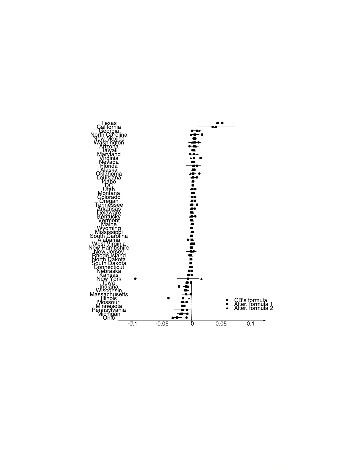
IMS Collectio ns Probability and St atistics: Essays i n Honor o f David A. F reedman V ol. 2 (2008) 90–113 c  Institute of Mathematical Statistics , 2008 DOI: 10.1214/ 19394030 70000004 00 Alternativ e form ul as for syn thetic dual system e stimation in the 2000 cens us La wrence Bro wn ∗ 1 and Zhan yun Zhao † 2 University of Pennsylvania and Mathematic a Policy R ese ar ch Abstract: The U.S. Census Bureau provides an estimate of the true p opula- tion as a supplemen t to the basic census n um bers. This estimate is constructe d from data i n a post-censal survey . The ov erall pro cedure is referred to as dual system estimation. D ual system estimation is designed to pr oduce revised es- timates at all l ev els of geograph y , via a synthet ic estimation pro cedure. W e de sign three alternat ive form ulas for dual system e stimation and in- v estigate the differences in area estimates pr oduced as a result of using those formulas. The pr imary t arget of this exercise is to better understand t he nature of the homogeneit y assumptions in v olve d in dual system estimation and their consequenc es w hen used for the en umeration data that occurs in an actual large scale application like the Census. (Assumptions of this nature are some- times co llectiv ely referred to as th e “syn the tic assumption” for dual system estimation.) The sp ecific fo cus of our study i s the tr eatment of the category of census coun ts referr ed to as imputations in dual system estimation. Our results show the degree to which v arying treatmen t of these imputation coun ts can result in differences in p opulation estimates for local areas such as states or counties. 1. In troductio n The U.S. census is required b y the Constitution to be conducted every ten years. In an attempt to provide b etter estimates of the true population than con tained in the basic cens us c o unt s, the Census Burea u [ 13 ] use s b o th statistica l a nd demo - graphic metho ds. In 2 000 the statistical pro ce ss w as called Accuracy and Cov erage Ev alua tion (A.C.E.). The 200 0 A.C.E. da ta c o nsists of tw o par ts: the Population sample (P-sample) and the Enumeration sample (E- sample). The P -sample includes p erso ns who ar e v alidly included in the A.C.E. survey , and the E-sample includes census enumera- tions from househo lds in the A.C.E. blo ck cluster s. F or a detailed ov erview o f the 2000 A.C.E., plea s e s ee Hogan [ 9 ] and Norwo o d and Citro [ 11 ]. The 2000 A.C.E. was designed to get a n es timate of the p opulation at every geogr a phic level, based on the census count and the informatio n from the E-sample and the P-sa mple. T o b e more precise, the pro cedure adopted b y the Census Bur eau is ter med a synthetic dual system estimate. Its v alidit y res ts on several assumptions, including a ma jor synthetic (homogeneity) assumption. ∗ Supported in part b y NSF Grant DMS-99-71751. † Supported in part b y National Researc h Council of the National Academy of Sciences. 1 Unive rsity of Pennsylv ania, 400 Jon M . Huntsman Hall, 3730 W aln ut Street, Philadelphia, P A 19104, USA, e-mail : lbrown@w harton.u penn.edu 2 Mathematica P oli cy Rese arc h, Inc ., P .O. Box 2 393, Princeton, NJ 08543, USA, e-mail : zzhao@ma thematic a-mpr.com AMS 2000 subje ct classific ation. 62D05. Keywor ds and phr ases: dual system estimation, imputation, syn the tic a ssumption, undercount . 90 Alternative f ormulas in the 2000 c ensus 91 V arious tec hnical assumptions can be made for synthetic assumption. These affect the details o f the formulas needed to pro duce the final p opulatio n estimates. F or ideal and homo g eneous p o pulations any of the resulting for mulas will pro duce un biased estimates. How ever, the U.S. populatio n do es no t app ear to hav e this type of idea l structure. Hence different synthetic a ssumptions yield different estimates, and it do es not app ear that all of these estimates are a ctually unbiased. This pap er inv estigates the na tur e of these as sumptions a nd the exten t o f the differences pro duced w hen using three alternative dual sy s tem formulas within the 2000 U.S. Census. It should b e emphasized tha t the da ta av ailable to us do not allow us to mak e a ny co nfident claim as to which o f the estimates is more accurate; indeed s uch a claim is not o ur ob jective. Instead, we pr esent our analyses a s a means of pr oviding better under standing of the dual sys tem estimatio n pro cess in the prese nce o f actual p o pulations, such as that enco unt ered in the 2000 Census, and of judging the extent of differences that may be exp ected to result from differing assumptions ab out the census enumeration pro cess. Our analysis r evolv es around the exten t and homog eneity of imputations o f household and whole p ers on r e cords into the census enumeration. The av ailable data allows us to pro duce alternative estima tes ba sed on different treatment o f these imputatio ns . As we later r emark, there are other asp ects of the dual sys tem pro cess that might inv olve a nalogous biases in the presence of inhomogeneity , how- ever the data av ailable to us do not allow fo r as c o mplete an analysis rela tive to those factor s. In Section 2 we briefly discuss the natur e a nd extent of imputatio n in the 20 00 census. It is c le a r that the desired sto chastic homogeneity do es no t ho ld there. Section 3 introduces background for dual sys tem estimation and the sy nt hetic as- sumption. The alternative formulas a re presented in Sec tio n 4. Section 5 displays the results of using these formu las to estimate the tr ue p opulation shares of the states in 2000 . Section 6 presents similar results for estimation o f p opula tion shares of gr oups of counties. Mathematical compariso n of differen t formulas is made in Section 7. Section 8 contains a summar y conclusio n a nd remark s. The da ta for A.C.E. was collected during the 200 0 census and first pr epared and analyzed b efore April 20 01. The Census Burea u decided not to issue the r esults then pro duced as o fficial census estimates. F o llowing this, the data was re-a nalyzed several times, le a ding up to revis ed A.C.E. estimates, re ferred to as A.C.E. Revi- sion I I. These were released on March 2003. The revised data iden tified, a nd deleted from the estimation pro cess, a significant num ber of r ecords tha t were judged to be duplicates . Ther e were als o a num b er of other more technical, but not insig nif- icant, innov ations in A.C.E. Rev is ion II. See Kostanich [ 10 ] for a mor e co mplete description of A.C.E. Revis io n I I. The analyses o f o ur pa per are bas ed on the original Apr il 2 001 A.C.E . da ta. There are several reaso ns for our using this o r iginal data, r ather than the revised A.C.E. I I data. The primar y reaso n is that this is the data that was supplied to us by the Bure au, b eginning in 2 001. (W e g ratefully a ckno wledge the Bureau’s assistance in s upplying us with suita ble versions of this data.) F urthermo re, our purp ose has b een to understand the natur e of traditional dual system estimation, and the conse q uences of alterna te synthetic assumptions. F or the mo st par t the nature of the Apr il 2 0 01 A.C.E. data in relation to the census is a nalogous to that betw een earlier censuses and their dual system surveys. (In particular, bo th the 2000 census counts and the 2001 A.C.E. da ta contain c orresp o nding ly s ig nificant num bers of duplica tes, such a s presuma bly e x isted in earlier cens us data even though there was no way to explicitly identify them. See Sectio n 2 o n imputation for discussion 92 L. Br own and Z . Z hao of one difference be tw een 2000 a nd earlier census es.) F urther more the a nalysis of A.C.E.I I in volv es a n um ber of sp ecial complicatio ns and assumptions b eyond thos e of the standa rd dual system analyses . 2. Imputation W e use I I , the Census Burea u’s notation, to denote the num ber of imputations . T echnically I I is referr ed to as “insufficie nt information” . It is not unusual for some census records to contain inco mplete informa tion to a mo dest e xtent . If all or nearly all rele v an t information is missing so that the matching of the P-sa mple records to the E-sample enumerations is not feasible, then the r e cord is describ ed as having insufficient infor mation. Here we use the word “imputatio n” gener a lly to describ e records that for so me reaso n do not include eno ugh information to b e included in the A.C.E. pro cess. Broa dly s pe a king, census imputatio n also includes imputation for item no n-resp onse for r ecords in the A.C.E., and imputation for matching status in the A.C.E. pro ces s. Y et in our con text, imputatio n is r eferred to as the whole records not included in the A.C.E. pro c e ss due to ins ufficient information. In the 2000 census, imputations included tw o parts: inhere nt imputation and late adds. One can identify t w o basic kinds of inherent imputation. Sometimes w e do know with reas onable certaint y how ma n y people there are in the household, but la ck per sonal infor mation ab o ut them as is needed for the matching o f the E-sa mple and the P-sample in the dual sys tem pro cess. In this ca se, we just need to impute demographic infor mation for each p erso n. On the other hand, sometimes the actual nu m ber of p eople in the ho usehold is als o unknown. In this circumstance b oth the true counts and p erso nal infor mation need to be imputed. It is even p ossible to give a finer sub divisio n of types of inherent imputations. See Norwo o d and Citro [ 11 ]. Imputation re lated to a large num ber o f late-a dds was a sp ecial fea ture of the 2000 census. B e cause of its concer n a b o ut address duplica tion, the Census Bur eau created a sp ecial re s earch prog ram just after the ba s ic cens us data was c ollected. The Bur e au was able to iden tify , and pulled out, approximately 6 millio n p ers o n records in 2.4 million hous ing units a s p otential duplicates . La ter on, a ppr oximately 2.4 million per sons in 1 million housing units were reinstated in to the census. How- ever, this was to o late for the 2.4 million p eople to b e included in the A.C.E. pro cess. Hence they were referred to as “Late Adds” and were treated similar ly to imputation da ta. F or details of resea rch on duplica tes, see ESCAP [ 4 ]. T able 1 is a compariso n of the dis tributions of imputation in 1990 a nd 200 0. Besides the fact that there was no sp ecia l tre a tment for La te Adds in the 199 0 census, there is a sig nificant difference in terms of the r a tio o f imputations from households with known perso n coun t and imputations from households with un- known per son co un t b etw een the 19 90 and the 2000 Census. In 20 00, that r atio was ab out 4. Y et in 1990 , the ratio was 44 which is 1 0 times la rger than tha t in 200 0. T a ble 1 Numb er of imputations ( I I ) as a p e r centage of c e nsus c ount ( C ) Imputation type 2000 Census 1990 Census Kno wn Person Count 1.68 0.88 Unkno wn P erson Count 0.43 0.02 Late Adds 0.85 0.00 T otal 2.96 0.90 (Source: The 2000 Census: Interim Assessment ) Alternative f ormulas in the 2000 c ensus 93 The p ercentages of I I fr o m the 198 0 census were mor e s imila r to thos e of 2000 than were the 19 9 0 p erc e n tages. In this pa pe r , the item C − I I denotes the num b er of p eople with full informa tio n. They a re frequently refer red to as “ data-defined” p er sons, and we use D D to denote the num b er of them in the fo llowing sections. 3. Dual system estim ation As w e int ro duced befor e, the 2000 A.C.E. data consists of the E -sample and the P- sample. Based on the information of the E-sample a nd the P-sample, a dual sy stem estimate of the p opulatio n is pro duced for sp ecia l subgr oups, ca lled p ost-s trata. These p os t- strata estimates are then app or tio ned and r e combined so as to for m estimates for any geo graphic ar ea, such as state, count y , census blo ck etc. W e now discuss some asp ects of this pro cedure . 3.1. Post-str atific ation F or the purp ose of analysis, the popula tion is divided in to c e rtain groups called post- strata. Sixty-four p ost-stra tum gro ups were crea ted based on informa tio n ab out geogr a phic lo ca tion, race, Hispanic origin, ho us ing tenure etc. In addition there were 7 age/s ex ca teg ories. Thus originally there were 448 p ost-stra ta. La ter on, some small po st-strata were collaps e d together to form 416 final po st-strata. [See T able 5 in the App endix for details of the constr uction of p o s t-strata.] 3.2. Dual system estimati on The dual system es timate fo r po st-stratum i can b e written as (1) d D S E i = D D i × d C R i × 1 d M R i . Here D D i is the num ber of data -defined p erso ns in p ost-s tratum i . d C R i and d M R i are the estimates of the E-s a mple correct en umeration rate and the P-sample matching rate resp ectively . In the E -sample, enumerations are divided into tw o catego ries: corr ect enumer- ations and erro neous enumerations. T he co rrect enu meration rate meas ures the accuracy of the c e nsus. It is estimated as (2) d C R i = C E i C E i + E E i , where C E i denotes the num b er of corr ect enumerations and E E i denotes the n um- ber of err o neous enumerations in p ost-stra tum i . The P -sample per sons are taken int o a matching pro cedure to see whether they can b e matched with p er sons in the E-sa mple. The P-sample matching rate then measures the cov erage of the cens us . The formula for d M R i is more complicated than that for the other e lement s o f ( 1 ), and it is not par ticularly p ertinent to the current consider ations. The reader should consult Hoga n [ 8 ] for details. Since it w as adopted b y the Cens us Bureau to estimate the populatio n, the dual system estimation metho d has be e n considered in principle a la rge-sc a le capture- recapture pro c e dur e. It can b e motiv a ted from a n ov er-simplified, primitive mo del 94 L. Br own and Z . Z hao for capture-rec a pture estimation. In this mo del, the interrelation o f the P- sample and the E-s a mple can b e schematically s ummarized in a tw o by tw o table, and elements in the t wo by tw o table ar e estimated ba sed on the assumption of the independenc e of the E-sa mple a nd the P-s ample. F o r a deta iled overview of dual system estimation, see Hog an [ 7 ]. 3.3. Synthetic assumption The census provides po pulation figures for geographic s ubdivis ions m uc h smaller than those defined b y p o s t-stratum b oundaries . These “smaller ar eas” include states, congress ional districts, metrop olita n areas, and even divisions a s small as census tra c ts and ce ns us blo cks within tracts. In order to g et smaller ar e a es timates, the estimates d D S E i for each p os t-stratum m ust be divided up and appor tioned to geo g raphic a r eas lying within that post- stratum. This pro cedure is called synthetic estimatio n a nd the assumption(s) that suppo rt its v alidit y is (ar e) referr ed to a s the sy nt hetic assumption. It seems to us that ther e are v ar ious reas o nable for ms of synthetic as sumptions that co uld b e prop ose d, and these lead in practice to differe n t smalle r area po pu- lation estimates . F or now we first pres ent the for m ula implement ed by the Bureau. Then we later contrast it w ith alter native formulas that also seem to us to b e plausible. F or the purp ose of synthetic estimation, the Ce ns us Bureau a ssumes that the estimate, d D S E i , s ho uld b e divided in pr op ortion to the tota l cens us c o unts within its p ost-s tratum. Let the index k , k = 1 , 2 , . . . , K i refer to g eogra phic subr egions within pos t-stratum i . Let C ik denote the total cens us counts for p os t-stratum i and region k , and let C i denote the totals for the po st-stratum. The Bureau po pulation estimate for p os t-stratum i r egion k is then called d D S E ik or S ik and is given by the formula (3) S ik ≡ d D S E ik = C ik C i d D S E i . This reflects the Bureau’s synthetic assumption that the p opula tio n dis tribution for smaller ar eas within a p ost-s tr atum is ho mogeneous with resp ect to the census counts for those a reas within that p ost-s tr atum. F or mula ( 3 ) is often rephra s ed in a differe n t but equiv alen t format. Define the Cov erage Corr ection F actor for p ost-s tr atum i ( C C F i ) by (4) C C F i = d D S E i C i . Then (5) S ik = C ik C C F i . There is a different but e quiv alent way to interpret ( 3 ) or ( 5 ). The Census Bu- reau’s estimate can also be written as (6) S ik = C ik + ( d D S E i − C i ) × C ik C i . W e will later build up on this interpretation. Alternative f ormulas in the 2000 c ensus 95 In summary , for g eogra phic region k this gives the following po pulation estimate: (7) S k = X i S ik = X i C ik C C F i . Here in ( 7 ), S k is ca lled the synthetic dual system estimate, abbr eviated as SynDSE. It is clear from its definition that it applies the same a djustmen t factor for p eople in each p ost-stra tum, and agg regates the adjusted p ost-stra tum level po pulation num ber s for an estimate of the populatio n of the en tire geo graphic area . 3.4. R ationale for p ost-str atific ation The prec eding disc us sion highlights one main rationa le a nd target for pos t- strat- ification. Accura cy of the synthetic estimation formula ( 3 ) rests on the assumption that the p opulation for the geogr a phic areas within p ost-s tr ata is distributed in prop ortion to the ce ns us c ount. There are at least t w o other reasons for post-s tratification in connection with dual system es tima tio n. The logic suppo rting the dual sy stem estimate req uires that the matching rate b e cons tant for individuals within p ost-stra ta. Violatio n o f this will, in g eneral, lead to bias in the dual s ystem estimate ( 1 ) of the post-s tr atum po pulation. Such a situation is refer red to as “c orrela tio n bias”. There a re many discussions of co rrelation bias in the literature. F or exa mple, Seker and Deming [ 12 ] had an ea r ly discuss io n o n co rrelatio n bias. B ell [ 1 ] introduced a third s ystem to estimate the co rrelation bias. F reedman and W ach ter [ 5 ] a lso had a disc us sion on c o rrelatio n bias and hetero geneity . Zhao [ 14 ] inv estigated the da ta of the 2 000 census to test the plausibility of the a ssumption of absence of co r relation bias . A third, though p e rhaps less imp ortant, rationale for po st-stratificatio n is that, in pr inciple, s uitably chosen p ost-str a ta can r educe the v ariance of estimates g iven through for mulas s uch as ( 1 ) and ( 3 ). Co nv ersely , a choice of to o many p ost-stra ta with co nsequently small sample sizes within each pos t-stratum ca n lead to e s tima- tors with inflated v ar iances. See Hogan [ 7 ] for a discussio n of this in r e lation to the 1990 cens us. See F reedman and W ach ter [ 6 ] for a p ersp ective on p ost-stra tification and its effects in the 2000 census. 4. Alternativ e formulas In this sectio n, we present three alternative formulas for synthetic estimation. The Census Bureau’s for mula is bas ed o n the synthetic assumption that the p opulation distribution for small area s w ithin a p ost-str atum is homo geneous with re s pe c t to the census coun ts (including imputations) for those ar eas within that pos t-stratum. Our a lternative formulas a re se nsitive to the the homo g eneity of imputations in the census, and its r ole in the synthetic es timation o f subp opulation counts. 4.1. First alternative formula Note that the estimates d D S E i are computed only from en umerations of data-defined peo ple. That is b ecause C i do es not app ear in ( 1 ). Thus the estimates o f d D S E i of po st-stratum totals in volv e D D directly , but do not inv olve the num ber of co unts lab elled as I I . It can thus b e plausibly argued that the counts I I should als o not play a role in dis tr ibuting d D S E i geogr a phically within p ost-str ata. 96 L. Br own and Z . Z hao As noted in Section 3.4, homogene ity ass umptions r elative to the comp onents of ( 1 ) a r e a lready part o f the ge ne r al justification for dual system estimatio n. F rom this p ersp ective, it also seems r easonable to assume that the p o pulation for the ge - ographic a rea within p ost-stra ta sho uld b e prop ortional to the en umeration o f da ta defined p eople. This form of synthetic assumption lea ds to the a lter nate estimate S 1 ik describ ed as the formula (8) S 1 ik ≡ d D S E 1 ik = D D ik D D i d D S E i , where D D ik is the num ber of da ta-defined p e rsons in g eogra phic regio n k within po st-stratum i , i = 1 , 2 , . . . , I , k = 1 , 2 , . . . , K i . There is ano ther wa y to view the for mula for S 1 ik . F or each po st-stratum i , consider D C F i (Data-defined Coverage F a ctor) as a replacement of C C F i . Their relationship is de s crib ed in the following formula (9) D C F i = C i C i − I I i = C i D D i C C F i . Then applying the same Data-defined Cov erage F actor for p ost-s tratum i to the nu m ber o f data-defined p er sons in geog raphic r egion k within p ost-str a tum i , the corres p o nding S 1 ik for geogr aphic level k is th us written as (10) S 1 ik = D D ik D C F i . Note that ( 9 ) implies that D C F i = d D S E i D D i , it is easy to show that ( 8 ) a nd ( 10 ) are equiv alen t. 4.2. Se c ond alternati ve formula It can b e plaus ibly argued that the distr ibution of imputations I I ik = C ik − DD ik , k = 1 , 2 , . . . , K i is a v alid refle c tion o f distribution of the true undercount r elative to C ik within the po st-stratum. P resumably imputations are co ncentrated in areas where it is in trinsically hard to coun t p eo ple , and hence ar eas with high under count rate would b e exp ected to hav e high imputation r ate. Since the “true” undercount is not o bserved, it is har d, or impo ssible to devise a way to chec k this as sertion. If it were v alid, then the desir able estima te for the true p opulatio n would b e derived by dis tributing the p ost-s tratum under count estimates within the p ost-s tr atum in prop ortion to I I ik . This leads to the formula (11) S 2 ik = C ik + ( d D S E i − C i ) × I I ik I I i = C ik + ( DD i × DC F i − C i ) × I I ik I I i . As we noted b efor e, the estimate of the total under count for p ost-str atum i is d D S E i − C i , and this undercount is distributed to each geogr aphic level propo rtion- ally to its imputation rate within the p o s t-stratum. The estimate for the p opulatio n is then the census counts plus the estimated undercount. In summary , this formula is the sa me a s ( 6 ) except that I I ik I I i is substituted for C ik C i . Alternative f ormulas in the 2000 c ensus 97 4.3. Thir d alternative formula Note that the Census Burea u’s formula ( 6 ) is S k = C ik + ( d D S E i − C i ) × C ik C i . Compare this with ( 11 ), and another rea sonable formula comes out natura lly as (12) S 3 ik = C ik + ( d D S E i − C i ) × D D ik D D i = C ik + ( DD i × DC F i − C i ) × D D ik D D i . In w ords, this formula b egins from a bas e of the c e nsus co unt s C ik (including I I ik ). It then consider s the distribution o f D D ik as a re fle c tio n o f the true under- count ra te at ge o graphic level within p ost-str ata. Clearly all o f the formulas present ed here hav e the s ame normaliza tion proper ty (13) X k S l ik = X k S ik = d D S E i , l = 1 , 2 , 3 . Also, if we take the summation over p ost-stra tum index i , then we will hav e the estimate of the p opulatio n at geogr aphic a r ea k as (14) S l k = X i S l ik , l = 1 , 2 , 3 . 5. Results from alternativ e formulas at state l ev el 5.1. Comp arison of shar es at state level Allo cating seats in the House of Representativ es is the orig inal co ns titutional man- date for whic h the decennial census was established. Much attention was put on which states had ga ined or lost s eats. It is of primar y interest to compare different formulas at the state level. Figure 1 shows compa rison of alternative formulas a nd the Census Bureau’s for- m ula for the 16 larg e st states . [See Figure 5 in the App endix for the full comparison of all 51 s tates.] The comparison is made in the sense of po pulation s hares. A state’s po pulation share is normally defined a s its p ercentage of the nationa l total. Thus they do not affect estima tes for na tional totals . The horizontal line for e a ch state shows the confidence interv al of shar e difference: SynDSE ( S k ) share minus census share. The s tandard er ror of share difference is co mputed fro m Davis [ 3 ] published by the Census Bur eau. The squar e represents the s hare difference b etw een S k and census, the do t repres ents the share differ e nce b etw een S 1 k and census, and the tri- angle r e presents the s hare difference b etw ee n S 2 k and census. The sha re difference betw een S 3 k and census is omitted from the figure s ince it is very clos e to the one betw een S k and census. The mos t prominent feature is for the state of New Y ork where the difference calculated fro m S 1 k falls very far outside of (b e low) the confidence interv al calculated from census formula. F or several other states the res ult for S 1 k is also outside the confidence interv al (ab ove, as for No rth Car olina, Virginia , and Ohio , or b elow, as for Indiana and Illinois ). S 2 k agrees b etter with the census formula. F or several large s tates, such a s T ex as, Califor nia, Florida and Pennsylv ania, the squa re and the triangle are very close to each other. The result for New Y ork is driven tow ards 0, althoug h it still fa lls outside (ab ov e) the confidence interv al. 98 L. Br own and Z . Z hao Fig 1 . State level shar es c omp arison fr om differ ent formulas. Int erestingly , most of the time, the share difference o f S k and census fa lls b etw een the difference of S 1 k and census, and the difference of S 2 k and c e ns us. This tells us that, in a sense the cens us formula is a compr o mise of the tw o alter natives we int ro duced. 5.2. R ole of imputation Imputations create the pr imary difference in prac tice b etw een the Bureau’s syn- thetic formula ( 3 ) and a lternative for m ulas such as our ( 8 ), ( 11 ) and ( 12 ). No te that the assumption justifying ( 8 ) is that the undercount is homogeneous with re- sp ect to D D ik for r egions within p ost-stra ta. In con trast, the assumption justifying ( 3 ) is tha t of homo geneity with resp ect to C ik = D D ik + I I ik . If the imputation rates were sto chastically homogeneous with r esp ect to C ik , then b o th formulas would ha ve the same exp ectation, a nd would genera lly yield very similar res ults in practice. Imputation ra tes for the 16 large states of Figure 1 , together with the p opula tio n shares from the census , are giv en in T able 2 . In this table, the total imputation rates, the imputation ra tes from late adds (LA) a nd no n late adds (Non-LA), a s well as the census shares are listed. [See T able 6 in the App endix fo r the full table for a ll 51 states.] The o verall imputation rate for New Y ork is considera bly la rger tha n the national ra te o f 3%. F urthermo re, what rea lly ma tters is the imputation ra tes within p ost-s trata within the sta te relative to those p ost-stra ta results elsewhere. Because of this it seems informative to supplement the overall imputation r ates given in the ta ble Alternative f ormulas in the 2000 c ensus 99 T a ble 2 Imputation r ates for the 16 states Num ber of Mean I I(T ot) of State II(T ot) I I(Non-LA) II(LA) Census Share p ost-strata po st-strata NY 4.913 3.201 1.712 6.724 256 5.511 TX 3.508 2.633 0.875 7.417 264 3.962 IL 3.383 2.469 0.914 4.422 246 4.380 GA 3.300 2.349 0.951 2.907 234 3.994 CA 3.255 2.720 0.535 12.08 260 4.360 NJ 2.869 2.008 0.861 3.004 194 4.849 NC 2.795 1.640 1.156 2.849 236 3.558 IN 2.700 2.202 0.498 2.157 246 4.106 FL 2.672 2.113 0.558 5.700 236 4.534 MA 2.468 1.558 0.909 2.240 253 3.239 TN 2.465 1.599 0.867 2.025 222 3.372 W A 2.407 1.894 0.513 2.105 236 3.410 P A 2.322 1.574 0.748 4.331 242 3.595 V A 2.283 1.555 0.727 2.503 260 3.536 MI 1.876 1.341 0.536 3.541 260 3.039 OH 1.680 1.123 0.557 4.040 222 2.699 with p er p ost-s trata averages. As a result, T a ble 2 also gives the mean imputation rate p er p ost- strata within state as co mputed fro m the following formula: (15) M I R k = 1 n ∗ k X { i,C ik 6 =0 } I I ik C ik × 100% where n ∗ k is the num ber of p ost-stra ta within the state w ith non-zero census coun ts, which is also lis ted in the table. Ev en a cursory ex amination of these imputation rates in the census reveals that a n a ssumption for the imputations of stochastic ho- mogeneity within po st-strata is not reaso nable. (A v alid, formal test of this statis- tical hypothesis can b e derived us ing the methods o f Zhao [ 14 ]. This test decisively rejects the null hypothes is o f sto chastic homo geneity , with a p -v alue < 0 . 0001 .) In T able 2 , the compar ison o f New Y or k and New Jersey po int s to an interesting phenomenon. Overall New Jer sey has an imputation ra te o f 2.8 69%. This is fa ir ly close to the national av erage. But it shares a lot of po s t-strata with New Y o rk. The mean v alue of the imputation rates p er p ost-str ata in New Jer sey is 4.8 49%. This is the second highest amo ng the 1 6 states. Y et as shown in Figur e 1 , in c ontrast to New Y ork, the differences for New J ersey using S 1 k and S 2 k are quite close to that using the Census Bureau’s S k . The result is that although New Jersey ha s r elatively high mean imputation ra te p er p ost-strata , its po pulation estimate is not increased as m uc h by the dual sys tem as this might se em to warrant. One explanation for this is that an importa n t neig hboring state (New Y ork) has even hig her imputation rates. F ro m another point o f view, we can consider o ur alternative for m ula one as a basic rate for estimate of p opulation, while the Census Bure au’s formula can b e viewed as an a ttempt to use imputatio ns with the hop e of improving these basic estimates. 6. Results from alternativ e formulas at count y-group lev el T o b etter inv estigate the differences among all the formulas, we conduct a further analysis down to a finer level: count y-group le vel. Ideally our a na lysis might hav e bee n per formed on the lev el o f congressio nal districts. How ev er we had only count y 100 L. Br own and Z . Z hao level da ta to work with. Hence we c reated count y groups to roughly approximate the size and geogr aphic co nt iguity of congres s ional districts. (In s ome cases our count y groups were m uc h more p opulo us than congress io nal districts since we could not split counties into smaller districts.) In genera l, s mall adjacent counties a re lump ed to for m a group with popula tion roughly lik e a co ngressio nal district, while rela - tively large c o unties (for example, a count y contains several congress ional districts) would make a co unt y-group by themselves. T otally we c r eated 369 count y-groups, on av erage each having 7 30,00 0 p eople. F or each co unt y-group, an adjusted estimate ( S y nD S E ) is c onstructed by the Census Bur eau’s formula and o ur alternative formula 1, 2 and 3. I t se e ms most suitable to c ompare the adjustments to the relative s ha res. T his is consistent with the discuss ion in Br own et al. [ 2 ] and F reedma n and W acht er [ 5 ]. How ever we found direct statemen ts of sha re differences to b e le s s suitable in pa rt b ecause of unfamiliarity with the count y-groups and v ariability in their sizes . Hence it seems more informative to express the adjustmen ts in p ercentage ter ms from a ba se o f the or iginal census n um bers. It can b e easily shown that this measur e is a line a r transformatio n of the sha re differ ence, and as noted in the ab ov e references , the results from the p ercent adjustment w ould be c o nsistently compara ble to the shar e difference. There are t wo p oss ible choices of the bas e of the orig inal census num bers . Nat- urally p eople would c onsider the census counts, and the relative p ercent difference can b e expr essed a s (16) rel di f c = S y nD S E − C C × 100% . How e ver, one of the implications of the alternative formula one is that the n um ber of da ta -defined p er son D D is a more basic qua n tit y . Ther efore we use D D as the base, and the r elative per cent difference is then defined as (17) rel di f d = S y nD S E − D D D D × 100% . T o acco unt for the implication of imputation, ( 17 ) can b e mo dified to b e a measure called state adjusted difference ( S AD ), which is defined by (18) S AD j = ( S y nD S E j − DD j D D j − I I s D D s ) × 100% . In ( 18 ), j is the co unt y- g roup index, s is the state index . The following T able 3 illustrates the descr iptive statistics for S AD us ing different formulas. As we a lready found from the last section, the alternative formula three gives very similar res ults as the Census Bureau’s. It is also noticeable from the table that ov erall ther e is no substantial difference in terms of the mean v a lue o f differences . [The results from rel di f c can b e found in T able 7 in the App endix, a nd they will give similar re la tive conclusions among count y gro ups within a state.] T a ble 3 Distribution of state adjuste d differ enc e at c ounty gr oup level Min Max Median Mean SD CB’s f or mula − 2.97 7.38 0.98 1.14 1.40 Alter. f ormula 1 − 2.95 4 .93 1.20 1.18 1.10 Alter. f ormula 2 − 3.08 9 .80 0.81 1.15 1.60 Alter. f ormula 3 − 2.98 7 .29 0.99 1.14 1.39 Alternative f ormulas in the 2000 c ensus 101 Fig 2 . State adjuste d differ enc e – New Y ork ( D D b ase). It is imp os s ible to visually show the results of S AD from all co unt y- groups in one figure ; instead we illus trate the results in the following three states : 1. New Y ork: b ecause of the large discrepa ncy in shar e comparis on (Figure 1 ) and the re la tively large s ize (3rd bigg est state) 2. New Jerse y : b ecause of the interesting phenomeno n discus s ed in Section 5.2 3. California: b ecause o f the r elatively large size (bigg est state) Figure 2 is the plot of S AD in each count y-group in New Y ork. [The table generating this figur e can b e found in the App e ndix.] Each one of the 21 po ints on the X-axis repre s ents a co unt y gro up, and the state a djusted differences r epresented on the Y-axis are connec ted by a line. Different types of lines represent different formulas. Again, the r esults fro m alternative formula 3 are no t shown in the figure bec ause they are very close to those fr o m the Census Burea u’s formula. It is obvious that for the three counties in New Y or k city (Bronx, Kings a nd Queens) which hav e a v ery larg e per cent of imputation, the differences a re muc h highe r than those fr o m other count y-groups. Figure 3 is the plot of S AD in each count y -group in New Jersey . Despite the fact that New Jersey shares a lot of po s t-strata with New Y ork, the scale of the differences is muc h smaller than that from New Y ork . Figure 4 is the plot o f S AD in each count y-group in Califor nia. F rom all three figures, it c an be seen that most of the time, the lines using Census Bureau’s formula lie b etw een the lines using our alternative formula 1 and alternative formula 2. 102 L. Br own and Z . Z hao Fig 3 . State adjuste d differ enc e – New Jersey ( D D ba se). This confirms that the Census Bureau’s formula is kind of a compromise of the tw o alternatives. It can also b e seen that in g eneral, at the lower end of the figure (sma ller dif- ference b etw een S y nD S E a nd D D ), the differenc e using C e ns us Bureau’s formula tends to b e lower (higher) than that using a lternative formula 1 (using alterna tive formula 2), while at the upp er end o f the figur e (lar ger difference b etw een S y nD S E and D D ), the difference using Census Bureau’s formula tends to b e higher (low er) than that using alternative formula 1 (using alternative for mula 2). (The detailed results at eac h count y g roup in these three s tates could b e found in T a ble 8 through T able 10 in the App endix.) 7. Comparison of diff e ren t formulas 7.1. Comp arison of four formulas As s tated e a rlier, if the imputation rates were s to chastically homogeneo us with resp ect to the census count, then all the formulas would have the s ame exp ectation. It is eas y to pr ov e that if I I ik I I i = C ik C i , then S 1 k = S 2 k = S 3 k = S k . Alternative f ormulas in the 2000 c ensus 103 Fig 4 . State adjuste d differ enc e – California ( D D b ase). 7.2. When is DC F b etter Our alter native for mula ( 10 ) uses D C F instead of C C F . One may wonder under which conditions do es D C F b ehave b etter than C C F . Consider the follo wing simpler case: there are t wo states for a single post- stratum, and there ar e no p eo ple who mov ed be t ween the census day and the A.C.E. interview. The co rresp onding co un ts in s tate 1 a nd 2 within po st-stratum are: C E 1 , C E 2 , E E 1 , E E 2 , M N 1 , M N 2 , N N 1 , N N 2 , I I 1 , I I 2 , and they ar e all ob- serv a ble. Here C E j , E E j , M N j , N N j , and I I j ( j = 1 , 2) denotes the num ber of correct en umerations, erroneous enumerations, matched non-mov ers, unmatched non-mov ers, and imputations resp ectively . F or a formal definition of these types of co unt s, se e Norwoo d and Citro [ 11 ]. As a lso shown in Norwo o d and Citro [ 11 ], C C F and D C F ca n b e w r itten as functions o f these five types of counts (19) C C F = C E 1 + C E 2 C E 1 + C E 2 + E E 1 + E E 2 + I I 1 + I I 2 × N N 1 + N N 2 M N 1 + M N 2 , (20) D C F = C E 1 + C E 2 C E 1 + C E 2 + E E 1 + E E 2 × N N 1 + N N 2 M N 1 + M N 2 . T o further s implify the cas e , we a ssume that the tw o states are equal in size, i.e. C E 1 = C E 2 , M N 1 = M N 2 , N N 1 = N N 2 104 L. Br own and Z . Z hao The following a nalysis makes a compar is on of the squa red erro r s re s ulting from use of ( 3 ) and ( 1 0 ). In order to make this compariso n it is neces sary to make some assumptions about the true p opulation. The analysis is somewhat simple under the plausible a ssumption that the unbiased DSE from the tw o by t w o tables w ithin each state descr ib es the true p opulation pa r ameters. A simila r analysis is p o ssible under other as sumptions. The unbiased DSE from the actual tw o by tw o ta bles within each state can be written as S t 1 = C E 1 × N N 1 M N 1 = S, S t 2 = C E 2 × N N 2 M N 2 = S. The syn thetic DSEs for state 1 and 2 within po st-stratum ca lculated fro m C C F and D C F (use alterna tive formula one) are (21) S c i = C E i + E E i + I I i C E 1 + C E 2 + E E 1 + E E 2 + I I 1 + I I 2 × 2 S, i = 1 , 2 , and (22) S d i = C E i + E E i C E 1 + C E 2 + E E 1 + E E 2 × 2 S, i = 1 , 2 . Define the v a riance, i.e. the s q uared erro r of sy n thetic DSE from the true p opu- lation, as ∆ c = ( S c 1 − S t 1 ) 2 + ( S c 2 − S t 2 ) 2 = 2 S 2 ( C E 1 + E E 1 + I I 1 − ( C E 2 + E E 2 + I I 2 ) C E 1 + E E 1 + I I 1 + C E 2 + E E 2 + I I 2 ) 2 , ∆ d = ( S d 1 − S t 1 ) 2 + ( S d 2 − S t 2 ) 2 = 2 S 2 ( C E 1 + E E 1 − ( C E 2 + E E 2 ) C E 1 + E E 1 + C E 2 + E E 2 ) 2 . The difference of ∆ d and ∆ c is (23) ∆ d − ∆ c = 2 S 2 { ( E E 1 − E E 2 2 C E 1 + E E 1 + E E 2 ) 2 − ( E E 1 + I I 1 − ( E E 2 + I I 2 ) 2 C E 1 + E E 1 + E E 2 + I I 1 + I I 2 ) 2 } = 2 S 2 { ( E E 1 − E E 2 2 C E 1 + E E 1 + E E 2 + E E 1 + I I 1 − E E 2 − I I 2 2 C E 1 + E E 1 + E E 2 + I I 1 + I I 2 ) ( E E 1 − E E 2 2 C E 1 + E E 1 + E E 2 − E E 1 + I I 1 − E E 2 − I I 2 2 C E 1 + E E 1 + E E 2 + I I 1 + I I 2 ) } . If C E > > ( E E , I I ), as is usually the case, then (24) ∆ d − ∆ c ≈ − 2 S 2 (4 C E 1 ( E E 1 − E E 2 ) + 2 C E 1 ( I I 1 − I I 2 ))(2 C E 1 ( I I 1 − I I 2 )) (2 C E 1 + E E 1 + E E 2 ) 2 (2 C E 1 + E E 1 + E E 2 + I I 1 + I I 2 ) 2 . Alternative f ormulas in the 2000 c ensus 105 T a ble 4 F r equency table of b etter p erformanc e of DCF among lar ge/smal l p ost-st r ata CCF DCF T otal Small 48 89 137 Large 23 84 107 T otal 71 173 244 F ro m ( 24 ) we hav e • If E E 1 = E E 2 then ∆ d − ∆ c ≤ 0, D C F is b etter. • If I I 1 = I I 2 then ∆ d − ∆ c ≥ 0, C C F is b etter. • If E E 1 6 = E E 2 and I I 1 6 = I I 2 . – If E E 1 > E E 2 and I I 1 > I I 2 then ∆ d − ∆ c ≤ 0, D C F is b etter. – If E E 1 > E E 2 and I I 1 < I I 2 . ∗ If E E 1 − E E 2 ≤ − I I 1 − I I 2 2 then ∆ d − ∆ c ≤ 0, D C F is b etter. ∗ If E E 1 − E E 2 > − I I 1 − I I 2 2 then ∆ d − ∆ c > 0, C C F is b etter. More g e nerally , we assume C E 2 = λC E 1 , M N 2 = λM N 1 , N N 2 = λN N 1 , since homogeneity assumption app ears to hold for the t w o lar gest gr oups: CE and MN. F or the setup a nd re s ults from the test of homogeneity a ssumption, see Zhao [ 14 ]. Similarly we have • If λE E 1 = E E 2 then ∆ d − ∆ c ≤ 0, D C F is b etter. • If λI I 1 = I I 2 then ∆ d − ∆ c ≥ 0, C C F is b etter. • If λE E 1 6 = E E 2 and λI I 1 6 = I I 2 . – If λE E 1 > E E 2 and λI I 1 > I I 2 then ∆ d − ∆ c ≤ 0, D C F is b etter. – If λE E 1 > E E 2 and λI I 1 < I I 2 . ∗ If λE E 1 − E E 2 ≤ − λI I 1 − I I 2 2 then ∆ d − ∆ c ≤ 0, D C F is b etter. ∗ If λE E 1 − E E 2 > − λI I 1 − I I 2 2 then ∆ d − ∆ c > 0, C C F is b etter. The ab ov e discussion g ives certain conditions when the Census Bureau’s cor - rection factor ( 4 ) o r the a lternative co rrection factor ( 9 ) p erfo rms b etter than the other one. T o show the empirica l r esults fro m the data , le t’s consider a simple ca se. Suppo se we r egard New Y or k sta te as s tate 1, and a ll the other states to g ether as state 2, then we calcula te the D C F a nd C C F for the 244 p os t-strata that ar e in b o th states. W e found that D C F is b etter in 70% of po st-strata which exist in b oth state 1 and state 2. F urthermore, if we ca teg orize the p ost-stra ta in to tw o groups: larg e po st-strata (having more than 50,00 0 correc t en umerations) and small po st-strata, D C F p erforms muc h b e tter in the la rge po st-strata. F ro m T able 4 , it could b e seen that D C F (corr esp onding to for mu la ( 10 )) p er- forms b etter a b o ut 65% of the time in small p os t-strata and 80% of time in lar ge po st-strata. 8. Conclusion The ma jor purp ose of this pap er is to better understand the 2 000 A.C.E. pro cess by providing alter na tive formulas. T o construc t these three formulas, alterna te for ms of the synthetic as s umption a re used, and the structure of imputation is analyz e d. W e find that the alterna tive estimation formulas seem a lso justifiable. 106 L. Br own and Z . Z hao It is p erhaps ha rd to tell which formula gives genera lly mo re accurate results. It appear s to us tha t each one has its o wn merit and no o ne domina tes another. In addition, ther e seems no wa y with existing data to compare the biases of the formulas. Nonetheles s , it appear s that the fir st of the alternatives would achiev e smaller v a r iance than that of the Census Burea u’s formula if the num ber o f err o- neous enumerations and the n um ber o f imputations are p ositively correla ted, which holds true in mo s t o f the cases . What we do o bserve is that the Cens us Burea u’s formula tends to b e a compr o- mise among the three alter natives. F o r this reason it seems to us reas onable to stick to the or iginal o ne, e sp e cially in view of a la ck of further evidence. All the Census Bureau’s for mula and our alternative formulas use the total nu m- ber of imputations to create p opulation estimates. As noted in Section 2 , there ar e different clas ses of imputation. It ma y be prefer able to use only some subsets of imputations, and c reate for mulas in different wa ys. Finally w e want to point o ut tha t the cor rect enumeration r ate C E / ( C E + E E ) is estimated in pr o ducing synthetic estima tio n. This estimate is another p o ten- tial s o urce of heterog eneity , and the rela ted synthetic assumption on it s ho uld b e studied. A v alid, formal test of the hypothesis that the corre c t en umeration rate is geogr a phically homogeneo us within p ost-stra ta for states or co un ties ca n b e derived using the methods of Zhao [ 14 ]. This test sho ws there is significan t no n-homogeneity . (The details of this test will b e re po rted elsewher e.) It would b e desirable to also see how this inhomog eneity affects synthetic estimates results. How ev er, unlike I I , the comp onents C E and E E are not measured for the entire cens us, but rather only for the A.C.E. sample blo cks. Thus it is unclear how to use existing data to create estimates rela ted to this factor . App endix Alternative f ormulas in the 2000 c ensus 107 T a ble 5 . Schematic for p ost-str atific ation variables (se e Se ction 3.1 for further description) (MSA: Metr op olitan Statisti ca l Ar e a; TEA: T yp e of Enumer ation Ar e a; MO/MB: Mail out/Mail ba ck) Race/Hispanic Or igin T enure MSA/TEA High retur n rate Low return rate Domain num ber NE MW S W NE MW S W Domain 7: Owner Large MSA MO/MB 1 2 3 4 5 6 7 8 Non-Hispanic White Medium MSA MO/MB 9 10 11 12 13 14 15 16 and Other Small MSA & N on-M SA MO/MB 17 18 19 20 21 22 23 24 All O ther TEAs 25 26 27 28 29 30 31 32 Non- Large MSA MO/MB 33 34 Owner Medium MSA MO/MB 35 36 Small MSA & N on-M SA MO/MB 37 38 All O ther TEAs 39 40 Domain 4: Owner Large MSA MO/MB 41 42 Non-Hispanic Black Medium MSA MO/MB Small MSA & N on-M SA MO/MB 43 44 All O ther TEAs Non- Large MSA MO/MB 45 46@ Owner Medium MSA MO/MB Small MSA & N on-M SA MO/MB 47 48 All O ther TEAs Domain 5: Nativ e Haw aiian Owner 49 or Pacific Islander Non-Owner 50 Domain 6: Owner 51 Non-Hispanic Asi an Non-Owner 52 Domain 3: Owner Large MSA MO/MB 53 54 Hispanic Medium MSA MO/MB Small MSA & N on-M SA MO/MB 55 56 All O ther TEAs Non- Large MSA MO/MB 57 58 Owner Medium MSA MO/MB Small MSA & N on-M SA MO/MB 59 60 All O ther TEAs Domain 1: On Reserv ation Owner 61 American Indian or Alask a Native Non-Owner 62 Domain 6: Off Reserv ation Owne r 63 American Indian or Alask a Native Non-Owner 64 108 L. Br own and Z . Z hao T a ble 6 Imputation r ates for 51 states Num ber of Mean I I(T ot) of State II(T ot) I I(Non-LA) II(LA) Census Share p ost-strata po st-strata NY 4.913 3.201 1.712 6.724 256 5.511 NM 4.474 2.895 1.579 0.652 236 4.137 HI 4.247 2.913 1.334 0.430 222 4.781 WY 3.921 2.588 1.333 0.175 148 4.166 NV 3.918 3.257 0.661 0.718 236 4.479 AZ 3.891 3.145 0.746 1.835 236 4.942 VT 3.887 2.223 1.664 0.215 134 3.961 DC 3.860 3.726 0.134 0.196 144 4.373 TX 3.508 2.633 0.875 7.417 264 3.962 AL 3.491 2.212 1.279 1.584 235 4.104 IL 3.383 2.469 0.914 4.422 246 4.380 DE 3.339 2.901 0.438 0.277 222 4.900 RI 3.302 2.360 0.942 0.369 221 4.821 GA 3.300 2.349 0.951 2.907 234 3.994 CA 3.255 2.720 0.535 12.08 260 4.360 SC 3.221 2.145 1.076 1.417 236 4.423 MD 3.074 2.503 0.572 1.887 222 4.178 NH 3.056 1.987 1.070 0.439 217 4.440 MT 3.039 1.583 1.456 0.321 152 4.478 MS 3.038 1.677 1.360 1.005 228 3.289 LA 2.886 1.886 1.000 1.584 236 3.432 NJ 2.869 2.008 0.861 3.004 194 4.849 AR 2.810 1.403 1.407 0.950 222 2.852 NC 2.795 1.640 1.156 2.849 236 3.558 CO 2.786 2.039 0.747 1.535 236 4.119 IN 2.700 2.202 0.498 2.157 246 4.106 FL 2.672 2.113 0.558 5.700 236 4.534 ME 2.604 1.258 1.345 0.453 184 2.889 AK 2.584 1.385 1.199 0.202 152 3.131 ID 2.554 1.821 0.733 0.461 152 3.374 WV 2.506 0.856 1.651 0.645 215 2.625 MA 2.468 1.558 0.909 2.240 253 3.239 TN 2.465 1.599 0.867 2.025 222 3.372 KT 2.447 1.164 1.283 1.435 222 2.888 W A 2.407 1.894 0.513 2.105 236 3.410 CT 2.390 1.544 0.847 1.205 256 3.875 UT 2.369 1.765 0.604 0.801 236 2.972 SD 2. 362 1.392 0.970 0.266 140 2.733 P A 2.322 1.574 0.748 4.331 242 3.595 V A 2.283 1.555 0.727 2.503 260 3.536 OK 2.261 1.282 0.979 1. 220 236 2.517 OR 2.260 1.711 0.549 1.222 236 3.639 WI 2.153 1.600 0.553 1.903 258 4.311 MO 2 .098 1.200 0.898 1.986 222 3.050 ND 1.985 1.003 0.983 0.226 138 2.342 KS 1.904 1.227 0.678 0.953 236 2.739 MI 1.876 1.341 0.536 3.541 260 3.039 MN 1.873 1.237 0.636 1.748 236 3.463 OH 1.680 1.123 0.557 4.040 222 2.699 IA 1.629 0.963 0.666 1.032 215 2.589 NE 1.608 0.994 0.615 0.607 236 2.487 Alternative f ormulas in the 2000 c ensus 109 Fig 5 . Shar e c omp arison at state lev e l. 110 L. Br own and Z . Z hao T a ble 7 Distribution of r e lative differ enc e b etwe en c ensus and S y nD S E at c ounty gr oup level Min Max Median Mean SD CB’s f or mula − 0.13 2.96 1.15 1.14 0.54 Alter. f ormula 1 − 3.26 3 .78 1.22 1.18 0.84 Alter. f ormula 2 − 0.14 4 .31 1.06 1.13 0.68 Alter. f ormula 3 − 0.13 2 .97 1.15 1.14 0.54 T a ble 8 County gr oup level r esults in New Jersey (Thr ough T able 8 to 10 , the se c ond c olum n “ CB’s” lists the r esults using the Census Bur e au’s formula, the thir d c olu mn “Alter. 1” lists the r esults using alternative formula 1, and the fourth c olumn “Alter. 2” lists the r esults using alternative formula 2.) R elati ve differ enc e in New Jersey (c ensus as the b ase) Counties CB’s Alter. 1 Alter. 2 Cen sus I I/Census Pa ssaic 1.566 1.282 1.74 3 479073 3.863 Essex 1.471 1.706 1.42 3 770844 4.462 Hudson 1 .470 0.745 1.763 599525 5.369 Somerset, Uni on 1.250 1.268 1.33 9 807714 3.087 At lan tic, Cap e May & Cumberland, Salem 1.234 1.179 1.35 4 542964 2.766 Mercer 1.223 1.160 1.51 4 329669 3.030 Middlesex, Monmouth 1.123 1.707 1.009 1334607 2.021 Morris 1.064 1.387 1.01 1 461026 1.938 Sussex, W arren 0.973 1.920 0.83 8 243450 1.890 Bergen 0.967 1.344 0.894 872769 2. 187 Burlington, Ocean 0.964 1.089 0.985 912247 2.068 Camden, Gloucester 0.951 0.882 1.274 747998 2.756 Hun terdon 0.797 1.380 0.772 117643 1.474 State adjuste d differ enc e in N ew J ersey Counties CB’s Alter. 1 Alter. 2 DD I I/DD Hudson 4 .273 3.507 4.583 567337 5.674 Essex 3.255 3.502 3.206 736452 4.670 Pa ssaic 2.693 2.398 2.877 460565 4.019 Somerset, Uni on 1.521 1.540 1.613 782780 3.185 Mercer 1.432 1.367 1.732 319680 3.125 At lan tic, Cap e May & Cumberland, Salem 1.159 1.103 1.282 527948 2.844 Camden, Gloucester 0.858 0.787 1.190 727384 2.834 Bergen 0.271 0.656 0.196 853681 2. 236 Middlesex, Monmouth 0.254 0.851 0.138 1307639 2.062 Burlington, Ocean 0.143 0.270 0.164 893380 2.112 Morris 0.108 0.437 0.054 452090 1.977 Sussex, W arren − 0.036 0.930 − 0.174 238849 1. 926 Hun terdon − 0.649 − 0.057 − 0.674 115909 1.496 Alternative f ormulas in the 2000 c ensus 111 T a ble 9 County gr oup level r esults in New Y ork R elati ve differ enc e in New Y ork (c ensus as the b ase) Counties CB’s Alter. 1 Alter. 2 C ensus II/Census Bronx 2.405 − 1.893 4.313 128 5415 9.016 Clinton , F ranklin, F ulton, Hamil ton & Jefferson , Lewis Oswego, St La wrence 1.683 1.512 1.819 524735 3.126 Chenango, Delaw are , Herkimer & Madison, Oneida, Otsego, Schoharie 1.486 1.364 1.568 530826 3.023 Bro ome, Sull iv an, Ti oga, T ompkins, Ulster 1.480 1.193 1.576 562836 3.147 New Y ork 1.477 3.012 1.088 14 77358 2.887 Allegany , Catta raugus, Chautauqua & Chem ung, Sc h uyler, Steuben, Y ates 1.280 1.036 1.522 484489 2.786 Dutc hess, Putnam 1.263 0.891 1.506 355568 3.702 Kings 1.255 − 3.263 1.717 242 6027 9.817 Orange, Ro ckland 1.212 0.764 1.430 606779 3.851 Columbia, E s sex, Gr eene, Rensselaer & Saratoga, W arren, W ashington 1.095 0.520 1.326 603542 3.339 W estcheste r 0.999 1.162 1.149 899806 3.150 Albany , Mon tgomery , Sc henect ady 0.999 1.067 0.896 469399 2.602 Queens 0.945 − 2.359 1.417 220 2506 7.967 Ca yuga, Cortland, Onondaga 0.794 0.986 0.807 567471 2.184 Nassau 0.736 − 0.072 1.183 131 2886 3.380 Monro e 0.735 1.566 0.541 708834 1.512 Erie 0.684 0.057 0.939 919474 2.683 Niagara, Orleans 0.532 0.311 0.291 256313 1.984 Suffolk 0.491 0.161 0.947 13 90791 3.103 Genesee, Livi ngston, Ontario & Seneca, W ayne, Wyoming 0.252 0.273 0.372 376399 1.899 Richmon d − 0.035 − 1.626 0.576 434542 5.332 State adjuste d differ enc e in New Y ork Counties CB’s Alter. 1 Alter. 2 DD I I/DD Bronx 7.386 2.662 9.482 11 69523 9.909 Kings 7.110 2.100 7.622 21 87875 10.885 Queens 4.517 0.927 5.030 20 27022 8.657 Richmon d 0.428 − 1.252 1.073 411372 5.632 Orange, Ro ckland 0.098 − 0.367 0.325 583412 4.005 Dutc hess, Putnam − 0.011 − 0.397 0.241 342405 3.844 Clinton , F ranklin, F ulton, Hamil ton & Jefferson, Lewis Oswego, St Lawrence − 0.203 − 0.379 − 0.062 508331 3.227 Bro ome, Sull iv an, Ti oga, T ompkins, Ulster − 0.390 − 0.686 − 0.291 545126 3.249 Chenango, Delaw are, H erkimer & Madison, Oneida, Otsego, Schoharie − 0.517 − 0.643 − 0.433 514779 3.117 Columbia, E s sex, Gr eene, Rensselaer & Saratoga W arren, W ashi ngton − 0.580 − 1.175 − 0. 340 583388 3.455 New Y ork − 0.673 0.908 − 1.073 143 4701 2.973 W estcheste r − 0.882 − 0.714 − 0.728 871460 3.253 Nassau − 0.906 − 1.742 − 0.443 1268 496 3.499 Allegany , Catta raugus, Chautauqua & Chem ung, Sc h uyler, Steuben, Y ates − 0.985 − 1.236 − 0.736 470993 2.865 Suffolk − 1.457 − 1.798 − 0.987 1347 631 3.203 Albany , Mon tgomery , Sc henect ady − 1.470 − 1.400 − 1.575 457183 2.672 Erie − 1.708 − 2.351 − 1.445 894808 2.757 Ca yuga, Cortland, Onondaga − 2.123 − 1.927 − 2.109 555079 2.232 Niagara, Orleans − 2.601 − 2.826 − 2.846 251228 2.024 Monro e − 2.885 − 2.042 − 3.082 698113 1.536 Genesee, Livi ngston, Ontario & Seneca, W ayne, Wyoming − 2.974 − 2.953 − 2.852 369250 1.930 112 L. Br own and Z . Z hao T a ble 10 County gr oup level r e sults in California R elati ve differ enc e in California (c ensus as the b ase) Counties C B’s Alter. 1 Alter. 2 C ensus I I/Census Imperi al 2.959 3.589 2.783 1 31317 4.343 Kings 2.384 1.891 2.827 109332 4.114 San Luis Obisp o, Santa Barbara 2.191 2.257 1.911 613840 2.995 Mont erey , San Benito, Santa Cruz 2.086 1.607 2.325 6 80087 4.018 Merced, Stanislaus 2.050 1.848 2.198 6 47207 3.538 Del Norte, Humboldt, Lake, Mendo cino, Napa 1.918 1.920 1.865 4 06509 3.242 Kern, T ulare 1.913 1.233 2.213 9 93655 4.352 Los Angeles 1.829 1.727 1.776 9344086 3.529 Butte, Lassen, Mo do c, Nev ada, Plumas & Shasta, Sierra Siskiyou, T rinity , Y uba 1.801 2.345 1.353 6 21777 2.431 F resno, M adera, Marip osa 1.661 0.448 2.228 9 12453 4.657 Colusa, Glenn, Sutter, T ehama, Y ol o 1.577 1.935 1.325 3 38148 2.704 San F rancisco 1.572 0.623 1.900 7 56976 4.283 In y o,San Ber nardino 1.542 1.817 1.349 1682190 3.135 Alameda 1 .408 1.969 1.186 1416006 2.757 San Joaquin 1.390 0.771 1.581 5 44827 3.827 Riverside 1.380 1.404 1.395 1511034 3.179 San ta Cl ara 1.282 1.223 1.361 165287 1 3.081 Orange 1.275 0.953 1.483 2803924 3.216 San Diego 1.228 1.623 0.989 2716820 2.616 San Mateo 1.192 0.841 1.311 6 96711 3.252 V en tura 1.131 1.150 1.189 7 39985 2.729 Sacramen to 1.105 1.250 0.966 1198004 2.702 Con tra Costa, Solano 1.065 1.612 0.868 13160 47 2.330 Alpine, Amador, Calav eras, El Dorado & Mono, P l acer, T uolumne 0.987 0.778 1.073 534773 3.136 Marin, Sonoma 0.953 1.144 0.909 683315 2.365 State adjuste d differ enc e in C al ifornia Counties C B’s Alter. 1 Alter. 2 DD II/DD Imperi al 4.269 4.928 4.085 125614 4.540 Kings 3.412 2.898 3.874 104834 4.291 F resno, M adera, Marip osa 3.262 1.990 3.857 869960 4.884 Kern, T ulare 3.186 2.475 3.500 950411 4.550 Mont erey , San Benito, Santa Cruz 2.995 2.496 3.244 652762 4.186 San F rancisco 2.753 1.762 3.090 724551 4.475 Merced, Stanislaus 2.429 2.219 2.582 624309 3.668 Los Angeles 2.189 2.084 2.135 9014370 3.658 San Joaquin 2.060 1.417 2.259 523974 3.980 Sanluis Obispo, San ta Barbara 1.982 2.049 1.693 595458 3.087 Del Norte, Humboldt, Lake, Mendo cino, Napa 1.968 1.970 1.913 393332 3.350 In y o, San Bernardino 1.464 1.748 1.265 162945 8 3.236 Riverside 1.344 1.369 1.360 1462999 3.283 Orange 1.276 0.944 1.491 2713751 3.323 San Mateo 1.228 0.866 1.351 674056 3.361 San ta Cl ara 1.137 1.076 1.219 160195 2 3.179 Colusa, Glenn, Sutter, T ehama, Y ol o 1.036 1.404 0.777 329003 2.780 Butte, Lassen, Mo do c, Nev ada, Plumas & Shasta, Sierra, Siskiyou, T rinity , Y uba 0. 972 1.530 0.513 606664 2.491 Alameda 0 .920 1.496 0.691 1376961 2.836 Alpine, Amador, Calav eras, El Dorado & Mono, P l acer, T uolumne 0.892 0.677 0.981 518002 3.238 V en tura 0.604 0.623 0.664 719791 2.806 San Diego 0.584 0.988 0.337 2645741 2.687 Sacramen to 0.548 0.698 0.407 1165633 2.777 Con tra Costa, Solano 0.112 0.672 − 0.090 1285381 2.386 Marin, Sonoma 0.034 0.230 − 0.011 667156 2.422 Alternative f ormulas in the 2000 c ensus 113 References [1] Bell, W. (1993). Using information fr o m demographic analysis in p ose- enum eration survey estimation. J. Amer. Statist. Asso c. 88 1106 – 1118 . [2] Bro wn, L., Ea ton, M. , Freedman, D., Klein, S. , Olshen, R., W a chter, K., Wells, M. and Yl visaker, D. (1999). Statistica l con tro- versies in Census 20 00. J urimetrics 39 34 7–37 5. [3] Da vis, P. (200 1). Accuracy a nd coverage e v aluatio n: Dual system estimates. DSSD Census 2000 Pr o c e dur es and Op er ations Memor andum S eries B-9 . B u- reau of the Census, W ashing ton, D.C. [4] Executive Steering Committee for A .C.E. Policy . (2 0 01). Rep ort o f the executive s teering committee for accura cy and c overage ev alua tion p olicy (ESCAP). Burea u of the Census, W ashing ton, D.C. [5] Freedman, D. and W a chter, K. (1 9 94). Heterog eneity and census a djust- men t for the intercensal bas e . S tatist. Sci. 9 47 6–48 5. [6] Freedman, D. and W achte r, K. (2003). O n the likeliho o d of improving the accuracy of the census thro ugh statistical adjustment. Scienc e and Statistics. A F est schrift for T erry Sp e e d (D. R. Goldstein a nd S. Dudoit, eds.) 40 197 –230. MR20043 39 [7] Hogan, H. (1993). The 19 90 p o st-enumeration sur vey: Op era tion and r e sults. J. Amer. Statist. Asso c. 88 1 047–1 060. [8] Hogan, H. (2000 ). Accuracy and co v erage ev aluation: Theory and application. Pr ep ar e d for the F ebruary 2-3 2000 DSE W orkshop of the National Ac ademy of S cienc es Panel to R eview the 2000 Census Data and Analy sis to Inform t he ESCAP r ep ort . Bureau of the Census, W as hington, D.C. [9] Hogan, H. (2001). Accuracy and cov erage ev alua tio n: Data and analysis to in- form the ESCAP rep or t. DSSD Census 2000 Pr o c e dur es and Op er ations Mem- or andum S eries B-1 2001 . Burea u of the Census, W as hing ton, D.C. [10] Kost anich, D. (2003). A.C.E. revis ion II: Design and metho dolo gy . D SSD A.C.E. Revi sion II Memor andum Series PP-30 . Bureau of the Census, W ash- ington, D.C. [11] Nor w ood, J. and Citr o, C. (2002). The 2 000 Census: Interim as sessment. National Research Council, W ashington, D.C. [12] Seker, C. and Deming, W . (1949 ). O n a metho d o f estimating birth and death r ates and the extent o f reg istration. J . Amer. St atist. A sso c. 44 1 01–11 5. [13] The Census Bureau . United States Census 2000 Oper ations. Av aila ble at http:/ /www. census.gov/dmd/www/refroom.html . The Census Bureau, W ashingto n, D.C. [14] Zhao, Z . (20 03). Analysis of dual sys tem estimation in the 2000 decennial census. Ph.D. disser tation, Univ. Pennsylv ania.