A Quadratic Loss Multi-Class SVM
Using a support vector machine requires to set two types of hyperparameters: the soft margin parameter C and the parameters of the kernel. To perform this model selection task, the method of choice is cross-validation. Its leave-one-out variant is kn…
Authors: Emmanuel Monfrini (LORIA), Yann Guermeur (LORIA)
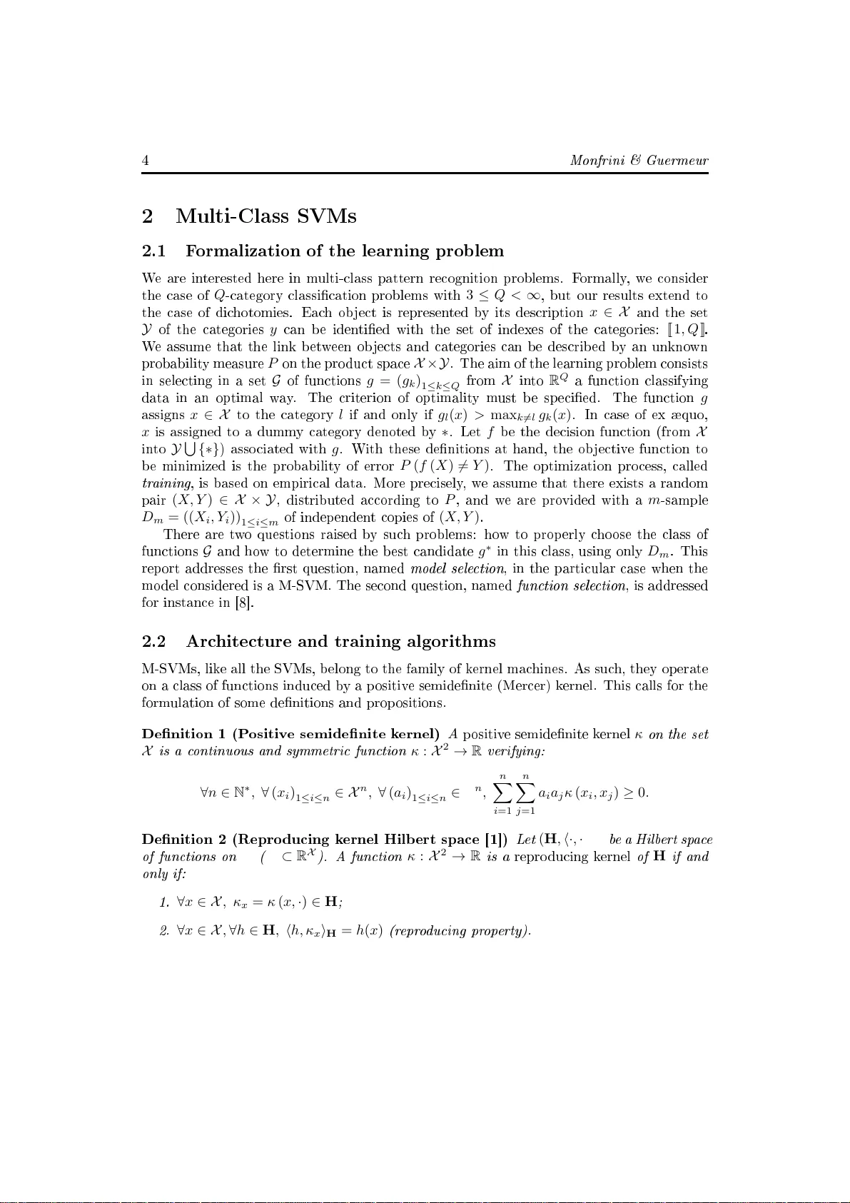
A Quadratic Loss Multi-Class SVM Emmanuel Monfrini — Y ann Guermeur November 1, 2021 A Quadrati Loss Multi-Class SVM Emman uel Monfrini ∗ , Y ann Guermeur † No v em b er 1, 2021 24 pages Abstrat: Using a supp ort v etor ma hine requires to set t w o t yp es of h yp erparameters: the soft margin parameter C and the parameters of the k ernel. T o p erform this mo del seletion task, the metho d of hoie is ross-v alidation. Its lea v e-one-out v arian t is kno wn to pro due an estimator of the generalization error whi h is almost un biased. Its ma jor dra wba k rests in its time requiremen t. T o o v erome this diult y , sev eral upp er b ounds on the lea v e-one-out error of the pattern reognition SVM ha v e b een deriv ed. Among those b ounds, the most p opular one is probably the radius-margin b ound. It applies to the hard margin pattern reognition SVM, and b y extension to the 2 -norm SVM. In this rep ort, w e in tro due a quadrati loss M-SVM, the M-SVM 2 , as a diret extension of the 2 -norm SVM to the m ulti-lass ase. F or this ma hine, a generalized radius-margin b ound is then established. Key-w ords: M-SVMs, mo del seletion, lea v e-one-out error, radius-margin b ound. ∗ UMR 7503-UHP † UMR 7503-CNRS Une SVM m ulti-lasse à oût quadratique Résumé : La mise en ÷uvre d'une ma hine à v eteurs supp ort requiert la détermination des v aleurs de deux t yp es d'h yp er-paramètres : le paramètre de marge doue C et les paramètres du no y au. P our eetuer ette tâ he de séletion de mo dèle, la métho de de hoix est la v alidation roisée. Sa v arian te lea v e-one-out est onn ue p our fournir un estimateur de l'erreur en généralisation presque sans biais. Son défaut premier réside dans le temps de alul qu'elle néessite. An de surmon ter ette diulté, plusieurs ma joran ts de l'erreur lea v e-one-out de la SVM alulan t des di hotomies on t été prop osés. La plus p opulaire de es b ornes sup érieures est probablemen t la b orne ra y on-marge. Elle s'applique à la v ersion à marge dure de la ma hine, et par extension à la v arian te dite de norne 2 . Ce rapp ort in tro duit une M-SVM à oût quadratique, la M-SVM 2 , omme une extension direte de la SVM de norne 2 au as m ulti-lasse. P our ette ma hine, une b orne ra y on-marge généralisée est ensuite établie. Mots-lés : M-SVM, séletion de mo dèle, erreur lea v e-one-out, b orne ra y on-marge. A Quadr ati L oss Multi-Class SVM 3 1 In tro dution Using a supp ort v etor ma hine (SVM) [2, 4 ℄ requires to set t w o t yp es of h yp erparameters: the soft margin parameter C and the parameters of the k ernel. T o p erform this mo del seletion task, sev eral approa hes are a v ailable (see for instane [9 , 12 ℄). The solution of hoie onsists in applying a ross-v alidation pro edure. Among those pro edures, the lea v e- one-out one app ears esp eially attrativ e, sine it is kno wn to pro due an estimator of the generalization error whi h is almost un biased [ 11 ℄. The seam y side of things is that it is highly time onsuming. This is the reason wh y , in reen t y ears, a n um b er of upp er b ounds on the lea v e-one-out error of pattern reognition SVMs ha v e b een prop osed in literature (see [3 ℄ for a surv ey). Among those b ounds, the tigh test one is the span b ound [16 ℄. Ho w ev er, the results of Chap elle and o-w ork ers presen ted in [3 ℄ sho w that another b ound, the radius- margin one [15 ℄, a hiev es equiv alen t p erformane for mo del seletion while b eing far simpler to ompute. This is the reason wh y it is urren tly the most p opular b ound. It applies to the hard margin ma hine and, b y extension, to the 2 -norm SVM (see for instane Chapter 7 in [13 ℄). In this rep ort, a m ulti-lass extension of the 2 -norm SVM is in tro dued. This ma hine, named M-SVM 2 , is a quadrati loss m ulti-lass SVM, i.e., a m ulti-lass SVM (M-SVM) in whi h the ℓ 1 -norm on the v etor of sla k v ariables has b een replaed with a quadrati form. The standard M-SVM on whi h it is based is the one of Lee, Lin and W ah ba [10 ℄. As the 2 -norm SVM, its training algorithm is equiv alen t to the training algorithm of a hard margin ma hine obtained b y a simple hange of k ernel. W e then establish a generalized radius- margin b ound on the lea v e-one-out error of the hard margin v ersion of the M-SVM of Lee, Lin and W ah ba. The organization of this pap er is as follo ws. Setion 2 presen ts the m ulti-lass SVMs, b y desribing their ommon ar hiteture and the general form tak en b y their dieren t training algorithms. It fo uses on the M-SVM of Lee, Lin and W ah ba. In Setion 3, the M-SVM 2 is in tro dued as a partiular ase of quadrati loss M-SVM. Its onnetion with the hard margin v ersion of the M-SVM of Lee, Lin and W ah ba is highligh ted, as w ell as the fat that it onstitutes a m ulti-lass generalization of the 2 -norm SVM. Setion 4 is dev oted to the form ulation and pro of of the orresp onding m ulti-lass radius-margin b ound. A t last, w e dra w onlusions and outline our ongoing resear h in Setion 5. 4 Monfrini & Guermeur 2 Multi-Class SVMs 2.1 F ormalization of the learning problem W e are in terested here in m ulti-lass pattern reognition problems. F ormally , w e onsider the ase of Q -ategory lassiation problems with 3 ≤ Q < ∞ , but our results extend to the ase of di hotomies. Ea h ob jet is represen ted b y its desription x ∈ X and the set Y of the ategories y an b e iden tied with the set of indexes of the ategories: [ [ 1 , Q ] ] . W e assume that the link b et w een ob jets and ategories an b e desrib ed b y an unkno wn probabilit y measure P on the pro dut spae X × Y . The aim of the learning problem onsists in seleting in a set G of funtions g = ( g k ) 1 ≤ k ≤ Q from X in to R Q a funtion lassifying data in an optimal w a y . The riterion of optimalit y m ust b e sp eied. The funtion g assigns x ∈ X to the ategory l if and only if g l ( x ) > max k 6 = l g k ( x ) . In ase of ex æquo, x is assigned to a dumm y ategory denoted b y ∗ . Let f b e the deision funtion (from X in to Y S {∗} ) asso iated with g . With these denitions at hand, the ob jetiv e funtion to b e minimized is the probabilit y of error P ( f ( X ) 6 = Y ) . The optimization pro ess, alled tr aining , is based on empirial data. More preisely , w e assume that there exists a random pair ( X, Y ) ∈ X × Y , distributed aording to P , and w e are pro vided with a m -sample D m = (( X i , Y i )) 1 ≤ i ≤ m of indep enden t opies of ( X, Y ) . There are t w o questions raised b y su h problems: ho w to prop erly ho ose the lass of funtions G and ho w to determine the b est andidate g ∗ in this lass, using only D m . This rep ort addresses the rst question, named mo del sele tion , in the partiular ase when the mo del onsidered is a M-SVM. The seond question, named funtion sele tion , is addressed for instane in [8 ℄. 2.2 Ar hiteture and training algorithms M-SVMs, lik e all the SVMs, b elong to the family of k ernel ma hines. As su h, they op erate on a lass of funtions indued b y a p ositiv e semidenite (Merer) k ernel. This alls for the form ulation of some denitions and prop ositions. Denition 1 (P ositiv e semidenite k ernel) A p ositiv e semidenite k ernel κ on the set X is a ontinuous and symmetri funtion κ : X 2 → R verifying: ∀ n ∈ N ∗ , ∀ ( x i ) 1 ≤ i ≤ n ∈ X n , ∀ ( a i ) 1 ≤ i ≤ n ∈ R n , n X i =1 n X j =1 a i a j κ ( x i , x j ) ≥ 0 . Denition 2 (Repro duing k ernel Hilb ert spae [1 ℄) L et ( H , h· , ·i H ) b e a Hilb ert sp a e of funtions on X ( H ⊂ R X ). A funtion κ : X 2 → R is a repro duing k ernel of H if and only if: 1. ∀ x ∈ X , κ x = κ ( x, · ) ∈ H ; 2. ∀ x ∈ X , ∀ h ∈ H , h h, κ x i H = h ( x ) (r epr o duing pr op erty). A Quadr ati L oss Multi-Class SVM 5 A Hilb ert sp a e of funtions whih p ossesses a r epr o duing kernel is al le d a repro duing k ernel Hilb ert spae (RKHS). Prop osition 1 L et ( H κ , h· , ·i H κ ) b e a RKHS of funtions on X with r epr o duing kernel κ . Then, ther e exists a map Φ fr om X into a Hilb ert sp a e E Φ( X ) , h· , ·i suh that: ∀ ( x, x ′ ) ∈ X 2 , κ ( x, x ′ ) = h Φ ( x ) , Φ ( x ′ ) i . (1) Φ is al le d a feature map and E Φ( X ) a feature spae . The onnetion b et w een p ositiv e semidenite k ernels and RKHS is the follo wing. Prop osition 2 If κ is a p ositive semidenite kernel on X , then ther e exists a RKHS ( H , h· , ·i H ) of funtions on X suh that κ is a r epr o duing kernel of H . Let κ b e a p ositiv e semidenite k ernel on X and let ( H κ , h· , ·i H κ ) b e the RKHS spanned b y κ . Let ¯ H = ( H κ , h· , ·i H κ ) Q and let H = (( H κ , h· , ·i H κ ) + { 1 } ) Q . By onstrution, H is the lass of v etor-v alued funtions h = ( h k ) 1 ≤ k ≤ Q on X su h that h ( · ) = m k X i =1 β ik κ ( x ik , · ) + b k ! 1 ≤ k ≤ Q where the x ik are elemen ts of X , as w ell as the limits of these funtions when the sets { x ik : 1 ≤ i ≤ m k } b eome dense in X in the norm indued b y the dot pro dut (see for instane [17 ℄). Due to Equation 1, H an b e seen as a m ultiv ariate ane mo del on Φ ( X ) . F untions h an then b e rewritten as: h ( · ) = ( h w k , ·i + b k ) 1 ≤ k ≤ Q where the v etors w k are elemen ts of E Φ( X ) . They are th us desrib ed b y the pair ( w , b ) with w = ( w k ) 1 ≤ k ≤ Q ∈ E Q Φ( X ) and b = ( b k ) 1 ≤ k ≤ Q ∈ R Q . As a onsequene, ¯ H an b e seen as a m ultiv ariate linear mo del on Φ ( X ) , endo w ed with a norm k . k ¯ H giv en b y: ∀ ¯ h ∈ ¯ H , ¯ h ¯ H = v u u t Q X k =1 k w k k 2 = k w k , where k w k k = p h w k , w k i . With these denitions and prop ositions at hand, a generi denition of the M-SVMs an b e form ulated as follo ws. Denition 3 (M-SVM, Denition 42 in [ 8 ℄) L et (( x i , y i )) 1 ≤ i ≤ m ∈ ( X × [ [ 1 , Q ] ]) m and λ ∈ R ∗ + . A Q -ategory M-SVM is a lar ge mar gin disriminant mo del obtaine d by minimizing over the hyp erplane P Q k =1 h k = 0 of H a p enalize d risk J M-SVM of the form: J M-SVM ( h ) = m X i =1 ℓ M-SVM ( y i , h ( x i )) + λ ¯ h 2 ¯ H wher e the data t omp onent involves a loss funtion ℓ M-SVM whih is onvex. 6 Monfrini & Guermeur Three main mo dels of M-SVMs an b e found in literature. The oldest one is the mo del of W eston and W atkins [ 19 ℄, whi h orresp onds to the loss funtion ℓ WW giv en b y: ℓ WW ( y , h ( x )) = X k 6 = y (1 − h y ( x ) + h k ( x )) + , where the hinge loss funtion ( · ) + is the funtion max(0 , · ) . The seond one is due to Crammer and Singer [5℄ and orresp onds to the loss funtion ℓ CS giv en b y: ℓ CS ( y , ¯ h ( x )) = 1 − ¯ h y ( x ) + max k 6 = y ¯ h k ( x ) + . The most reen t mo del is the one of Lee, Lin and W ah ba [10 ℄ whi h orresp onds to the loss funtion ℓ LL W giv en b y: ℓ LL W ( y , h ( x )) = X k 6 = y h k ( x ) + 1 Q − 1 + . (2) Among the three mo dels, the M-SVM of Lee, Lin and W ah ba is the only one that implemen ts asymptotially the Ba y es deision rule. It is Fisher onsistent [ 20 , 14 ℄. 2.3 The M-SVM of Lee, Lin and W ah ba The substitution in Denition 3 of ℓ M-SVM with the expression of the loss funtion ℓ LL W giv en b y Equation 2 pro vides us with the expressions of the quadrati programming (QP) problems orresp onding to the training algorithms of the hard margin and soft margin v ersions of the M-SVM of Lee, Lin and W ah ba. Problem 1 (Hard margin M-SVM) min w , b J HM ( w , b ) s.t. h w k , Φ( x i ) i + b k ≤ − 1 Q − 1 , (1 ≤ i ≤ m ) , (1 ≤ k 6 = y i ≤ Q ) P Q k =1 w k = 0 P Q k =1 b k = 0 wher e J HM ( w , b ) = 1 2 Q X k =1 k w k k 2 . Problem 2 (Soft margin M-SVM) min w , b J SM ( w , b ) A Quadr ati L oss Multi-Class SVM 7 s.t. h w k , Φ( x i ) i + b k ≤ − 1 Q − 1 + ξ ik , (1 ≤ i ≤ m ) , (1 ≤ k 6 = y i ≤ Q ) ξ ik ≥ 0 , (1 ≤ i ≤ m ) , (1 ≤ k 6 = y i ≤ Q ) P Q k =1 w k = 0 P Q k =1 b k = 0 wher e J SM ( w , b ) = 1 2 Q X k =1 k w k k 2 + C m X i =1 X k 6 = y i ξ ik . In Problem 2, the ξ ik are slak variables in tro dued in order to relax the onstrain ts of orret lassiation. The o eien t C , whi h haraterizes the trade-o b et w een predition auray on the training set and smo othness of the solution, an b e expressed in terms of the regularization o eien t λ as follo ws: C = (2 λ ) − 1 . It is alled the soft mar gin p ar ameter . Instead of diretly solving Problems 1 and 2 , one usually solv es their W olfe dual [ 6℄. W e no w deriv e the dual problem of Problem 1. Giving the details of the implemen tation of the Lagrangian dualit y will pro vide us with partial results whi h will pro v e useful in the sequel. Let α = ( α ik ) 1 ≤ i ≤ m, 1 ≤ k ≤ Q ∈ R Qm + b e the v etor of Lagrange m ultipliers asso iated with the onstrain ts of go o d lassiation. It is for on v eniene of notation that this v e- tor is expressed with double subsript and that the dumm y v ariables α iy i , all equal to 0 , are in tro dued. Let δ ∈ E Φ( X ) b e the Lagrange m ultiplier asso iated with the onstrain t P Q k =1 w k = 0 and β ∈ R the Lagrange m ultiplier asso iated with the onstrain t P Q k =1 b k = 0 . The Lagrangian funtion of Problem 1 is giv en b y: L ( w , b , α, β , δ ) = 1 2 Q X k =1 k w k k 2 − h δ, Q X k =1 w k i − β Q X k =1 b k + m X i =1 Q X k =1 α ik h w k , Φ( x i ) i + b k + 1 Q − 1 . (3) Setting the gradien t of the Lagrangian funtion with resp et to w k equal to the n ull v etor pro vides us with Q alternativ e expressions for the optimal v alue of v etor δ : δ ∗ = w ∗ k + m X i =1 α ∗ ik Φ( x i ) , (1 ≤ k ≤ Q ) . (4) Sine b y h yp othesis, P Q k =1 w ∗ k = 0 , summing o v er the index k pro vides us with the expression of δ ∗ as a funtion of dual v ariables only: δ ∗ = 1 Q m X i =1 Q X k =1 α ∗ ik Φ( x i ) . (5) 8 Monfrini & Guermeur By substitution in to ( 4), w e get the expression of the v etors w k at the optim um: w ∗ k = 1 Q m X i =1 Q X l =1 α ∗ il Φ( x i ) − m X i =1 α ∗ ik Φ( x i ) , (1 ≤ k ≤ Q ) whi h an also b e written as w ∗ k = m X i =1 Q X l =1 α ∗ il 1 Q − δ k,l Φ( x i ) , (1 ≤ k ≤ Q ) (6) where δ is the Krone k er sym b ol. Let us no w set the gradien t of (3) with resp et to b equal to the n ull v etor. It omes: β ∗ = m X i =1 α ∗ ik , (1 ≤ k ≤ Q ) and th us m X i =1 Q X l =1 α ∗ il 1 Q − δ k,l = 0 , (1 ≤ k ≤ Q ) . Giv en the onstrain t P Q k =1 b k = 0 , this implies that: m X i =1 Q X k =1 α ∗ ik b ∗ k = β ∗ Q X k =1 b ∗ k = 0 . (7) By appliation of (6), Q X k =1 k w ∗ k k 2 = Q X k =1 h m X i =1 Q X l =1 α ∗ il 1 Q − δ k,l Φ( x i ) , m X j =1 Q X n =1 α ∗ j n 1 Q − δ k,n Φ( x j ) i = m X i =1 m X j =1 Q X l =1 Q X n =1 α ∗ il α ∗ j n h Φ( x i ) , Φ( x j ) i Q X k =1 1 Q − δ k,l 1 Q − δ k,n = m X i =1 m X j =1 Q X l =1 Q X n =1 α ∗ il α ∗ j n δ l,n − 1 Q κ ( x i , x j ) . (8) Still b y appliation of (6 ), m X i =1 Q X k =1 α ∗ ik h w ∗ k , Φ( x i ) i = m X i =1 Q X k =1 α ∗ ik h m X j =1 Q X l =1 α ∗ j l 1 Q − δ k,l Φ( x j ) , Φ( x i ) i A Quadr ati L oss Multi-Class SVM 9 = m X i =1 m X j =1 Q X k =1 Q X l =1 α ∗ ik α ∗ j l 1 Q − δ k,l κ ( x i , x j ) . (9) Com bining (8 ) and (9) giv es: 1 2 Q X k =1 k w ∗ k k 2 + m X i =1 Q X k =1 α ∗ ik h w ∗ k , Φ( x i ) i = − 1 2 Q X k =1 k w ∗ k k 2 = − 1 2 m X i =1 m X j =1 Q X k =1 Q X l =1 α ∗ ik α ∗ j l δ k,l − 1 Q κ ( x i , x j ) . (10) In what follo ws, w e use the notation e n to designate the v etor of R n su h that all its omp onen ts are equal to e . Let H b e the matrix of M Qm,Qm ( R ) of general term: h ik,j l = δ k,l − 1 Q κ ( x i , x j ) . With these notations at hand, rep orting (7) and (10 ) in (3 ) pro vides us with the algebrai expression of the Lagrangian funtion at the optim um: L ( α ∗ ) = − 1 2 α ∗ T H α ∗ + 1 Q − 1 1 T Qm α ∗ . This ev en tually pro vides us with the W olfe dual form ulation of Problem 1: Problem 3 (Hard margin M-SVM, dual form ulation) max α J LL W,d ( α ) s.t. ( α ik ≥ 0 , (1 ≤ i ≤ m ) , (1 ≤ k 6 = y i ≤ Q ) P m i =1 P Q l =1 α il 1 Q − δ k,l = 0 , (1 ≤ k ≤ Q ) wher e J LL W,d ( α ) = − 1 2 α T H α + 1 Q − 1 1 T Qm α, with the gener al term of the Hessian matrix H b eing h ik,j l = δ k,l − 1 Q κ ( x i , x j ) . Let the ouple w 0 , b 0 denote the optimal solution of Problem 1 and equiv alen tly , let α 0 = α 0 ik 1 ≤ i ≤ m, 1 ≤ k ≤ Q ∈ R Qm + b e the optimal solution of Problem 3. A ording to ( 6), the expression of w 0 k is then: w 0 k = m X i =1 Q X l =1 α 0 il 1 Q − δ k,l Φ( x i ) . 10 Monfrini & Guermeur 2.4 Geometrial margins F rom a geometrial p oin t of view, the algorithms desrib ed ab o v e tend to onstrut a set of h yp erplanes { ( w k , b k ) : 1 ≤ k ≤ Q } that maximize globally the C 2 Q mar gins b et w een the dieren ts ategories. If these margins are dened as in the bi-lass ase, their analytial expression is more omplex. Denition 4 (Geometrial margins, Denition 7 in [7 ℄) L et us onsider a Q - ate gory M-SVM (a funtion of H ) lassifying the examples of its tr aining set { ( x i , y i ) : 1 ≤ i ≤ m } without err or. γ kl , its margin b et w een ategories k and l , is dene d as the smal lest distan e of a p oint either in k or l to the hyp erplane sep ar ating those ate gories. L et us denote d M-SVM = min 1 ≤ k 0 . W e kno w that su h a mapping exists, otherwise, giv en the equalit y onstrain ts of Problem 3, v etor α p w ould b e equal to the n ull v etor. F or K 2 ∈ R ∗ + , let µ p b e the v etor of R Qm that only diers from the n ull v etor in the follo wing w a y: ( µ p pn = K 2 ∀ k ∈ [ [ 1 , Q ] ] \ { n } , µ p I ( k ) k = K 2 . Ob viously , this solution is feasible (satises the onstrain ts 17 ). Indeed, 1 Q P m i =1 P Q k =1 µ p ik = K 2 and P m i =1 µ p ik = K 2 , (1 ≤ k ≤ Q ) . With this denition of v etor µ p , the righ t-hand side of (23) simplies in to: K 2 h p n ( x p ) + X k 6 = n h p k x I ( k ) + Q Q − 1 . V etor µ p has b een sp eied so as to mak e it p ossible to exhibit a non trivial lo w er b ound on this last expression. By denition of n , h p n ( x p ) ≥ 0 . F urthermore, the Kuhn-T u k er optimalit y onditions: α p ik h w p k , Φ( x i ) i + b p k + 1 Q − 1 = 0 , (1 ≤ i 6 = p ≤ m ) , (1 ≤ k 6 = y i ≤ Q ) imply that h p k x I ( k ) 1 ≤ k 6 = n ≤ Q = − 1 Q − 1 1 Q − 1 . As a onsequene, a lo w er b ound on the righ t-hand side of ( 23 ) is pro vided b y: m X i =1 X k 6 = y i h p k ( x i ) + 1 Q − 1 µ p ik ≥ K 2 Q − 1 . It springs from this b ound and (22 ) that J ( α p + K 1 µ p ) − J ( α p ) ≥ K 1 K 2 Q − 1 − K 2 1 2 Q X k =1 m X i =1 Q X l =1 µ p il 1 Q − δ k,l Φ( x i ) 2 . (24) Com bining (18), (21 ) and (24 ) nally giv es: 1 2 Q X k =1 m X i =1 Q X l =1 λ p il 1 Q − δ k,l Φ( x i ) 2 ≥ A Quadr ati L oss Multi-Class SVM 19 K 1 K 2 Q − 1 − K 2 1 2 Q X k =1 m X i =1 Q X l =1 µ p il 1 Q − δ k,l Φ( x i ) 2 . (25) Let ν p = ( ν p ik ) 1 ≤ i ≤ m, 1 ≤ k ≤ Q b e the v etor of R Qm + su h that µ p = K 2 ν p . The v alue of the salar K 3 = K 1 K 2 maximizing the righ t-hand side of (25 ) is: K ∗ 3 = 1 Q − 1 P Q k =1 P m i =1 P Q l =1 ν p il 1 Q − δ k,l Φ( x i ) 2 . By substitution in ( 25 ), this means that: ( Q − 1 ) 2 Q X k =1 m X i =1 Q X l =1 λ p il 1 Q − δ k,l Φ( x i ) 2 Q X k =1 m X i =1 Q X l =1 ν p il 1 Q − δ k,l Φ( x i ) 2 ≥ 1 . F or η in R Qm , let K ( η ) = 1 Q P m i =1 P Q k =1 η p ik . W e ha v e: 1 Q m X i =1 Q X l =1 λ p il Φ( x i ) − m X i =1 λ p ik Φ( x i ) 2 = K ( λ p ) 2 k on v 1 (Φ( x i )) − on v 2 (Φ( x i )) k 2 where on v 1 (Φ( x i )) and on v 2 (Φ( x i )) are t w o on v ex om binations of the Φ( x i ) . As a onsequene, k on v 1 (Φ( x i )) − on v 2 (Φ( x i )) k 2 an b e b ounded from ab o v e b y D 2 m . Sine the same reasoning applies to ν p , w e get: ( Q − 1 ) 2 Q 2 K ( λ p ) 2 K ( ν p ) 2 D 4 m ≥ 1 . (26) By onstrution, K ( ν p ) = 1 . W e no w onstrut a v etor λ p minimizing the ob jetiv e funtion K . First, note that due to the equalit y onstrain ts satised b y this v etor, ∀ k ∈ [ [ 1 , Q ] ] , m X i =1 λ p ik = 1 Q m X i =1 Q X l =1 λ p il . As a onsequene, ∀ ( k , l ) ∈ [ [ 1 , Q ] ] 2 , m X i =1 λ p ik = m X i =1 λ p il . This implies that: ∀ k ∈ [ [ 1 , Q ] ] , m X i =1 λ p ik ≥ max l ∈ [ [ 1 ,Q ] ] α 0 pl . 20 Monfrini & Guermeur Ob viously , b oth the b o x onstrain ts in (16 ) and the nature of K all for the hoie of small v alues for the omp onen ts λ p ik . Th us, there is a feasible solution λ p ∗ su h that: ∀ k ∈ [ [ 1 , Q ] ] , m X i =1 λ p ik ∗ = max l ∈ [ [ 1 ,Q ] ] α 0 pl . This solution is su h that K ( λ p ∗ ) = max k ∈ [ [ 1 ,Q ] ] α 0 pk . The substitution of the v alues of K ( ν p ) and K ( λ p ∗ ) in (26) pro vides us with: max k ∈ [ [ 1 ,Q ] ] α 0 pk 2 ≥ 1 ( Q − 1) 2 Q 2 D 4 m . T aking the square ro ot of b oth sides onludes the pro of of the lemma. 4.3 Multi-lass radius-margin b ound Theorem 2 (Multi-lass radius-margin b ound) L et us onsider a Q - ate gory har d mar- gin M-SVM of L e e, Lin and W ahb a on a domain X . L et d m = { ( x i , y i ) : 1 ≤ i ≤ m } b e its tr aining set, L m the numb er of err ors r esulting fr om applying a le ave-one-out r oss-validation pr o e dur e to this mahine, and D m the diameter of the smal lest spher e of the fe atur e sp a e ontaining the set { Φ( x i ) : 1 ≤ i ≤ m } . Then the fol lowing upp er b ound holds true: L m ≤ Q 2 D 2 m X k
Original Paper
Loading high-quality paper...
Comments & Academic Discussion
Loading comments...
Leave a Comment