Simultaneous inference: When should hypothesis testing problems be combined?

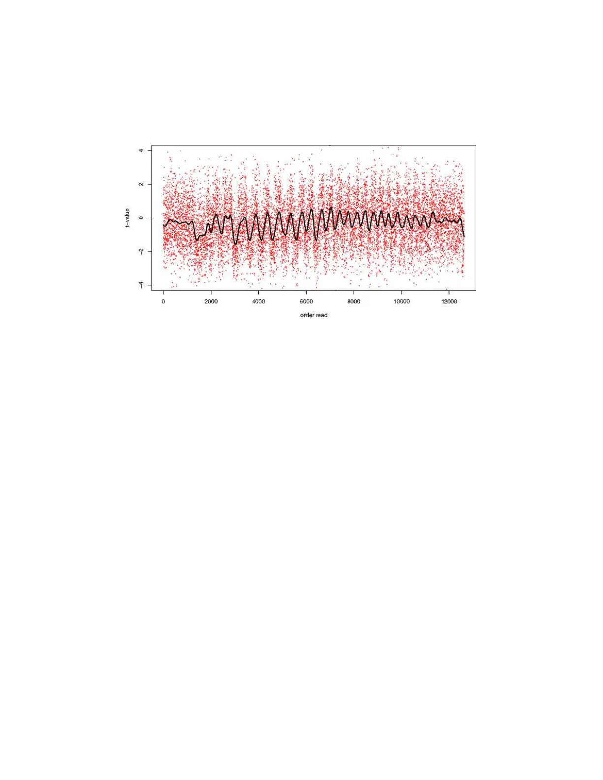
The Annals of Applie d Statistics 2008, V ol. 2, No. 1, 197–22 3 DOI: 10.1214 /07-A OAS141 c  Institute of Mathematical Statistics , 2008 SIMUL T ANEOUS INFERENCE: WHEN SHOULD HYPOTHESIS TESTING PR OBLEMS BE COMBINED? By Bradley Efron Stanfor d University Modern statisticia ns are often presented with hundreds or thou- sands of h yp othesis testing p roblems to eva luate at the same time, generated fro m new scien tific technolog ies suc h a s microarra ys, med- ical and satel lite i maging devices, or flow cytometry counters. The relev ant statistical literature tend s to b egin with the tacit assump- tion that a single combined analysis, for instance, a F alse Discov ery Rate assessmen t, should b e applied to the entire set of problems at hand. This can b e a dangerous assumption, as the ex amples in the pap er sho w, leading to ov erly conserv ativ e or ov erly liberal conclu- sions within any particular sub class of th e cases. A simple Bayes ian theory yields a succinct d escription of the effects of separation or com- bination on false disco very rate analyses. The theory allo ws efficient testing within small sub classes, and has applications to “en richment, ” the detection of m ulti-case effects. 1. In trod uction. Mo dern scien tific devices suc h as microarra ys routinely pro vide the statistic ian with thousands of hypothesis testing problems to consider at the same time. A v ariety of statistical tec hniques, f alse disco very rates, famil y-wise error rates, p erm u tatio n metho ds etc., ha ve b een prop osed to hand le large-scal e testing situations, usually u nder the tacit assump tion that all a v ailable tests sh ould b e analyzed together—for instance, emplo y- ing a single f alse disco very analysis for all the genes in a giv en microarray exp erimen t. This can b e a d angerous assu mption. As my examples will show, omnibus com bination may distort individu al inf erences in b oth d irect ions: h ighly sig- nifican t cases may b e hidden while insignifican t ones are enhanced. This pap er concerns the c hoice b et ween com bination and separation of hyp othe- sis testing problems. A h elpful m ethod ology will b e describ ed for diagnosing when separation ma y b e necessary for a subs et of the testing problems, as w ell as for carrying out separation in an efficien t f ashion. Received Ma y 2007; revised September 2007. Key wor ds and phr ases. F alse disco very rates, separate-class mo del, enrichmen t. This is an electronic reprint of the original article published b y the Institute of Mathematical Statistics in The Annals of Applie d Statistics , 2008, V ol. 2, No. 1, 197– 2 23 . This reprint differs from the o riginal in pa gination and t y pog r aphic detail. 1 2 B. EFRON Fig. 1. Br ain Data : z -values c omp aring 6 dyslexic childr en with 6 normals; horizontal se ction showing 848 of 15443 voxels. Co de: R e d z ≥ 0 , Gr e en z < 0 ; solid cir cles z ≥ 2 . 0 , solid squar es z ≤ − 2 . 0 ; “ x ” indic ates distanc e f r om b ack of br ain; y -axis is right-left distanc e. The fr ont half of the br ain app e ars to have mor e p ositive z -values. Data fr om Schwartzman, Doughert y and T aylor (2005) . Figure 1 illustrates our motiv ating example, tak en fr om Sc h w artzman, Doughert y and T a ylor (200 5) . Tw elve c hildr en, six dys lexic and six normal, receiv ed Diffusion T ensor Imaging (DTI) b rain scans, an adv anced form of MRI tec hnology that measures fluid diffusion in the brain, in this case at N = 15443 lo cations, eac h r epresen ted b y its o wn vo xel’s resp onse. A z -v alue “ z i ” comparing the dyslexics with the normals has b een calculated for eac h v oxel i , su c h that z i should hav e a standard normal distribution und er the n ull h yp othesis of no dyslexic-normal difference at that brain lo cation, the or etic al nul l hyp othesis : z i ∼ N (0 , 1) . (1.1) The z -v alues f or a h orizon tal section o f the b rain con taining 848 of the 15443 vo x els are in d icate d in Figure 1 . Distance “ x ” from the bac k tow ard the f ron t of the brain is indicated along the x axis. In app earance at least, the z i ’s seem to b e more p ositiv e to wa rd the front. The in vestig ators were, of course, in terested in s p otting lo cations of gen- uine br ain differences b et we en the dyslexic and normal c hildren. A standard F alse Disco v ery Rate (FDR) analysis describ ed in Section 2 , Benjamini and Ho c hberg (1995) , returned 198 “significan t” v o xels at thr eshold lev el q = 0 . 1, those havi ng z i ≥ 3 . 02. The histogram of all 15443 z i ’s app ears in the left panel of Figure 2 . Separate z -v alue histograms for the b ac k and fr ont h alv es of the brain are displa yed in the right panel of Figure 2 , with the dividing line at x = 49 . 5 SEP AR A TING AN D COMBININ G HY POTHESI S TESTS 3 Fig. 2. L eft p anel: hi sto gr am of al l 15433 z -values for Br ain Data; the 198 voxels with z i ≥ 3 . 02 wer e judge d signific ant by an FDR analysis with thr eshold level q = 0 . 1 . Right p anel: histo gr ams for b ack and fr ont voxels; sep ar ate FDR analyses at level q = 0.1 gave no signific ant voxels for b ack half, and 281 signific ant voxels, those with z i ≥ 2 . 69 , for fr ont half. MLE values ar e me ans and standar d deviations for normal densities fit to the c enters of the two histo gr ams, as explaine d in Se ction 3 . as sho w n in Figure 1 . Tw o discrepancies strik e the ey e: the hea vy righ t tail seen in the com b ined histogram on th e right comes almost exclusive ly from fron t-half vo xels; and the cent er of the back- half histogram is shifted left w ard ab out 0.35 u nits compared to the front . Separate FDR analyses, eac h at threshold lev el q = 0 . 1, w ere ru n on the bac k and fr on t half data. 281 fron t half v o xels were found significan t, those ha vin g z i ≥ 2 . 69; the bac k half analysis gav e no significant v oxel s at all, in con trast to 9 significan t bac k-half cases found in the com b ined analysis. This example illustrates b oth of the dangers of combinat ion—o ve r and u nder sensitivit y w ithin d ifferen t sub classes of the exp erimen t. Section 2 b egins with a simple Bay esian theorem that quan tifies the c hoice b et ween sep arate and com bined analysis. It is applied to the brain data in Section 3 , elucidating the d ifferences b et ween fron t and bac k f alse disco v- ery rate analyses. Th e theorem is most useful for separately inv estigating smal l sub classes, where there is too little d ata for the dir ect empirical Ba y es tec hniques of Section 3 . Sections 4 and 7 demonstrate how al l the data, all N = 15833 z v alues in the Brain study , can b e br ought to b ear on efficien t FDR estimation for a small sub class, for example, ju s t the 82 v o xels at dis- tance x = 18 . Section 6 applies small sub class theory to “enric h men t,” the assessmen t of a p ossible ov erall discrepancy b et ween the z -v alues w ithin and outside a c hosen class. 4 B. EFRON A reasonable ob jection to p erform ing separate analyses on p ortions of the N cases is the p ossibilit y of weak ening con trol of Typ e 1 err or, the ov erall size of the pro cedure. Th is qu estio n is tak en u p in Section 5 , where false disco very rate metho ds are sho wn to b e nearly imm u n e to the danger. Some tec hnical remarks and d iscussion end the pap er in Sections 8 and 9 . The question of separating large-scale testing problems has not r eceiv ed m u c h recen t atten tion. Two relev an t references are Geno v ese, Ro eder and W asserman (2006 ) , and F erkinstad, F rigessi, Thorleifsson and Kong (2007) . Enric hmen t tec hniques ha ve b een more activ ely dev elop ed, as in Su brama- nian et al. (2005 ) , Newton et al. (2007) and Efron and Tibshirani (2007) . 2. A separate-class mo del. The “Two- Groups mo del,” reviewe d b elo w, pro vides a simple Ba y esian fr amew ork for the analysis of sim ultaneous h y- p othesis testing problems. Th e framew ork will b e extended here to include the p ossibilit y of separate situations in differen t sub-classes of problems— for example, for the b ac k and front halv es of the b r ain in Figure 1 —the extended framew ork b eing the “Separate-Class mo del.” First, we b egin with a br ief r eview of the Tw o-Groups mo del, tak en from Efron ( 2005 , 2007a ). It starts with the Ba y esian assump tion that eac h of the N cases (all N = 15443 vo xels for the Brain Data) is either n u ll or nonnull, with pr ior probabilit y p 0 or p 1 = 1 − p 0 , and with its test statistic “ z ” ha ving densit y either f 0 ( z ) or f 1 ( z ), p 0 = Pr ob { n ull } , f 0 ( z ) density if null , (2.1) p 1 = Pr ob { nonn u ll } , f 1 ( z ) densit y if nonn ull . The theoretica l null mo d el ( 1.1 ) mak es f 0 ( z ) a standard normal densit y f 0 ( z ) = ϕ ( z ) = 1 √ 2 π e − 1 / 2 z 2 , (2.2) an assumption we will question more critically later. W e add the qualitativ e requiremen t that p 0 is large, s a y , p 0 ≥ 0 . 90 , (2.3) reflecting the usual purp ose of large-sca le testing, whic h is to reduce a v ast set of p ossibilities to a muc h smaller set of interesti ng pr osp ects. Mo del ( 2.1 ) is p articularly helpful f or motiv ating F alse Disco v ery Rate metho ds. Let F 0 ( z ) and F 1 ( z ) b e the cum ulativ e distribution functions (c.d.f.) corresp onding to f 0 ( z ) and f 1 ( z ), and define the mixture c.d.f. F ( z ) = p 0 F 0 ( z ) + p 1 F 1 ( z ) . (2.4) SEP AR A TING AN D COMBININ G HY POTHESI S TESTS 5 Then the a p osteriori probabilit y of a case b eing in the null group of ( 2.1 ), giv en that its z -v alue z i is less than some threshold z , is the “Ba yesia n false disco very rate” Fdr( z ) ≡ Pr ob { null | z i < z } = p 0 F 0 ( z ) /F ( z ) . (2.5) [It is notationally conv enien t here to consider the negativ e end of the z -scale, e.g., z = − 3, but w e could ju st as well tak e z i > z or | z i | > z in ( 2.5 ).] Benjamini and Ho ch b erg’s (1995 ) false disco very cont rol rule estimates Fdr( z ) by Fdr( z ) = p 0 F 0 ( z ) / ¯ F ( z ) , (2.6) where ¯ F ( z ) is th e empirical c.d.f. ¯ F ( z ) = # { z i ≤ z } / N . (2.7) Ha ving selected some cont rol lev el “ q ,” often q = 0 . 1, the rule declares all cases as nonnull ha ving z i ≤ z max , where z max is the maximum v alue of z satisfying Fdr( z max ) ≤ q . (2.8) [Usually taking p 0 = 1 and F 0 ( z ) the theoretical null c.d.f. Φ ( z ) in ( 2.5 ).] Rule ( 2.8 ), wh ic h lo oks Ba y esian here, can b e shown to h a v e an imp ortant frequen tist “con trol” prop erty: if the z i ’s are indep end ent, the exp ected p ro- p ortion of false disco veries, that is, the prop ortion of cases identified b y ( 2.8 ) that are actually from the null group in ( 2.1 ), will b e n o greater than q . Ben- jamini and Y ekutie li (2001 ) relax the indep endence r equiremen t somewhat. Most large-sca le testing situations exhibit substan tial correlations among the z v alues—ob vious in Figure 1 —bu t dep end en ce is less of a problem for the empirical Ba y es approac h to false d isco v ery rates w e will follo w here [see Efron ( 2007 a , (2007b) )]. Defining the mixtur e density f ( z ) from ( 2.1 ), f ( z ) = p 0 f 0 ( z ) + p 1 f 1 ( z ) (2.9) leads to the “local false disco v ery rate” fdr( z ), fdr( z ) ≡ Prob { n ull | z i = z } = p 0 f 0 ( z ) /f ( z ) (2.10) for the probabilit y of a case b eing in the null group giv en z -score z . Densities are more natural than the tail areas of ( 2.5 ) for Ba y esian analysis. Both will b e used in w hat follo w s. The Sep ar ate-Class mo del extends ( 2.1 ) to co ver the situation wh ere the N cases can b e divided into distinct classes, p ossibly h a ving differen t c hoices of p 0 , f 0 and f 1 . Figure 3 illustrates the sc h eme: the tw o classes “A” and “B” (fron t and bac k in Figure 2 ) ha ve a priori probabilities π A and π B = 1 − π A . 6 B. EFRON Fig. 3. A Sep ar ate-Class m o del with two classes : The N c ases sep ar ate into classes A or B with a priori pr ob abili ty π A or π B ; the Two-Gr oups mo del ( 2.1 ) holds sep ar ately, with p ossibly differ ent p ar am eters, within e ach class. The Two-Groups m od el ( 2.1 ) holds separately within eac h class, for example, with p 0 = p A 0 , f 0 ( z ) = f A 0 ( z ), and f 1 ( z ) = f A 1 ( z ) in class A. I t is imp ortant to notice that the class lab el, A or B, is observ ed b y the statistician, in con trast to the n u ll/nonnull dichoto m y , which must b e inferred. Our pr evious definitions app ly separately to classes A an d B, for instance, follo wing ( 2.9 )–( 2.10 ), f A ( z ) = p A 0 f A 0 ( z ) + p A 1 f A 1 ( z ) and (2.11) fdr A ( z ) = p A 0 f A 0 ( z ) /f A ( z ) . Com b ining the tw o classes in Figure 3 giv es m arginal den s ities f 0 ( z ) = π A f A 0 ( z ) + π B f B 0 ( z ) , (2.12) f 1 ( z ) = π A f A 1 ( z ) + π B f B 1 ( z ) , and p 0 = π A p A 0 + π B p B 0 , s o f ( z ) = π A f A ( z ) + π B f B ( z ) , (2.13) leading to the com bin ed lo cal false disco very rate fdr( z ) = p 0 f 0 ( z ) /f ( z ) as in ( 2.10 ). Th e same relationships with c.d.f.’s replacing den s ities apply to tail area Fdr’s, ( 2.5 ). Ba ye s theorem yields a simp le but useful relationship b etw een the separate and com bined false disco v ery rates: Theorem. Define π A ( z ) as the c onditional pr ob ability of class A give n z , π A ( z ) = Prob { A | z } , (2.14) SEP AR A TING AN D COMBININ G HY POTHESI S TESTS 7 and also π A 0 ( z ) = Prob 0 { A | z } , (2.15) the c onditional pr ob ability of class A given z for a nul l c ase. Then fdr A ( z ) = fdr( z ) · π A 0 ( z ) π A ( z ) . (2.16) Pr oof. Let I b e the even t that a case is n ull, so I occurs in the tw o n ull paths of Figure 3 but n ot otherwise. Th en , from definition ( 2.10 ), fdr A ( z ) fdr( z ) = Prob { I | A, z } Prob { I | z } = Prob { I , A | z } Prob { A | z } Prob { I | z } (2.17) = Prob { A | I , z } Prob { A | z } = π A 0 ( z ) π A ( z ) .  The Theorem has u seful practical applications. Section 4 sho ws that the ratio R A ( z ) = π A 0 ( z ) /π A ( z ) (2.18) in ( 2.16 ) can often b e easily estimated, yielding helpful diagnostic s for p os- sible discrepancies b etw een fd r A ( z ) and f dr( z ), the separate and com bin ed false disco ve ry rates. T ail-area false disco v ery r ates ( 2.5 ) also follo w ( 2.16 ), after the ob vious definitional c hanges, Fdr A ( z ) = Fdr( z ) · R A ( z ) , (2.19) where no w R A ( z ) in volv es pr obab ilities for cases ha ving z i ≤ z , R A ( z ) = Prob 0 { A | z i ≤ z } Prob { A | z i ≤ z } . (2.20) There is no r eal reason, except exp ositional clarit y , for restricting atten- tion to jus t tw o classes. Section 4 briefly discusses versions of the Theorem applicable to more nuanced situations—in terms of Figure 1 , for example, where the relev ance of other cases to the fdr at a giv en “ x ” falls off smo othly as we mo v e aw a y from x . First though, Section 3 applies the Theorem to the dic h otomo us front-bac k Brain Data analysis. 3. Class-wise Fd r estimation. Th e Theorem of Section 2 sa ys that sep- arate and com bined lo cal false disco very rates are related by fdr A ( z ) = fdr( z ) · R A ( z ) , R A ( z ) = π A 0 ( z ) /π A ( z ) , (3.1) where π A 0 ( z ) and π A ( z ) are the conditional p robabilities Pr ob 0 { A | z } and Prob { A | z } . This section applies ( 3.1 ) to the Brain Data of Figures 1 and 2 , 8 B. EFRON Fig. 4. Points ar e pr op ortion of fr ont-half voxels r Ak , ( 3.2 ) , for Br ain Data of Figur e 2 . Solid curve i s b π A ( z ) , cubic lo gistic r e gr ession estimate of π A ( z ) = Prob { A | z } ; Dashe d curve b π A 0 ( z ) estimates Prob 0 { A | z } as explaine d i n text. taking the front-half v oxe ls as class A. Th e f ron t-bac k dic hotom y is extended to a more realistic multi-cl ass mo del in Section 4 . In ord er to estimate π A ( z ), it is conv enien t, though not n ecessary , to bin the z -v alues. Define r Ak as the p rop ortion of class A z -v alues in bin k , r Ak = N Ak / N k , (3.2) with N k the num b er of z i ’s ob s erved in b in k , and N Ak the num b er of those originating from v oxe ls in class A. The p oin ts in Figure 4 sho w r Ak for K = 42 b ins, eac h of length 0.2, runn ing from z = − 4 . 2 to 4.2. As suggested b y the right p anel of Figure 2 , the prop ortions r Ak steadily increase as w e mo ve from left to right. A standard weigh ted logist ic regression, fitting logit( π Ak ) as a cubic fu nc- tion of midp oint z ( k ) of bin k , w ith wei gh ts N k , yielded estimate b π A ( z ) sho w n by the solid curv e in Figure 4 . Binn ing isn ’t necessary here, but it is comforting to see b π A ( z ) n icely follo wing the r Ak p oin ts. (The three bins with r Ak = 0 at the extreme left con tain only N k = 2 z i ’s eac h.) In order to estimate π A 0 ( z ), we need to m ak e some assumptions ab out the null d istributions in the Tw o-Class mo del of Figure 3 . F ollo wing Ef ron ( 2004a , 2004b ), we assume that f A 0 ( z ) and f B 0 ( z ) are normal densities, but not necessarily N (0 , 1) as in ( 1.1 ), sa y , f A 0 ( z ) ∼ N ( δ A 0 , σ 2 A 0 ) and f B 0 ( z ) ∼ N ( δ B 0 , σ 2 B 0 ) . (3.3) Ba ye s theorem then giv es π A 0 ( z ) π B 0 ( z ) = π A 0 ( z ) 1 − π A 0 ( z ) SEP AR A TING AN D COMBININ G HY POTHESI S TESTS 9 T able 1 Par ameter estimates for the nul l arms of the Two-Class mo del in Figur e 3 , br ain data. Obtaine d using R pr o gr am l o cfdr, Efr on (2007b) , MLE fitting metho d b p 0 b δ 0 b σ 0 π A (front): 0.97 0.06 1.09 0.50 B (back): 1.00 − 0 . 29 1.01 0.50 (3.4) = π A p A 0 σ B 0 π B p B 0 σ A 0 exp  − 0 . 5  z − δ A 0 σ A 0  2 −  z − δ B 0 σ B 0  2  , whic h is easily solv ed for π A 0 ( z ). The R alg orithm lo cf dr used “MLE fitting” d escrib ed in Section 4 of Efron (2007 b) to pr o vide th e p arameter estimates in T able 1 . (The front- bac k dividin g line in Figure 1 wa s chosen to put ab out h alf the vo xels in to eac h class, so π A /π B . = 1 .) Solving f or b π A 0 in ( 3.4 ) ga ve the dashed cur v e of Figure 4 . Lo oking at Figure 2 , we migh t exp ect fdr A ( z ), the local fdr for the fr ont, to b e muc h low er than the com bined fdr( z ) for large v alues of z , that is, to pro vide man y m ore “significan t” z -v alues, but this is not the case: in fact, b R A ( z ) = b π A 0 ( z ) / b π A ( z ) . = 0 . 94 (3.5) for z ≥ 3 . 0, so form ula ( 3.1 ) imp lies only small differences. T w o con tradictory effects are at work: the longer right tail of th e fron t-half d istribution b y itself w ould pr od uce small v alues of R A ( z ) and fdr A ( z ); ho w ev er, th is effect is mostly canceled by the right w ard shift of the whole f r on t-half distrib ution, whic h s ubstan tially increases th e numerator of fdr A ( z ) = p A 0 f A 0 ( z ) /f A ( z ), ( 2.11 ). [Note: th e “significan t” vo xels in Figure 2 w ere obtained using the theoretica l null ( 1.1 ) for b oth the separate and com bined analyses, making them somewh at differen t than those based on the empirical n ull estimates here.] The close matc h b etw een b π A 0 ( z ) and b π A ( z ) near z = 0 is no acciden t. F ollo wing through the definitions in Figure 3 and ( 2.11 ) give s, after a little rearrangemen t, π A ( z ) 1 − π A ( z ) = π A 0 ( z ) 1 − π A 0 ( z ) 1 + Q A ( z ) 1 + Q B ( z ) , (3.6) where Q A ( z ) = 1 − fdr A ( z ) fdr A ( z ) and Q B ( z ) = 1 − fdr B ( z ) fdr B ( z ) . (3.7) 10 B. EFRON Fig. 5. Br ain Data: z -values plotte d vertic al ly versus distanc e x fr om b ack of br ain. Smal l histo gr am shows x values for the 198 voxels wi th z i ≥ 3 . 02 , l eft p anel of Figur e 2 . Running p er c entile curves r eve al gener al upwar d shif t of z -values ne ar histo gr am mo de at x = 65 . Usually fd r A ( z ) and fdr B ( z ) will appro ximately equal 1.0 near z = 0, reflect- ing the large prep ond erance of null cases, (2.3), and the fact th at nonnull cases tend to pro duce z -v alues further a wa y from 0. Then (3.6) giv es π A ( z ) . = π A 0 ( z ) for z near 0 , (3.8) as seen in Figure 4 . Supp ose we b eliev e that f A 0 ( z ) = f B 0 ( z ) in Figure 3 , in other words, that the null cases are distrib uted ident ically in the tw o classes. [This b eing true, e.g., if we accept the theoretical null distribution ( 1.1 ), as is u sual in the microarra y literature.] Then π A 0 ( z ) will b e constan t as a fu nction of z , π A 0 ( z ) = π A p A 0 π A p A 0 + π B p B 0 = π A p A 0 p 0 . (3.9) Since b π A ( z ) in Figure 4 is not constan t near z = 0, and should closely ap- pro ximate π A 0 ( z ) there, we h av e evidence against f A 0 ( z ) = f B 0 ( z ) in this case, obtained without r ecourse to mo dels suc h as ( 3.3 ). 4. Fdr estimation f or small su b classes. Our d ivision of the Brain Data in to front and bac k halv es was somewhat arb itrary . Figure 5 sho ws the N = 15443 z -v alues plotted v ersus x , the distance fr om the bac k of the brain. A clear wa v e is visible, cresting n ear x = 65. Most of the 198 BH (0 . 1) significan t v oxels of Figure 2 o ccurred at the top of the crest. There is something worrisome h ere: th e z -v alues near x = 65 are s h ifted upw ard across their entire range, not just in th e upp er p ercen tiles. This SEP AR A TING AN D COMBININ G HY POTHESI S TESTS 11 Fig. 6. L eft p anel: Solid histo gr am shows 82 z -values for class A, the voxels at x = 18 ; Line histo gr am for al l other z -values in Br ain Data; “ cub ” i s cubic lo gistic r e gr ession estimate of 1 /R A ( z ) . R ight p anel: c ombine d lo c al false di sc overy r ate c fdr( z ) , obtain fr om lo cfdr algorithm, and c fdr A ( z ) = c fdr( z ) · b R A ( z ) . Dashes indic ate the 82 z i ’ s. migh t b e du e to a reading bias in the DTI imaging device, or a gen uine dif- ference b et w een d yslexic and normal children for al l b rain lo cati ons around x = 65. In neither case is it correct to assign some sp ecial significance to those v oxel s near x = 65 ha ving large z i scores. In fact, a separate Fdr analysis of the 1956 v o xels ha ving x in the range [60 , 69] [using lo cfdr to estimate their empirical n ull distribution as N (0 . 65 , 1 . 44 2 )] yielded no significan t cases. Figure 5 suggests that we migh t wish to p erform separate analyses on man y small su b classes of the data. Large classes can b e inv estigated directly , as ab ov e, but a fully sep arate analysis may b e to o muc h to ask for a su b class of less than a f ew hundred cases, as sho wn by the accuracy calculations of Efron (2007 b) . Relationship ( 3.1 ) can b e useful in s uc h situations. As an example, let class A b e the 82 v oxel s located at x = 18. These displa y some large z -v alues in Figure 5 , attained without the b enefit of riding a wa v e crest. Figure 6 shows their z -v alue histogram and a cub ic logistic regression estimate of π A ( z ) /π A , where π A = 82 / 1554 3 = 0 . 0053 . (4.1) This amoun ts to an estimate of 1 /R A ( z ) in ( 3.1 ). Here w e are assuming that A s h ares a common n ull distribu tion with all the other cases, f A 0 ( z ) = f B 0 ( z ) as in ( 3.9 ), a necessary assu mption sin ce th ere isn’t enough data in A to separately estimate π A 0 ( z ). In its fa vo r is the flatness of b π A ( z ) /π A near z = 0, a necessary d iagnost ic signal as discussed at the end of S ectio n 3 . [Remark 12 B. EFRON G of Section 8 discuss es replacing π A with π A 0 , ( 3.9 ), in the estimation of R A ( z ).] The r ight p anel of Figure 6 compares the com b ined lo cal false d isco v ery rate c fdr( z ), estimated using lo cfdr as in Efron ( 2007a ), with c fdr A ( z ) = c fdr( z ) · b R A ( z ) , (4.2) for z ≥ 0. The adjustment is subs tantia l. Whether or not it is gen u ine d e- p ends on the accuracy of b R A ( z ), as considered further in the “efficiency” discussion of Section 7 . So far we ha ve only discussed th e d ic hotomization of cases into t wo classes A and B of p ossibly separate r elev ance. Figure 5 might suggest a more con- tin u ous approac h in whic h the relev ance of case j to case i falls off smo othly as | x j − x i | in creases, for example, as 1 / (1 + | x j − x i | / 10). W e sup p ose that eac h case comprises three comp onents, case i = ( x i , I i , z i ) , (4.3) where x i is an observ able vec tor of co v ariates, I i is the unobserv able n ull indicator h aving I i = 1 or 0 as case i is from the null or nonnull group in ( 2.1 ), and z i is th e ob s erv able z -v alue. W e also d efine a “relev ance function” ρ i ( x ) taking v alues in the int erv al [0 , 1], whic h sa ys how relev an t a case w ith co v ariate x is to case i , the case of inte rest. [Previously , ρ i ( x j ) = 1 or 0 as x j w as or was not in the same class as x i .] The Two -Class mo del of Figure 3 can b e extended to a m u lti-cl ass mo d el, where eac h cov ariate v alue x h as its o wn distribu tion parameters p x 0 , f x 0 ( z ), and f x 1 ( z ), giving f x ( z ) = p x 0 f x 0 ( z ) + (1 − p x 0 ) f x 1 ( z ) and (4.4) fdr x ( z ) = p x 0 f x 0 ( z ) /f x ( z ) as in ( 2.11 ). Let fd r( z ) b e the com bined lo cal false disco very rate as in the Theorem of Section 2 , and fdr i ( z ) the separate rate fdr x i ( z ). Th en ( 3.1 ) generalize s to fdr i ( z ) = fdr( z ) · R i ( z ) , R i ( z ) = E 0 { ρ i ( x ) | z } E { ρ i ( x ) | z } , (4.5) “ E 0 ” indicating n ull case conditional exp ectati on. T ail area false disco very rates ( 2.5 ) also satisfy ( 4.5 ) after the r equisite definitional c hanges, Fdr i ( z ) = Fdr( z ) · R i ( z ) , R i ( z ) = E 0 { ρ i ( X ) | Z ≤ z } E { ρ i ( X ) | Z ≤ z } . (4.6) The emp irical v ersion of ( 4.6 ) clarifies its meaning. L et p j 0 and F j 0 ( z ) indicate p x 0 and the c.d.f. of f x 0 ( z ) for x = x j , ( 4.4 ), and let N ( z ) = # { z j ≤ SEP AR A TING AN D COMBININ G HY POTHESI S TESTS 13 z } . T aking account of all the different situations ( 4.3 ), the combined Fdr estimate ( 2.5 ) b ecomes Fdr( z ) = N X j =1 p j 0 F j 0 ( z ) / N ( z ) , (4.7) this b eing the ratio of exp ected null cases to observ ed total cases for z j ≤ z i . Similarly , Fdr i ( z ) = N X j =1 ρ i ( x j ) p j 0 F j 0 ( z ) . X z j ≤ z ρ i ( x j ) , (4.8) the ratio of exp ected n ull cases to total cases taking accoun t of the relev ance of x j to x i . Therefore, Fdr i ( z ) = Fdr( z ) · ¯ R i ( z ) , (4.9) ¯ R i ( z ) = [ P N j =1 ρ i ( x j ) p j 0 F j 0 ( z ) / P N j =1 p j 0 F j 0 ( z )] [ P z j ≤ z ρ i ( x j ) / N ( z )] ; the denominator of ¯ R i ( z ) is an ob vious estimate of E { ρ i ( X ) | Z ≤ z } in ( 4.6 ), while the n u m erator is the Ba yes estimate of E 0 { ρ i ( X ) | Z ≤ z } . 5. Are separate analyses legitimate ? The p rincipal, and sometimes only , concern of classical multi ple inference theory was the con trol of Typ e I error in sim ultaneous hyp othesis testing situations. T his r aises an imp ortan t qu es- tion: is it legitima te from an error con trol viewp oin t to sp lit su c h a s ituation in to separate analysis classes? The answ er, d iscussed b riefly here, dep ends up on the method of inference. The Bonferroni metho d applied to N indep endent hyp othesis tests rejects the n ull for those cases ha ving p -v alue p i sufficien tly small to accoun t for m u ltiplicit y , p i ≤ α/ N , (5.1) α = 0 . 05 b eing the familiar c hoice. If we n o w separate the cases into t w o classes of size N / 2, rejecting for p i ≤ α/ ( N/ 2), we effectiv ely double α . Some adjustmen t of Bonferroni’s metho d is necessary if we are con templat- ing separate analyses. Changing α to α/ 2 works here, but things get more complicate d f or situations su c h as those suggested by Figure 5 . F alse disco v ery rate metho d s are more f orgiving—usually they can b e applied to separate analyses in un c hanged form without u ndermining their inferen tial v alue. Basically , this is b ecause they are r ates , and, as s u c h, cor- rectly scale with “ N .” W e will discuss b oth Ba ye sian and f requen tist justi- fications for this state men t. 14 B. EFRON Starting in a Ba y esian framew ork, as in ( 4.3 ), let ( X, I , Z ) (5.2) represen t a random case, where X is an observ ed co v ariate v ector, I is an unobserve d ind icato r equaling 1 or 0 as the case is null or nonnull, and Z is the observ ed z -v alue. W e assume X has p rior distribution π ( x ). X might indicate class A or B in Figure 3 , or the distance from the bac k of the b rain in Figure 5 . Let Fdr x ( z ) b e the Ba y esian tail area false d isco v ery r ate ( 2.5 ) conditional on observing X = x , Fdr x ( z ) = Prob { I = 1 | X = x, Z ≤ z } . (5.3) (Remem b ering that we could ju st as wel l c hange the Z condition to Z ≥ z or | Z | ≤ z .) F or eac h x , d efine a threshold v alue z ( x ) by Fdr x ( z ( x )) = q (5.4 ) for some preselecte d control lev el q , p erhaps q = 0 . 10. This implies a rule R that mak es decisions “ b I ” according to ( 5.4 ), b I =  1 (null) , if Z > z ( X ), 0 (nonnull) , if Z ≤ z . (5.5) Rule R has a conditional Ba y esian false disco very r ate q for ev ery c hoice of x , Fdr x ( R ) ≡ Prob { I = 1 | b I = 0 , X = x } = q . (5 .6) Unconditionally , the rate is also q : Fdr( R ) = Pr ob { I = 1 | b I = 0 } = Z X Prob { I = 1 | Z ≤ z ( X ) , X = x } π ( x | Z ≤ z ) dx (5.7) = Z X q · π ( x | Z ≤ z ) dx = q . This verifies the Ba y esian separation pr op ert y f or false d isco v ery rates: Fdr x ( R ) = q separately for all x implies Fd r ( R ) = q . Separating the Fdr analyses has not weak ened the Fdr int erpretation for the en tire ensemble. F or an y fixed v alue of z , the combined Ba y esian false disco ve ry rate Fdr( z ) ( 2.5 ) is an a p osteriori mixtur e of the separate Fdr x ( z ) v alues, Fdr( z ) = Z X Fdr x ( z ) π ( x | Z ≤ z ) dx, (5.8) b y the same argument as in the top line of ( 5.7 ). Th ere will b e some thresh old v alue “ z (com b )” that make s Fdr( z (com b )) = q , (5.9) SEP AR A TING AN D COMBININ G HY POTHESI S TESTS 15 defining a combined d ecision rule R com b that, lik e R , con trols the Bay es false discov ery rate at q . Beca use of ( 5.8 ), z (com b ) will lie within the range of z ( X ); R com b will b e more or less conserv ativ e than the sep arated rule R as z (com b ) < z ( X ) or z (com b) > z ( X ) . 1 Not using the information in X reduces the theoretica l accuracy of rule R com b ; see Remark A of Section 8 . Result ( 5.7 ) justifies Fdr separation from a Ba yesian p oint of view. The corresp onding frequ entist/ empirical Ba y es calculat ions lead to essen tially the same conclusion, though n ot as cleanly as in ( 5.7 ). In order to justify the empir ical Ba y es in terpretation of Fdr( z ) ( 2.6 ), we w ould lik e it to accurately estimate Fdr( z ) ( 2.5 ). F ollo wing mo del ( 2.1 ), define N ( z ) = # { z i ≤ z } and e ( z ) = E { N ( z ) } = N · F ( z ); (5.10) also let D = Fdr( z ) Fdr( z ) and d = 1 − F ( z ) e ( z ) = 1 N 1 − F ( z ) F ( z ) . (5.11) Assuming indep endence of the z i (just for this calculat ion) standard bi- nomial results sho w that E { D } . = 1 + d a nd v ar { D } . = d, (5.12) where the appro ximations are acc urate to order O (1 / N ), ignoring terms O (1 / N 2 ). Remark B impro ves ( 5.12 ) to accuracy O (1 / N 2 ). W e see that Fdr( z ) is nearly unbiased for Fdr ( z ) with coefficient of v ari- ation CV( F dr ( z )) = d 1 / 2 ≤ e ( z ) − 1 / 2 . (5.13) W e n eed e ( z ) to b e reasonably large to make CV small enough for accurate estimatio n, p erhaps e ( z ) = N · F ( z ) ≥ 10 for CV ≤ 0 . 3 . (5.14) If we are w orking near the 1% tail of F ( z ), common enough in Fdr applica- tions, w e n eed N ≥ 1000. Making “ N ” as large as p ossible in th e b est reason for combined rather than separate analysis, at least in an empirical Ba ye s framew ork. The sepa- rate analyses s till ha v e large N ’s in the front -bac k example of Figure 2 , bu t 1 Geno vese , Ro eder and W asserman (2006) consider more qualitative situations where what we hav e called “A” or “B” migh t b e classes of greater or less a priori null probability . Their “w eighted BH” rule transforms z into v alues z A or z B dep ending u pon the class, and then carries out ru le ( 2.5 ) on th e transformed z ’s. Here, instead, the z ’s are kept the same, but compared to different thresholds z ( x ). F erkinstad et al. (2007) exp lore th e dep endence of Fdr( z ) on x via ex plicit p arametric mo dels. 16 B. EFRON not in Figure 6 . Section 7 sho ws ho w the small sub class approac h used in Section 4 can imp ro ve estimation efficiency . The danger of com bination is that we ma y b e gett ing a go od estimate of the wrong qu an tit y: if Fdr A ( z ) is m uc h d ifferen t than Fdr B ( z ), Fd r ( z ) ma y b e a p o or estimate of b oth. Returning to a com bin ed analysis, let N 0 ( z ) and N 1 ( z ) b e the num b er of n ull and n onn u ll z i ’s equal or less than z , for some fixed v alue of z , N o ( z ) = # { z i ≤ z , I i = 1 } and N 1 ( z ) = # { z i ≤ z , I i = 0 } (5.15) in notation ( 4.3 ), so N 0 ( z ) + N 1 ( z ) = N ( z ) , ( 5.10 ); also let e 0 ( z ) and e 1 ( z ) b e their exp ectations, e 0 ( z ) = E { N 0 ( z ) } = N p 0 · F 0 ( z ) and (5.16) e 1 ( z ) = E { N 1 ( z ) } = N p 1 · F 1 ( z ) . The ru le that declares b I i = 0 if z i ≤ z (i.e., “rejects th e n ull” for z i ≤ z ) has actual false disc overy pr op ortion Fdp( z ) = N 0 ( z ) N 0 ( z ) + N 1 ( z ) . (5.1 7) Fdp ( z ) is unobserv able, but w e can estimate it by Fdr( z ) ( 2.2 ), equaling e 0 ( z ) / ( N 0 ( z ) + N 1 ( z )) in notation ( 5.15 ). Th is is conserv ativ e in the fre- quen test sense of b eing an upw ardly biased estimate. I n fact, it is u p wardly biased giv en any fixed v alue of N 1 ( z ): E { Fdr( z ) | N 1 ( z ) } = E  e 0 ( z ) N 0 ( z ) + N 1 ( z )    N 1 ( z )  ≥ e 0 ( z ) e 0 ( z ) + N 1 ( z ) (5.18) ≥ E  N 0 ( z ) N 0 ( z ) + N 1 ( z )    N 1 ( z )  = E { Fdp( z ) | N 1 ( z ) } , where Jensen’s inequalit y has b een u sed t wice. On ly the definition E { N 0 ( z ) = e 0 ( z ) is requir ed here, not indep endent z i ’s. No w su p p ose we ha v e separated the cases into classes A and B, emplo y- ing separate rejection r ules z i ≤ z A and z i ≤ z B satisfying (in the ob vious notation) E { Fdr A ( z A ) } = E { Fdr B ( z B ) } ≡ q . (5.19) Applying ( 5.18 ) sh o ws that the separate false d isco v ery prop ortions will b e con trolled in exp ectation at r ate q . Ho wev er, for the equiv alen t of the SEP AR A TING AN D COMBININ G HY POTHESI S TESTS 17 Ba ye sian result ( 5.7 ) to hold fr equen tistically , we w an t the com bined F alse Disco v ery Prop ortion, Fdp com b = N A ( z A ) + N B 0 ( z B ) N A 0 ( z A ) + N B 0 ( z B ) + N A 1 ( z A ) + N B 1 ( z B ) , (5.20) to satisfy E { Fdp com b } ≤ q . Remarks C and D sho w that asymptotically E { Fdp com b } = q − c N + O (1 / N 2 ) (5.21) for some c ≥ 0, but an exact finite-sample result has not b een verified. (It fails if the d enominator exp ectat ions are v ery small.) Sim ulations sho w the original Benjamini–Hoch b erg rule b ehavi ng in the same wa y; app lying rule ( 2.8 ) s ep arately to classes A and B also con trols the ov erall exp ected v alue of Fdp com b at rate q , in the sense of ( 5.20 ). Bu t again this has n ot b een ve rified analytically . The conclusion of this section is that separate false disco v ery rates anal- yses are legimate, in th e sense that they do not inflate the com bin ed Fdr con trol rate, at least not if the d enominator exp ectations are reasonably large. 6. Enric hmen t calculations. Micro arra y stu dies fr equen tly yield disap- p oin ting results b ecause of low p o w er for detecting ind ividually s ignificant genes, Efr on ( 2007a ). “Enr ichmen t” tec hn iqu es strive for in creased p ow er b y p o oling the z -v alues from some pre-identified collec tion of genes, for in- stance, th ose from a sp ecified p ath wa y , as in S ubramanian et al. (2005 ) , Newton et al. (2007 ) and Efron and Tibsh irani (2007) . By thinking of the p o oled collectio n as “class A” in ( 2.16 ), the Th eorem of Section 2 can b e brought to b ear on enric hm ent an alysis. Figure 7 inv olv es a microarra y stud y of 10,100 genes, featured in Subrama- nian et al. (2005 ) , concerning transcription f actor, p 53. The stud y compared 17 normal cell lines with 33 lines exhibiting p53 m utations. T w o-sample t - tests yielded z -v alues z i for eac h gene, but the results were disapp oin ting: a standard Fdr test ( 2.8 ), with q = 0 . 1, yielded only one nonnull gene, “BAX.” The solid histogram in the left panel of Figure 7 sh o ws z i v alues for the 40 genes in set “P53 UP ,” a collection of genes kno wn to b e up -regulate d by gene p53. Compared with the line histogram of the 10,060 other z i ’s, the P53 UP set d efinitely lo oks “enric hed,” eve n though it con tains only one individually significan t z -v alue. The same analysis as in Figure 6 w as applied in Figure 7 , with class A no w the 40 P53 UP genes. Th e right panel sho w s d Fdr( z ) for the com bined analysis of all 10,10 0 genes [obtained from lo cfdr , using the theoretical n ull ( 1.1 )], and c fdr A ( z ) = c fdr( z ) · π A ˆ π A ( z ) , (6.1) 18 B. EFRON with π A = 40 / 1 0 , 100 as in (4.1) and ˆ π A ( z ) obtained from a cubic logistic regression. W e see that c fdr A ( z ) is m uc h smaller than c fdr( z ) for z ≥ 2. S ix of the P53 UP genes ha v e c fdr A ( z i ) < 0 . 10, now indicating strong evidence of b eing nonn u ll. The null hyp othesis of no enric hmen t can b e started as fdr A ( z ) = fdr( z ). Assuming π A 0 ( z ) constan t, as in ( 3.9 ), Theorem ( 2.16 ) pr o vides the equiv- alen t statemen t enrichment nul l hyp othesis : π A ( z ) = constan t , (6.2) so we can use π A ( z ) to test for enric hment. F or in stance, w e migh t estimate π A ( z ) with a linear logistic regression, and u se the test statistic S = ˆ β / c se, (6.3) where ˆ β is the estima ted regression slop e and c se its estimated standard error. F or the P53 UP gene set, ( 6.3 ) ga v e S = 4 . 54, t wo- sided p -v alue 6 . 10 − 6 . This agrees with the analyses in S u bramanian et al. and Efron and Tib- shirani, b oth of wh ic h judged P53 UP “enric hed ,” even taking accoun t of sim u ltaneous testing for sev eral hundred other gene s ets. (In situations lik e that of Figure 6 , where the class A z i ’s extend across a wide range of neg- ativ e and p ositiv e v alues, S should b e calculated sep arately for z < 0 and z > 0 ; in Figure 6 the p ositiv e z i ’s yielded S = 3 . 23 , p -v alue 0 . 001.) Fig. 7. p53 mi cr o arr ay study, 10,000 genes, c omp aring normal versus mutate d c el l lines. Solid histo gr am in left p anel shows z -values for 40 genes in class P53 UP, c omp ar e d with al l others ( line histo gr am ) . Right p anel c omp ar es c fdr( z ) for al l 10,000 genes wi th c fdr A ( z ) obtaine d as in (4.12). Six of the P53 UP genes have c fdr A ( z ) < 0 . 1 . SEP AR A TING AN D COMBININ G HY POTHESI S TESTS 19 Remark E connects ( 6.3 ) to more familiar enric hment test statistics, and suggests that it is like ly to b e reasonably efficien t. T he approac h here has one notable adv anta ge: w e obtain an assessment of individual s ignificance for the genes within the set, via c fdr A ( z i ) , rather than just an o v erall decision of enric h men t. 7. Efficiency . W e used the Theorem of S ection 2 to estimat e fdr A ( z ) for sub class A: c fdr A ( z ) = c fdr( z ) π A ˆ π A ( z ) , (7. 1) [setting π A 0 ( z ) in ( 2.6 ) equal to π A in Figures 6 and 7 ]. Of course, we could also estimate, fdr A ( z ) or the tail area analogue Fdr A ( z ), ( 2.19 ), directly from the class A d ata alone, but ( 7.1 ) is su bstan tially more efficien t. This section giv es a very brief o verview of the efficiency calculation, with Remark E of Section 8 pro viding a little more detail, concluding w ith a simulatio n example supp orting the accuracy of our metho dology . T aking loga rithms in ( 7.1 ) giv es log c fdr A ( z ) = log c fdr( z ) + log ˆ R A ( z ) , [ ˆ R A ( z ) = π A / ˆ π A ( z )] . (7.2) It tu r ns out th at log c fdr( z ) and log ˆ R A ( z ) are nearly un correlated with eac h other, leading to a conv enien t approximat ion for the standard deviation of log c fdr A ( z ): sd { log c fdr A ( z ) } = [( sd { log c fdr( z ) } ) 2 + ( sd { log ˆ R A ( z ) } ) 2 ] 1 / 2 . (7.3) Section 5 of Efron (2007b) p ro vides an accurate delta m ethod formula for sd { log c fdr( z ) } ; sd { log ˆ R A ( z ) } is also easy to approximat e, u sing familiar lo- gistic regression calcula tions. W e exp ect c fdr A ( z ) to b e more v ariable than c fdr( z ) since class A inv olv es only prop ortion π A of all N cases; standard sample-size considerations imply sd { log c fdr A ( z ) } ∼ 1 √ π A sd { log c fdr( z ) } (7.4) if c fdr A ( z ) and c fdr( z ) w ere estimated d irectly . E stimati on metho d ( 7.1 ) do es b etter—the extra v ariabilit y added to c fdr( z ) by ˆ R A ( z ) = π A / ˆ π A ( z ), repr e- sen ted by the last term in ( 7.3 ), tends to b e m u c h smaller than ( 7.4 ) suggests. Figure 8 illustrates a sim ulation example. In terms of the T w o-Class m o d el of Figure 3 , the p arameters are N = 5000 , π A = 0 . 01 , p A 0 = 0 . 5 , p B 0 = 1 . 0 (7.5) f A 0 = f B 0 ∼ N (0 , 1) and f A 1 = ∼ N (2 . 5 , 1) ; 20 B. EFRON Fig. 8. The thr e e standar d deviation terms of ( 7.3 ) for sim ul ation m o del ( 7.5 ) . so we exp ect 50 of the 5000 z i ’s to b e from class A, and 25 of these to b e nonnulls distributed as N ( 2 . 5 , 1), the remaining 4975 cases b eing N (0 , 1) n ulls. A t z = 2 . 5, the cen ter of the n onn u ll distribution, the ratio sd { log c fdr A ( z ) } /sd { log c fdr( z ) } is 1 . 61, compared to the ratio 10 suggested by ( 7.4 ). Similar results w ere obtained for other c hoices of the simulatio n parameters, ( 7.5 ). See Remark H . 8. Remarks. The remarks of this section expand on some of the tec hnical p oin ts raised earlier. Remark A ( Information loss if X is ignor e d ). The observed co v ariate X in (5.2), or x i in (4.3), is an ancillary statistic that affects the p osterior probabilit y of a null case, fdr x ( z ) = Prob { I = 1 | X = x, Z = z } . General prin - ciples say that ignoring X w ill increase prediction error f or I , and this can b e made pr ecise by considering sp ecific loss functions. Supp ose we wish to predict a binary v ariate I that equals 1 or 0 with probabilit y p or 1 − p ; f or a prediction “ P ” in (0 , 1), let the loss fu nction b e Q ( I , P ) = q ( P ) + ˙ q ( P )( I − P ) , (8.1) where q ( · ) is a p ositiv e conca ve fun ctio n on (0 , 1) satisfying q (0) = q (1) = 0 [e.g., q ( p ) = p · (1 − p ) or q ( p ) = − { p log( p ) + (1 − p ) log(1 − p ) } ], and ˙ q ( p ) = SEP AR A TING AN D COMBININ G HY POTHESI S TESTS 21 dq /dp . This is the “Q class” of loss fun ctio ns discussed in E f ron ( 2004a ). It then tur ns out that choosing P equal to the true probabilit y p minimizes exp ected loss, w ith risk E { Q ( I , p ) } = q ( p ). Giv en Z = z , the marginal false disco ve ry r ate is fdr( z ) = Prob { I = 1 | Z = z } = Z X fdr x ( z ) π ( x | z ) dx, (8.2) similar to ( 5.8 ). Th en, with fdr( z ) or fd r x ( z ) playi ng the r ole of the true probabilit y P , we hav e q (fdr( z )) = q  Z X fdr x ( z ) π ( x | z ) dx  ≥ Z X q (fdr x ( z )) π ( x | z ) dx (8. 3) b y Jensen’s inequalit y—in other wo rds, the u n conditional marginal risk q (fdr( z )) exceeds the exp ected risk conditioning on x . Remark B [ Co efficient of variation of Fdr( z )]. Standard calculatio ns in volving the first three momen ts of a binomial v ariate yield the mean and v ariance of D = Fdr( z ) / Fdr( z ), D ˙ ∼ (1 + d − d 2 c, d − d 2 (6 c − 1)) (8.4) for d = (1 − F ( z )) / ( N · F ( z )) as in ( 5.11 ), and c = (1 − 2 F ( z )) / (1 − F ( z )) , with errors O (1 / N 3 ). This giv es app ro ximate co efficien t of v ariation CV ( Fdr) . = d 1 / 2 [1 − d (3 c − 1 / 2)] , (8.5) impro ving on ( 5.1 3 ). Remark C ( Poisson mo del f or Fdr r elationship ). Let Z indicate some region of interest in the space of z -v alues for Figure 3 , for instance z ≤ z A in the A branc h and z ≤ z B in the B b ranc h. Denote th e n umber of null, nonnull, and total z i v alues in Z as N 0 ( Z ), N 1 ( Z ) and N ( Z ) = N 0 ( Z ) + N 1 ( Z ), with corresp onding exp ectations e 0 ( Z ), e 1 ( Z ) and e ( Z ) = e 0 ( Z ) + e 1 ( Z ). S ectio n 5 considers the relatio nship of three quanti ties, Fdr( Z ) = e 0 ( Z ) N ( Z ) , Fdr ( Z ) = e 0 ( Z ) e ( Z ) and Fdp( Z ) = N 0 ( Z ) N ( Z ) , (8.6) the estimated Benjamini–Hoch b erg FDR, the Ba yesia n Fdr and the F alse Disco v ery Prop ortion. No w assume th at N in Figure 3 is Poisson with exp ectation µ , and that the z i ’s are in dep enden t, N ∼ P oi( µ ) , z 1 , z 2 , . . . , z N indep endent, (8.7) implying that N 0 ( Z ) and N 1 ( Z ) are indep endent Poisson v ariates, N 0 ( Z ) ∼ P oi( e 0 ( Z )) indep end en t of N 1 ( Z ) ∼ P oi( e 1 ( Z )) . (8.8) 22 B. EFRON W e can write N 0 ( Z ) = e 0 ( Z ) + δ 0 , (8.9) where δ 0 has first three moments δ 0 ∼ (0 , e 0 ( Z ) , e 0 ( Z )) , (8.10) and similarly for N 1 ( Z ) ≡ e 1 ( Z ) + δ 1 and N ( Z ) ≡ e ( Z ) + δ . Note. The indep endence in ( 8.7 ) is not a necessary assum ption, but it leads to the neatly sp ecific forms of the relationship b elo w. The P oisson assum p tions make it easy to relate the t wo random quan tities Fdr( Z ) and Fdp( Z ) in ( 8.6 ) to th e p arameter Fdr ( Z ): Lemma. Under assumption ( 8.7 ), E { Fdr( Z ) } . = Fd r ( Z ) · (1 + 1 /e ( Z )) + O (1 /e ( Z ) 2 ) (8.11) and E { Fdp ( Z ) } . = Fd r( Z ) + O (1 /e ( Z ) 2 ) . (8.12) T ypic al ly, e ( Z ) = e 0 ( Z ) + e 1 ( Z ) wil l b e O ( µ ) , so that the err or terms in ( 8.11 )–( 8.12 ) ar e O (1 /µ 2 ) , eff e c tiv e ly O (1 / N 2 ) . The L e mma shows that Fdr ( Z ) , the Bayesian f alse disc overy r ate, is an exc el lent appr oximation to E { Fdp( Z ) } , while E { Fdr( Z ) } is only slightly upwar d ly biase d. Pr oof. F ollo wing through definitions ( 8.6 ) and ( 8.9 ), Fdr( Z ) − Fd r ( Z ) = e 0 ( Z ) e ( Z ) + δ − e 0 ( Z ) e ( Z ) = Fdr( Z )  1 1 + δ /e ( Z ) − 1  (8.13) . = Fdr( Z )  − δ e ( Z ) + δ 2 e ( Z ) 2  , so taking exp ecta tions yields ( 8.11 ). S imilarly , Fdr( Z ) − Fd p ( Z ) = Fdr( Z ) ·  1 − 1 + δ 0 /e 0 ( Z ) 1 + δ /e ( Z )  (8.14) . = Fdr( Z ) ·  1 −  1 + δ 0 e 0 ( Z )  1 − δ /e ( Z ) + δ 2 e ( Z ) 2  . SEP AR A TING AN D COMBININ G HY POTHESI S TESTS 23 Therefore, E { Fdr( Z ) − Fdp( Z ) } . = Fd r ( Z )  E  δ 0 δ e 0 ( Z ) e ( Z )  − E  δ 2 e ( Z ) 2  (8.15) = Fd r ( Z )  e 0 ( Z ) e 0 ( Z ) e ( Z ) − e ( Z ) e ( Z ) 2  = 0 .  Remark D ( F r e quentist Fdr c ombination r esult ). The Lemma ab o v e leads to a heuristic v erification of ( 5.21 ): that under ( 5.1 9 ), E { Fdr com b } ≤ q in ( 5.20 ). T o b egin w ith, notice that ( 8.7 ) giv es exp ected v alues of N A 0 ( z A ) and N A ( z A ), e A 0 ( z A ) = µπ A p A 0 F A 0 ( z A ) and e A ( z A ) = µπ A F A ( z A ) , (8.16) so e A 0 ( z A ) e A ( z A ) = p A 0 F A 0 ( z A ) F A ( z A ) = Fd r A ( z A ) , (8.17) the Ba ye sian Fdr for class A, and similarly , e B 0 ( z B ) /e B ( z B ) = Fdr B ( z B ). F rom ( 8.11 ) and ( 5.19 ), app lied individually w ithin the t wo classes, Fdr A ( z A ) . = q  1 − 1 e A ( z A )  ≤ q and (8.18) Fdr B ( z B ) . = q  1 − 1 e B ( z B )  ≤ q . Therefore, the com bined Ba y esian Fdr is also b ounded by q , Fdr com b = e A 0 ( z A ) + e B 0 ( z B ) e A ( z A ) + e B ( z B ) = e A ( z A ) Fdr A ( z A ) + e B ( z B ) Fdr B ( z B ) e A ( z A ) + e B ( z B ) (8.19) ≤ e A ( z A ) q + e B ( z B ) q e A ( z A ) + e B ( z B ) = q . But E { Fdp com b } . = Fd r com b according to ( 8.12 ), v erifyin g ( 5.21 ). Remark E ( Th e slop e statistic for testing enrichment ). Slop e statisti c ( 6.3 ), S = ˆ β / c se , is asymptotically fully efficien t f or enrichmen t testing un- der a tw o-sample exp onen tial families mo del. Sup p ose that all the z -v alues come, indep endently , from a one-paramete r exp onential family h a ving den- sit y functions g η ( z ) = e ηz − ψ ( η ) g 0 ( z ) , (8.20) 24 B. EFRON as in Lehmann and Romano (2005) , with η =  η A , in class A, η B , in class B. (8.21) Define β = η A − η B . As N → ∞ , the MLE ˆ β has asymp totic n ull hyp oth- esis distribution ˆ β ˙ ∼ N  β , 1 N π A π B V ( η 0 )  , (8.22) where π A and π B are the pr op ortions of z i ’s from the t wo classes, and V ( η 0 ) is the v ariance of z if η A = η B equals, sa y , η 0 . Ba ye s ru le applied to ( 8.20 )–( 8.21 ) giv es logit( π A ( z )) = β z + c  c = log  π A π B  + ψ ( η B ) − ψ ( η A )  , (8.23) with β = η A − η B as ab o v e. Standard calculations sho w that ˆ β obtained from the logistic regression mo del ( 8.23 ) also satisfies ( 8.22 ). Th is implies full asymptotic efficiency of th e slop e statistic ( 6.3 ) for testing η A = η B , the “no enric h m en t” n ull hypothesis. Under norm al assu m ptions, g η ( x ) ∼ N ( η , 1) in ( 8.20 ), ( 6.3 ) is asymptoticall y equiv alen t to z A − z B , the difference of class means; “limma” [Smyth (2004 ) ], an enrichmen t test implemen ted in Bio c onductor , is also based on z A , as discussed in Efron and Tibshirani (2007 b) . Remark F [ The additive varianc e appr oximation ( 7.3 )]. Being a little more careful, w e can use ( 3.9 ) to write ( 7.1 ) as c fdr A ( z ) = c fdr( z ) π A 0 ˆ π A ( z )  π A 0 = π A p A 0 π A p A 0 + π B p B 0  , (8.24) under the assum ption that f A 0 ( z ) = f B 0 ( z ) in Figure 3 . Binning the data as in ( 3.2 ) giv es ℓ c fdr Ak = ℓ c fdr k − ℓ ˆ π Ak + log( π A 0 ) , (8 .25) where ℓ c fdr Ak is log( c fdr A ( z )) ev aluated at the midp oin t z ( k ) of bin k , and sim- ilarly , ℓ c fdr k = log ( c fdr( z ( k ) )) and ℓ ˆ π Ak = log ( ˆ π A ( z ( k ) )). L o cfdr computes the estimates ℓ c fdr k from the vec tor of count s N = ( . . . , N k , . . . ), while a standard logistic regression program computes ℓ ˆ π Ak from th e vect or of prop ortions r A = ( . . . , r Ak = N Ak / N k , . . . ), ( 3.2 ); N and r A are, to a fi rst ord er of calcu- lation, uncorrelated, leading to appr o ximation ( 7.3 ). In broad outline, th e argument dep end s on the general equalit y v ar { X + Y } = v ar { X } + v ar { Y } + 2 co v { X, E ( Y | X ) } , (8.26) SEP AR A TING AN D COMBININ G HY POTHESI S TESTS 25 applied to X = ℓ c fdr k and Y = − ℓ ˆ π Ak . Both v ar { X } and v ar { Y } are O (1 / N ), but, b ecause the exp ectatio n of r A do es not dep end on N , the co v ariance term in ( 8.26 ) is of order only O (1 / N 2 ), and can b e ignored in ( 7.3 ). Remark G ( The assumption of identic al nul l distributions ). I f w e are willing to assum e that f A 0 ( z ) = f B 0 ( z ) in Figure 3 [or equiv alen tly , that f A 0 ( z ) = f 0 ( z ), the com bined n ull densit y], th en relationship ( 3.1 ) b ecomes fdr A ( z ) = fdr( z ) π A 0 π A ( z ) [ π A 0 = π A p A 0 /p 0 ] , (8.27) as in (3.9) , which can b e written as fdr A ( z ) = fdr( z ) π A π A ( z ) p A 0 p 0 . (8.28) The examples in Figures 6 and 7 estimated R a ( z ) = π A 0 /π A ( z ) b y π A / ˆ π A ( z ), ignoring the fi nal factor p A 0 /p 0 in ( 8.28 ). This is probably conserv ativ e: one w ould exp ect a small sub class A of int erest to h a v e prop ortionate ly more nonnull cases than the whole ensem ble, in other words, to ha ve p A 0 /p 0 < 1 . It isn ’t difficult to estimate the f u ll relationship ( 8.27 ). S ince π A 0 . = π A ( z ) for z near 0, ( 3.8 )–( 3.9 ), w e can set c fdr A ( z ) = c fdr( z ) ˆ π A (0) ˆ π A ( z ) ; (8. 29) ( 8.29 ) giv es b etter results if the logisti c regression mo del for estimat ing π A ( z ) incorp orates a flat interv al around z (0)—for instance, if only p ositiv e v alues of z are of in terest, logit( π A ( z )) = β 1 + β 2 max( z − 1 , 0) 2 + β 3 max( z − 1 , 0) 3 . (8.30) Remark H ( Simulation example ). Figure 9 graphs 100 sim ulations of c fdr A ( z ), ( 7.1 ), drawn fr om mo del ( 7.5 ). The comparison with the actual curv e fdr A ( z ) sho ws excellen t accuracy . Here neither the simula tions n or the actual curve incorp orate the factor p A 0 /p 0 in ( 8.28 ), whic h could b e included as in ( 8.29 )–( 8.30 ). A simpler correction starts with c fdr A ( z ), ( 7.1 ), estimates p A 0 b y ˆ p A 0 = X A c fdr A ( z i ) / N A , (8.31) and finally m ultiplies c fdr A ( z i ) by ˆ p A 0 /p 0 . In the simulati ons for Figure 9 , ˆ p A 0 had mean 0.575 and standard d eviati on 0.035 , reasonably close to the true v alue p A 0 = 0.50. 26 B. EFRON Fig. 9. Light l ines show 100 simulations of c fdr A ( z ) , ( 7.1 ) , fr om mo del ( 7.5 ) ; he avy li ne is actual fdr A ( z ) curve. [F actor p A 0 /p 0 in ( 8.28 ) not include d in actual or simulations.] Also shown is c ombine d r ate fdr( z ) . F ormula ( 7.1 ) pr ovides go o d ac cur acy in this c ase. 9. Discussion and su mmary . A m ore accurate title for this pap er might ha ve b een “When shouldn ’ t h yp othesis testing problems b e com bined?” A general algorithm for combining or s eparating pr oblems is b ey ond my scop e here, bu t the analysis makes it clea r that com bin ation can b e dangerous in situations like that of Figure 5 . O n the p ositiv e side, the simple Ba ye sian theorem of Section 2 , extended at ( 4.5 ), h elps signal if separation is called for, and even ho w it can b e efficien tly carried out. Some sp ecific p oin ts: • Com bining p roblems increases the empirical Ba yes inferenti al accuracy , with N > 1000 n ecessary for reasonably accurate d irect estimation of false disco very rates ( 5.13 )–( 5.14 ), at least in the partially nonparametric framew ork of Benjamini and Ho c h b erg (199 5) . • Ho wev er, th e Separate-Class mo del of Figure 2 , and its ensu ing theorem ( 2.16 ), imply that separate inferences can b e n ecessary for p roblems of dif- fering structure. T h e question of whether to com bine p roblems amounts, here, to a question of trading off v ariance with bias in the estimation of false disco ve ry rates. • Situations lik e that of Figure 5 argue strongly against a single combined analysis. The theorem can b e implemen ted as in Figure 6 to estimate fdr or Fdr for small s u b classes, N = 82 in Figure 6 , and with surprising accuracy as sho wn in Section 7 . • A formal test for s ep aration can b e based on the slop e statisti c ( 6.3 ). T his pro vided strong evidence for the necessit y of separation in the p53 enric h- men t example of Figure 7 , and mo derately strong evidence in Figure 6 . SEP AR A TING AN D COMBININ G HY POTHESI S TESTS 27 Fig. 10. Pair e d t -statistics c omp aring affe cte d versus nonaffe cte d tissue in 13 c anc er p atients; m icr o arr ay study of 1262 5 genes. The t -values ar e plotte d vertic al ly, against the or der i n which they wer e r e ad fr om the arr ay. Smo othing spline ( soli d curve ) r eve als p erio dic disturb anc es. • Section 5 shows that con trolling the false disco v ery r ate in separate classes also con trols it in combinatio n, at least if the exp ected n um b er of tail ev ents isn’t to o small. In this sense, Fdr analysis has an adv an tage o ver other sim u ltaneous testing tec h niques. Whether or not th e sp ecific m ethodology presente d here app eals to the reader, th e general question of which problems to com bine in a s imultaneous testing situation remains imp ortant. As a matter of d ue diligence, p lotti ng test statistics versus p ossible co v ariates, as in Figure 5 , can raise a wa rn- ing flag against casual com bination. Such co v ariates exist eve n in lo osely structured microarra y studies—where, for example, the order in which the expression lev els are read off the plate can rev eal n otic eable effects. This last p oin t is illustrated in Figure 10 , w h ere a p erio dic distu r bance in the microarra y reading m ec hanism has evident ly affected the gene-wise summary statist ics. Sub tracti ng the estimated disturbance function from the observ ed t -statistic s is an ob viously wise fir st step. Adjustmen ts that mak e cases more comparable are a complement ary tac tic to separate analyses. Both can b e u s efu l in large-scale testing situations. In Figure 5 , for example, w e might adjust the z -v alues by subtracting the lo cal median and dividing b y the lo cal spread (84%–16%). The r esulting ve rsion of Figure 5 , h ow ev er, still displa ys obvio us inhomogeneit y , and requires separate analyses like that in Figure 7 to ferret out the interest ing cases. 28 B. EFRON REFERENCES Benjamin i, Y. and Hochber g (1995). Con trolling th e false discov ery rate: A practical and p o werful approach to multiple testing. J. R oy. Statist. So c. Ser. B 57 289–3 00. MR132539 2 Benjamin i, Y. and Yekutieli, D. (2001). The contro l of the false disco very rate under dep endency . Ann. Statist . 29 1165–11 88. MR186924 5 Efr on, B. (2004a). Large-scale simultaneous hypothesis testing: The choice of a null hypothesis. J. Amer. Statist. Asso c. 99 96–104. MR205428 9 Efr on, B. (2004b). The estimation of prediction error: Cov ariance p enalties and cross- v alidation (with d iscussio n). J. Amer. Statist. Asso c. 99 619–642. MR209089 9 Efr on, B. (2005). Local false discov ery rates. Av ailable at http:// www-stat.stanf ord.edu/˜brad/papers/F alse.pdf . Efr on, B. (2007a). Correlation and large-scale significance testing. J. Amer . Statist. As- so c. 102 93–10 3. MR229330 2 Efr on, B. (2007 b). Size, p o wer and false discov ery rates. Ann. Statist. 35 1351–13 77. Efr on, B. and Tibshirani, R. (2007 ). On testing th e significance of sets of genes. A nn. Appl. Statist. 1 107–129. Ferkinst ad, E., Frigessi, A., Thorl eifsson, G. and K ong, A. (2007). Co va riate-modulated false discov ery rates. Av ailable at http://fol k.uio.no/e gilfe/cmfdr- ims.pdf . Genovese, C., Roeder, K. and W asserma n, L. (2006). F alse discov ery control with p -val ue w eigh ting. Bi ometrika 93 509–524. MR226143 9 Lehmann, E. and Romano, J. (2005). T esting Statistic al Hyp otheses , 3rd ed. Sp ringer, New Y ork. MR213592 7 Newton, M., Qui nt ana , F., de n Boon, J., Sengup t a, S. and Ahlquist, P. (2007). Random-set metho ds identify distinct asp ects of the enric h men t signal in gene-set anal- ysis. Ann. Appl. Statist. 1 85–106. Schw ar tzman, A., Dougher ty, R. F. and T a ylor, J. E. (2005). Cross-sub ject com- parison of principal diffusion direction maps. Magn. R eson. Me d. 53 1423– 1431. Smyth, G. (2004). Linear mo d els and empirical Bay es metho ds for assessi ng differen tial expression in microarra y exp erimen ts. Stat. Appl. Genet. Mol. Biol. 3 (1). Ava ilable at http://www .bepress.c om/sagmb/vol3/iss1/art3 . MR210145 4 Subramanian, A., T am a yo, P., Mootha, V. K., Mu kherjee, S., Ebe r t, B. L., Gillette, M. A., P aulo vich, A., Pomero y, S. L., Golub, T. R., Lander, E. S. and Me sir o v, J. P. (2005). Gene set enrichmen t analysis: A knowledge-based ap- proac h for interpreting genome-wide exp ressio n p rofiles. Pr o c. Natl. A c ad. Sci. 102 15545– 15550. Dep ar tmen ts of St a tistics and Heal th, Research and Po licy Sequoia Hall St anford University St anford, California 94305-4065 USA E-mail: brad@stat.stanford.edu