We introduce a simple and computationally trivial method for binary classification based on the evaluation of potential functions. We demonstrate that despite the conceptual and computational simplicity of the method its performance can match or exceed that of standard Support Vector Machine methods.
Deep Dive into Binary Classification Based on Potentials.
We introduce a simple and computationally trivial method for binary classification based on the evaluation of potential functions. We demonstrate that despite the conceptual and computational simplicity of the method its performance can match or exceed that of standard Support Vector Machine methods.
Binary classification is a fundamental focus in machine learning and informatics with many possible applications. For instance in biomedicine, the introduction of microarray and proteomics data has opened the door to connecting a molecular snapshot of an individual with the presence or absence of a disease. However, microarray data sets can contain tens to hundreds of thousands of observations and are well known to be noisy [2]. Despite this complexity, algorithms exist that are capable of producing very good performance [10,11]. Most notable among these methods are the Support Vector Machine (SVM) methods. In this paper we introduce a simple and computationally trivial method for binary classification based on potential functions. This classifier, which we will call the potential method, is in a sense a generalization of the nearest neighbor methods and is also related to radial basis function networks (RBFN) [4], another method of current interest in machine learning. Further, the method can be viewed as one possible nonlinear version of Distance Weighted Discrimination (DWD), a recently proposed method whose linear version consists of choosing a decision plane by minimizing the sum of the inverse distances to the plane [8].
Suppose that {y i } m i=1 is a set of data of one type, that we will call positive and {z i } n i=1 is a data set of another type that we call negative. Suppose that both sets of data are vectors in R N . We will assume that R N decomposes into two sets Y and Z such that each y i ∈ Y , z i ∈ Z and any point in Y should be classified as positive and any point in Z should be classified as negative. Suppose that x ∈ R N and we wish to predict whether x belongs to Y or Z using only information from the finite sets of data {y i } and {z i }. Given distance functions d 1 (•, •) and d 2 (•, •) and positive constants {a i } m i=1 , {b i } n i=1 , α and β we define a potential function:
If I(x) > 0 then we say that I classifies x as belonging to Y and if I(x) is negative then x is classified as part of Z. The set I(x) = 0 we call the decision surface. Under optimal circumstances it should coincide with the boundary between Y and Z.
Provided that d 1 and d 2 are sufficiently easy to evaluate, then evaluating I(x) is computationally trivial. This fact could make it possible to use the training data to search for optimal choices of {a i } m i=1 , {b i } n i=1 , α, β and even the distance functions d j . An obvious choice for d 1 and d 2 is the Euclidean distance. More generally, d could be chosen as the distance defined by the ℓ p norm, i.e. d(x, y) = xy p where
A more elaborate choice for a distance d might be the following. Let c = (c 1 , c 2 , . . . , c N ) be an N-vector and define d c to be the c-weighted distance:
This distance allows assignment of different weights to the various attributes. Many methods for choosing c might be suggested and we propose a few here. Let C be the vector associated with the classification of the data points, C i = ±1 depending on the classification of the i-th data point. The vector c might consist of the absolute values univariate c orrelation coefficients associated with the N variables with respect to C. This would have the effect of emphasizing directions which should be emphasized, but very well might also suppress directions which are important for multi-variable effects. Choosing c to be 1 minus the univariate p-values associated with each variable could be expected to have a similar effect. Alternatively, c might be derived from some multidimensional statistical methods. In our experiments it turns out that 1 minus the pvalues works quite well.
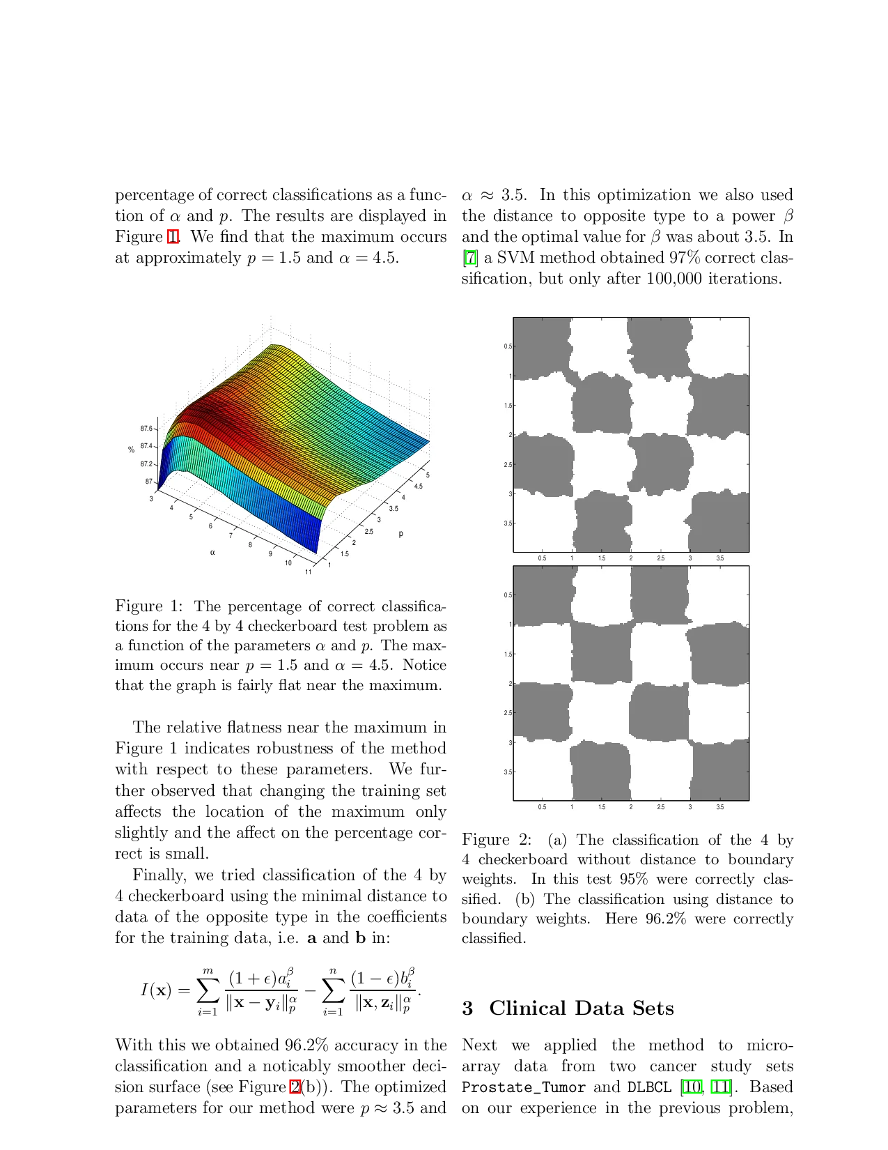
Rather than a i = b i = 1 we might consider other weightings of training points. We would want to make the choice of a = (a 1 , a 2 , . . . , a m ) and b = (b 1 , b 2 , . . . , b n ) based on easily available information. An obvious choice is the set of distances to other test points. In the checkerboard experiment below we demonstrate that training points too close to the boundary between Y and Z have undue influence and cause irregularity in the decision curve. We would like to give less weight to these points by using the distance from the points to the boundary. However, since the boundary is not known, we use the distance to the closest point in the other set as an approximation. We show that this approach gives improvement in classification and in the smoothness of the decision surface.
Note that if p = 2 in (2) our method limits onto the usual nearest neighbor method as α = β → ∞ since for large α the term with the smallest denominator will dominate the sum. For finite α our method gives greater weight to nearby points.
In the following we report on tests of the efficacy of the method using various ℓ p norms as the distance, various choices of α = β and a few simple choices for c, a, and b.
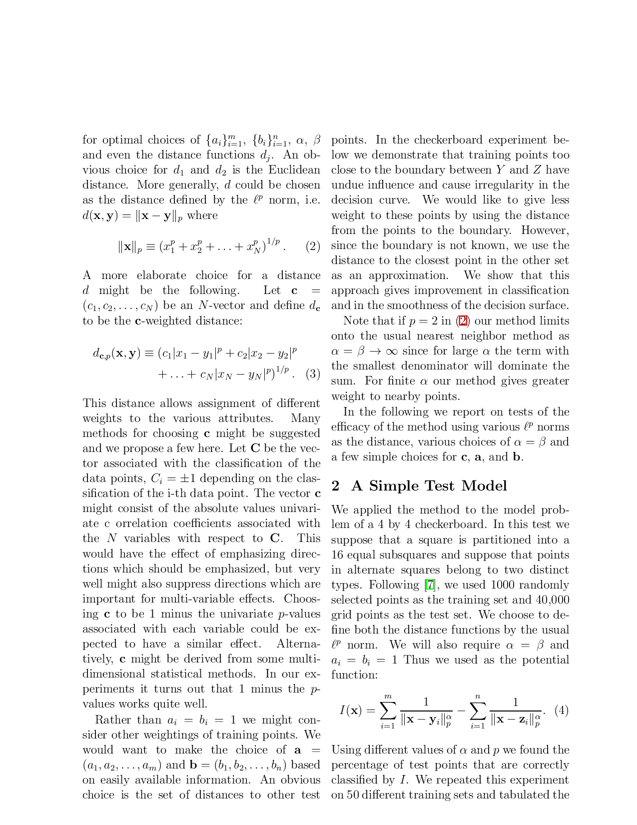
We applied the method to the model problem of a 4 by 4 checkerboard. In this test we suppose that a square
…(Full text truncated)…
This content is AI-processed based on ArXiv data.