Probabilistic reasoning with answer sets

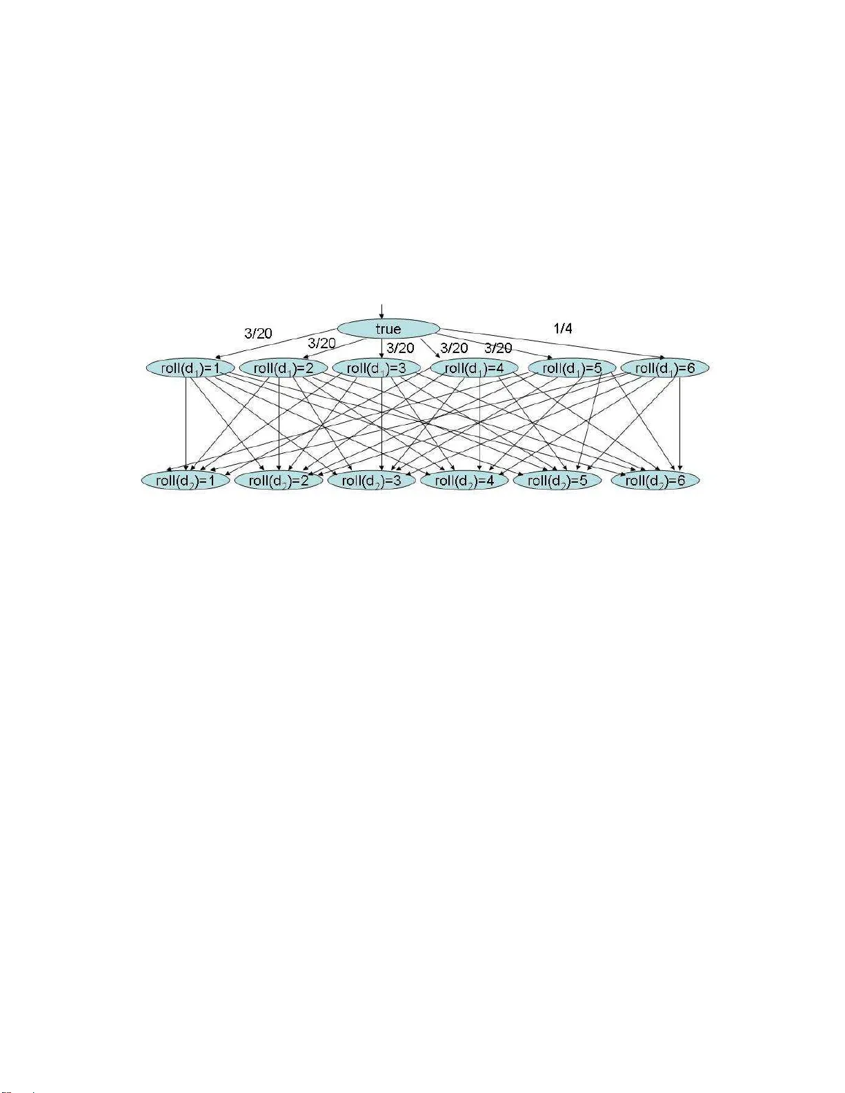
Under conside ratio n for public ation in Theory and Practice of Logic Pro grammi ng 1 Pr obabilistic r easoning with answer sets Chitta Baral † , Michael Gelfond ♯ , and Nelson Rushton ♯ † Department of Computer Science and Engineerin g, Arizona State Univer sity , T empe , AZ 85287-8809, USA. chi tta@asu.edu ♯ Department of Computer Scie nce T ex as T ec h Universit y Lubboc k, T exas 79409 { mgel fond,nrushton } @cs.ttu.edu submitte d 22 Sept ember 2005; re vised 21 J une 2007, 20 J une 2008; acce pted 2 D ecembe r 2008 Abstract T o appear in Theory and Practice of Logic Programm ing (TPLP) This paper dev elops a declarativ e language, P-l og, that combines logical and probabilistic argum ents in i ts reasoning. Answer Set Prolog is used as t he logical foundation, while causal Bayes nets serve as a probabilistic foundation. W e giv e seve ral non- trivial examples and illustrate the use of P-log for knowled ge representation and updating of kno wledge. W e argue that our approach to updates is more appealing than existing approaches. W e giv e sufﬁcienc y conditions for the coherency of P-log programs and sho w that Bayes nets can be easily mapped to coherent P-log programs. KEYWORDS : Logic prog ramming, answer sets, probabilistic reasoning, Answer Set Prolog 1 Introduction The goal of th is pap er is to deﬁne a knowledge representation language allowing natural, elaboratio n tolerant representatio n of common sense knowledge inv olving logic and probab ilities. The result of this effort is a language called P -log. By a kno wledge representation languag e, or KR lang uage, we mean a formal lang uage L with an enta ilment r elation E such that (1 ) statements of L capture the mean ing of some class of sentences of n atural langua ge, and (2) when a set S of natur al langua ge sentences is tr anslated into a set T ( S ) of statemen ts of L , the fo rmal consequ ences of T ( S ) u nder E are translations of the inform al, co mmonsen se con sequences of S . One of the best known KR languages is predicate calculus, and this example can be used to illustrate several points. First, a KR languag e is co mmitted to an entailment relation, b u t it is not comm itted to a particu lar infer ence algorithm . Research on infe rence mechanisms for pred icate calculus, for example, is still ongo ing while predicate calculus itself remains unchang ed since th e 1920’ s. Second, the m erit o f a KR languag e is p artly d etermined b y the class of statements rep resentable in it. Inf erence in predicate calcu lus, e.g., is very expensive, but it is an im portan t langu age be cause of its ab ility to for malize a broad class of natural language statements, arguably including m athematical discourse. Thoug h representatio n of mathematical discou rse is a p roblem solved to the satisf action of many , representation of 2 C. Baral, M. Gelfond and N . Rushton other kinds of discourse r emains an area of acti ve research, including w ork on defaults, modal re asoning, temp oral reasoning , an d varying d egrees of certainty . Answer Set Prolog (ASP) is a successfu l KR language with a large history of liter ature an d an acti ve commun ity o f researchers. In the last d ecade ASP was shown to be a powerful tool capable of represen ting recursiv e deﬁnitions, defaults, causal relations, special forms of self-reference, and other langua ge c onstructs which occur frequ ently in various no n-mathe matical d omains (Baral 200 3), an d are difﬁcult or impossible to express in classical logic and other commo n formalisms. ASP is based on the an swer set/stable mod els semantics (Gelfond et al. 1988) of lo gic progr ams with default ne gation (com monly written as not ), an d has its roots in research on non- mono tonic logics. In addition to th e default negation the language contains “classical” or “strong” negation (comm only wr itten as ¬ ) and “epistemic disjunction” (commo nly written as or ). Syntactically , an ASP program is a collection of rules of the form: l 0 or . . . or l k ← l k +1 , . . . , l m , not l m +1 , . . . , not l n where l ’ s ar e literals, i.e. expr essions o f the fo rm p and ¬ p where p is an a tom. A ru le with variables is viewed as a schem a - a sh orthand notation for th e set of its ground instan tiations. Infor mally , a gr ound prog ram Π can be viewed as a speciﬁcation for th e sets of beliefs whic h could be held by a rational reasoner associated with Π . Such sets are referred to as answer sets . An answer set is represented by a collection of ground literals. In for ming answer sets the reasoner must be guided by the following i nform al pr inciples: 1. One sh ould satisfy the r ules of Π . In other words, if on e believ es in the bo dy of a r ule, one mu st also be liev e in its head. 2. One should not believe in contrad ictions. 3. One should adhere to the rationality principle, which says: “Belie ve nothing you are not forced to belie ve. ” An an swer set S of a pr ogram satisﬁes a literal l if l ∈ S ; S satisﬁes not l if l 6∈ S ; S satisﬁes a d isjunction if it satisﬁes at least one of its members. W e often say that if p ∈ S then p is believed to b e true in S , if ¬ p ∈ S then p is believed t o b e false in S . Otherwise p is unknown in S . Consider , for in stance, an ASP p rogr am P 1 consisting of rules: 1. p ( a ) . 2. ¬ p ( b ) . 3. q ( c ) ← not p ( c ) , not ¬ p ( c ) . 4. ¬ q ( c ) ← p ( c ) . 5. ¬ q ( c ) ← ¬ p ( c ) . The ﬁrst two rules of th e program tell the age nt associated with P 1 that he mu st believe th at p ( a ) is true and p ( b ) is false. Th e third rule tells the agen t to belie ve q ( c ) if he believes neith er truth nor falsity of p ( c ) . Since the agent has r eason to believe neith er truth nor falsity of p ( c ) h e m ust b eliev e q ( c ) . Th e last two r ules r equire the agen t to in clude ¬ q ( c ) in an an swer set if this answer set con tains e ither p ( c ) or ¬ p ( c ) . Since the re is no reason for either of these con ditions to be satisﬁed, the p rogram will have uniq ue answer set S 0 = { p ( a ) , ¬ p ( b ) , q ( c ) } . A s expected the agent believes that p ( a ) and q ( c ) are true and that p ( b ) is false, an d simply does no t con sider tr uth or falsity of p ( c ) . If P 1 were expanded by another rule: 6. p ( c ) or ¬ p ( c ) Pr ob abilistic r easoning wi th answer sets 3 the ag ent will have two po ssible sets of beliefs re presented by answer sets S 1 = { p ( a ) , ¬ p ( b ) , p ( c ) , ¬ q ( c ) } and S 2 = { p ( a ) , ¬ p ( b ) , ¬ p ( c ) , ¬ q ( c ) } . Now p ( c ) is n ot ignor ed. In stead the agent consid ers two possible answer sets, one containin g p ( c ) an d another containing ¬ p ( c ) . Both, of co urse, contain ¬ q ( c ) . The example illustrates that the d isjunction (6), read as “belie ve p ( c ) to be tr ue or b elieve p ( c ) to b e false”, is certainly not a tautology . It is o ften called the awareness axiom (for p ( c ) ). T he axiom proh ibits the agent from removing truth of falsity of p ( c ) from consideratio n. Instead it forces h im to consider the con sequence s of believing p ( c ) to be true as well as the con sequences of belie ving it to be false. The above intuition ab out the meaning of logica l con nectives of ASP 1 and that of the ra tionality pr inciple is formalized in the deﬁnition of an answer set of a logic program (see Appendix I II). There is a substantial amount of literature on the methodo logy of using the languag e of ASP for representing various typ es of (p ossibly inco mplete) knowledge (Baral 2 003). There are by now a large number of inference engines designed for v arious subclasses of ASP programs. For example, a num ber of recently developed systems, called answer set solvers , ( Niemel ¨ a and Simons 1997; 20 02 ; Citrigno et al. 1997; Leone et al. 2006; Lierler 2005; Lin an d Zhao 2004; Gebser et al. 2007) compute answer sets of log ic pro grams with ﬁnite Herbr and un i verses. Answer set progr amming , a pr ogramm ing method ology which consists in red ucing a co mputatio nal problem to co mputing answer sets of a p rogram associated w ith it, has b een successfully applied to solu tions of various classical AI and CS task s including plannin g, diag nostics, and con- ﬁguration (Baral 2003). As a secon d example, mo re tr aditional query-a nswering algo rithms of log ic programm ing including SLDNF based Prolog inter preter an d its v ariants (Apt and Doets 1994; C hen, Swift and W arren 1995) are sound with respect to stable model semantics of programs without ¬ and or . Howe ver , ASP r ecognize s only th ree truth v alues: true, false, an d unknown. This paper discusses an augmen tation of ASP with constructs for represen ting varying degrees of b elief. The o bjective of the r esulting languag e is to allow elab oration tolerant repr esentation of common sense knowledge inv olving logic and probabilities. P-log was ﬁrst introdu ced in (Baral et al. 2004), but much of the mater ial here is n ew , as discussed in the co ncludin g sectio n of this paper . A prototype imp lementation o f P-log exists and has been used in p romising experiments comp aring its perfo rmance with existing appr oaches (Gelf ond et al. 2006). Howe ver, the f ocus o f this paper is not on algorithm s, but o n p recise declarative sem antics f or P-lo g, ba sic math ematical pr operties of the langu age, an d illustrations of its use. Such semantics are p rerequ isite for serious research in alg orithms related to th e language, because they gi ve a deﬁnition with respect to w hich co rrectness o f algor ithms can be judged. As a declarative langu age, P-log stands ready to borrow and co mbine existing an d future algorithms from ﬁelds such as answer set prog ramming , satisﬁability solvers, and Bayesian networks. P-log extends ASP by adding pr obabilistic constructs, where prob abilities are understoo d a s a measur e of the degree o f an ag ent’ s b elief. Th is extension is natu ral be cause the intuitive semantics of an ASP program is given in terms of the beliefs of a rational a gent associated with it. In additio n to the usual AS P statements, th e P-lo g progr ammer m ay declare “ran dom attributes” (essentially ran dom variables) of the form a ( X ) wh ere X and th e value o f a ( X ) range over ﬁnite d omains . Pro babilistic info rmation abo ut possible values of a is given throu gh causal probab ility ato ms , or pr - atoms. A pr -a tom takes rough ly th e form pr r ( a ( t ) = y | c B ) = v where a ( t ) is a rando m attribute, B a set of literals, an d v ∈ [0 , 1 ] . The statemen t says that if the value of a ( t ) is ﬁxed by e xperimen t r , and B holds, then the probab ility th at r causes a ( t ) = y is v . 1 It should be noted that the connec ti v es of Answer Set Prolog are diff erent from those of Propositional Logic. 4 C. Baral, M. Gelfond and N . Rushton A P-log prog ram co nsists o f i ts l ogical part an d its p robabilistic part. The logical part repr esents kn owledge which determines the possible worlds o f the pr ogram, includ ing ASP ru les and declaratio ns of rand om attributes, while the probabilistic part contains pr -atoms which determin e the probabilities of th ose worlds. If Π is a P-log p rogra m, the semantics o f P-log associates the logical part of Π with a “p ure” ASP p rogra m τ (Π) . The semantics of a g roun d Π is then given by (i) a collection of answer sets of τ (Π) v iewed as the possible sets of b eliefs of a ratio nal agent associated with Π , and (ii) a measure over the po ssible worlds d eﬁned by the collection of the proba bility a toms of Π and the principle of indifference which says that p ossible values o f r andom attribute a are assumed to b e equ ally p robab le if we h ave no reason to prefer one of them to any other . As a simple example, consider the program a : { 1 , 2 , 3 } . r andom ( a ) . pr ( a = 1 ) = 1 / 2 . This pr ogram deﬁnes a rando m attribute a with po ssible values 1 , 2 , an d 3 . The pro gram’ s possible w orlds are W 1 = { a = 1 } , W 2 = { a = 2 } , and W 3 = { a = 3 } . In accordance with the probability atom o f the pr ogram , the probab ility m easure µ ( W 1 ) = 1 / 2 . By the principle of indifference µ ( W 2 ) = µ ( W 3 ) = 1 / 4 . This paper is conce rned with deﬁning the syn tax and seman tics of P-log , and a meth odolo gy of its use fo r knowl- edge rep resentation. Whereas much of the curr ent research in p robabilistic lo gical langu ages focuses on lea rning, our m ain p urpose, by con trast, is to elegantly and straigh tforwardly rep resent kn owledge requirin g su btle logical and p robab ilistic reasonin g. A limitation of the cu rrent version of P- log is that we limit the discussion to models with ﬁnite Herbrand domains. This is common for ASP and its e xtensions. A related limitation prohibits pro- grams con taining inﬁnite n umber of random selections (and hence an uncountable number of possible world s). This mean s P-log cannot be u sed, fo r example, to d escribe stochastic pro cesses whose time domains are inﬁn ite. Howe ver , P-log can be used to describe in itial ﬁnite segments of such processes, and this paper gi ves two small ex- amples of s uch descriptions (Sections 5 .3 and 5 .4) and d iscusses one lar ge e xample in Sectio n 5.5. W e believe the technique s used by (Sato 19 95) can be used to extend the semantics of P-log to account for program s with in ﬁnite Herbrand do mains. Th e resultin g lang uage would, of c ourse, allow r epresentation o f pr ocesses with inﬁnite time domains. Even th ough such extension is the oretically n ot difﬁcult, its imp lementation requir es further research in ASP solvers. This matter is a subject of fu ture w ork. In th is paper we do not emphasize P-lo g inference algo rithms ev en for pr ograms with ﬁnite Herbrand domains, tho ugh this is a lso an obvious top ic for future work . Howe ver , our prototy pe im plementation of P-log, based on an a nswer set solver Smodels (Niemel ¨ a and Simo ns 1997), already works rather efﬁciently for pr ograms with large and co mplex lo gical comp onent and a comparativ ely small n umber of random attributes. The existing implementa tion of P-log was successfully used for instanc e in an ind ustrial size applica- tion fo r diagn osing faults in the reactiv e control system (RCS) of the space shuttle (Balduccini et al. 2001; Balduccini et al. 2002). Th e RCS is the Shuttle’ s system that has p rimary resp onsibility f or m aneuvering the air- craft while it is in spa ce. It consists of fuel and oxidizer tanks, valves, and other p lumbing needed to provide propellan t to the man euvering jets of the Shuttle. It also inclu des e lectronic circu itry: bo th to co ntrol th e valves in the fuel lin es and to pr epare th e jets to receive ﬁring c ommand s. Overall, th e system is rather co mplex, in th at it includ es 1 2 tanks, 4 4 jets, 66 valves, 33 switches, and aro und 160 com puter command s (co mputer-gener ated signals). W e believe that P- log h as so me distinctive fe atures w hich can be of in terest to those wh o use probab ilities. First, P-log pro babilities are deﬁned by th eir relatio n to a k nowledge base, repr esented in the f orm of a P-log progr am. Hence we give an account of the relationship between probabilistic models and the b ackgro und knowledge o n Pr ob abilistic r easoning wi th answer sets 5 which they are based. Sec ond, P-log gi ves a natural acc ount of ho w degrees o f belief c hange with the ad dition of new knowledge. For example, the standa rd deﬁnition of cond itional probability in our framework becomes a theorem , relatin g degrees of belief computed from tw o different knowledge b ases, in the special ca se where one knowledge base is obtained from th e o ther by the addition of obser vations whic h eliminate possible worlds. Moreover , P-lo g can accommodate u pdates which add rules to a knowledge b ase, including defaults and rules introdu cing new terms. Another importan t feature of P-log is its ability to distinguish between conditio ning on observations an d on delib- erate actions. The distinctio n was ﬁrst explicated in (Pearl 200 0), where, among other thing s, the author discusses relev ance of the distinction to a nswering q uestions about desirab ility of various actions (Simpson parad ox dis- cussed in section 5.2 gives a speciﬁc exam ple of such a situation) . In Pearl’ s approa ch the effect o f a deliberate action is modeled by an oper ation on a g raph representing causal r elations between random v ariables of a do main. In our appr oach, the semantics of co nditionin g on actions is ax iomatized u sing ASP’ s default n egation, and these axioms are included as par t o f th e translation of pr ograms from P-log to ASP . Because Pearl’ s theo ry of causal Bayesian n ets ( CBN’ s) ac ts as the prob abilistic fo undatio n of P-log , CBN’ s are deﬁned p recisely in Appen dix II, where it is shown th at each CBN maps in a natural way to a P-log program. The la st characteristic featu re o f P-log we would like to mention h ere is its probab ilistic no n-mon otonicity — that is, the ability o f the rea soner to chang e his probab ilistic m odel as a result of new information . No rmally any solution o f a probabilistic pro blem starts with constru ction of probabilistic m odel of a domain. The model consists of a co llection of po ssible worlds and the corr espondin g pro bability m easure, which togeth er determine the degrees of the reason er’ s b eliefs. In most appr oaches to pro bability , n ew infor mation can cau se a rea soner to abando n some of his po ssible worlds. Hen ce, the effect of up date is mo notonic, i.e. it can o nly elimina te possible worlds. Formalisms in which an update can cause creation of new po ssible worlds are called “probabilistically non-m onoton ic”. W e claim th at non -mono tonic p robabilistic systems such as P- log can nicely captu re chang es in the reasoner’ s pro babilistic models. T o clarify the argument let us inform ally consider the fo llowing P-log progr am (a more elaborate example involving a Moving Robot wil l be given in Section 5 .3). a : { 1 , 2 , 3 } . a = 1 ← not abnormal . r andom ( a ) ← abnormal . Here a is an attrib ute with po ssible v alues 1 , 2 , and 3 . The second rule of the progr am say s that n ormally the v alu e of a is 1 . The th ird rule tells us that under abnor mal circumstances a will rando mly take on o ne of its possible values. Since the progr am contains no atom abnormal th e second rule conclu des a = 1 . Th is is the o nly possible world of the prog ram, µ ( a = 1) = 1 , and hence th e value of a is 1 with probab ility 1 . Suppose, howe ver , that the p rogram is expan ded by an atom abnormal . This tim e the secon d r ule is no t app licable, and the pr ogram has three p ossible worlds: W 1 = { a = 1 } , W 2 = { a = 2 } , an d W 3 = { a = 3 } . By the p rinciple of ind ifference µ ( W 1 ) = µ ( W 2 ) = µ ( W 3 ) = 1 / 3 – attribute a takes on value 1 with probability 1 / 3 . The rest of the paper is organiz ed a s follows. In Section 2 we gi ve the s yntax of P-log and in Section 3 we give its semantics. In Section 4 we discuss updates o f P-log programs. Section 5 contains a n umber of examp les of the use of P-lo g fo r knowledge rep resentation and reasonin g. T he emp hasis here is on d emonstrating the power o f P-log and the metho dolog y of its use. In Sec tion 6 we p resent sufﬁciency condition s for consistency o f P-lo g p rogra ms and use it to show how Bayes nets are special cases of consistent P- log pr ograms. Section 7 c ontains a discussion of the relationsh ip between P-log and oth er langu ages combining probab ility and logic program ming. Section 8 d iscusses conclusions and future work . Ap pendix I contain s the proofs o f the major theorems, an d ap pendix II co ntains background material on causal B ayesian networks. Append ix III c ontains the deﬁnition and a short discussion of the notion of an answer set of a logic progr am. 6 C. Baral, M. Gelfond and N . Rushton 2 Syntax of P-log A probab ilistic logic program (P-log prog ram) Π consists of (i) a sorted signa ture , (ii) a declaration , (iii) a regular part , ( iv) a set of random selection ru les , ( v) a probab ilistic in formatio n part, and (vi) a set of observations and actions . Every statemen t of P-log must be ended by a period. (i) Sorted Signa ture : The sor ted signature Σ of Π co ntains a set O of objects an d a set F of f unction symbo ls. The set F is a un ion of two disjoin t sets, F r and F a . Elements o f F r are called term building functions . Elements of F a are called attributes . T erms of P-log are f ormed in a usual manner using function symbols from F r and objects from O . Expr essions o f the form a ( t ) , wh ere a is an attribute and t is a vector of term s of th e sorts requ ired by a , will be referr ed to a s attribute terms . (No te tha t attribute ter ms are n ot ter ms). Attributes with the rang e { tru e , false } are re ferred to as Boolean attrib utes or relations . W e assume that the number of terms and attributes ov er Σ is ﬁnite . Note that, since our sign ature is sorted , this does n ot p reclude th e use of func tion symb ols. The example in Section 5.5 illustra tes such a use. Atomic statements are o f the form a ( t ) = t 0 , wh ere t 0 is a term, t is a vector o f terms, and a is an attribute (w e assume th at t and t are o f th e sorts require d by a ). An atomic statem ent, p , or its negation, ¬ p is refe rred to as a literal (or Σ -literal, if Σ needs to be emphasized ); literals p and ¬ p are called contrary ; by l we den ote the literal contrary to l ; expressions l and not l wh ere l is a literal a nd not is the default negation of Answer Set Prolog are called extended literals . Literals of the fo rm a ( t ) = tru e , a ( t ) = false , an d ¬ ( a ( t ) = t 0 ) a re often written as a ( t ) , ¬ a ( t ) , and a ( t ) 6 = t 0 respectively . If p is a un ary relation and X is a variable then an e xpression of the form { X : p ( X ) } will be called a set-term . Occurrences of X in such an expression are referred to as bound . T erms an d literals are n ormally d enoted b y (possibly indexed) letters t an d l respecti vely . Th e letters c and a , possibly with in dices, are used as ge neric n ames for so rts and attributes. Other lower case letters deno te objects. Capital letters normally stand for variables. Similar to Answer Set Prolog, a P-log statement co ntaining unbo und variables is considered a shorthan d for the set of its ground in stances, where a g roun d instance is ob tained by replacin g unbou nd o ccurren ces of variables with pro perly so rted g round terms. Sorts in a progr am are indicated by the declaration s of attributes ( see below). In deﬁn ing semantics o f ou r langu age we limit our attention to ﬁnite p rogram s with no unbo und oc currenc es o f variables. W e sometimes refer to prog rams without unbound occurrences of v ariables as groun d . (ii) Declaration : The declaration of a P- log program is a collection of deﬁn itions of sorts and so rt declarations for attributes. A sort c can be deﬁned by explicitly listing its elements, c = { x 1 , . . . , x n } · (1) or by a logic progra m T with a uniqu e answer set A . In the latter c ase x ∈ c iff c ( x ) ∈ A . The domain and range of an attribute a are given by a statemen t of the form: a : c 1 × . . . × c n → c 0 · (2) For att ributes without parameters we simply write a : c 0 . The following examp le will be used throughou t this section. Example 1 Pr ob abilistic r easoning wi th answer sets 7 [Dice Example: progra m co mpon ent D 1 ] Consider a domain containing two dice owned by Mike and John r espectively . Each of th e d ice will be rolled on ce. A P-lo g prog ram Π 0 modeling th e dom ain will have a signatur e Σ co ntaining th e n ames of the two dice, d 1 and d 2 , an a ttribute ro l l mapping ea ch die to the value it ind icates when thr own, which is an in teger f rom 1 to 6 , an attribute owner mapping each die to a person , relation even ( D ) , where D rang es over dic e , and “imp orted” or “predeﬁne d” arithmetic fu nctions + and mo d . The cor respond ing dec larations, D 1 , will be as follows: dic e = { d 1 , d 2 }· sc or e = { 1 , 2 , 3 , 4 , 5 , 6 }· p erson = { mike , john }· r ol l : dic e → sc or e · owner : dic e → p erson · even : dic e → Bo ole an · ✷ (iii) Reg ular pa rt : The regular p art of a P-lo g p rogra m consists of a collection o f ru les of Answer Set Prolog (without disjunction) formed using literals of Σ . Example 2 [Dice Example (continu ed): pr ogram componen t D 2 ] For i nstance, the regular part D 2 of progr am Π 0 may contain the following ru les: owner ( d 1 ) = mike · owner ( d 2 ) = john · even ( D ) ← r ol l ( D ) = Y , Y mo d 2 = 0 · ¬ even ( D ) ← not even ( D ) · Here D and Y range over d ic e an d sc or e re spectiv ely . ✷ (iv) Random Selection : This sectio n contains rules describin g p ossible values of rand om attributes. More precisely a random selection is a rule of the form [ r ] r andom ( a ( t ) : { X : p ( X ) } ) ← B · (3) where r is a term u sed to n ame the ru le and B is a co llection of extend ed literals of Σ . T he n ame [ r ] is op tional and can be omitted if the progr am con tains exactly one ran dom selectio n for a ( t ) . Sometimes we re fer to r as an experiment . Statemen t (3) says that if B holds, the value of a ( t ) is selected at r andom from th e set { X : p ( X ) } ∩ r ange ( a ) by e xperiment r , u nless this value is ﬁxed b y a deliberate a ction . If B in (3) is empty we simply write [ r ] r andom ( a ( t ) : { X : p ( X ) } ) · (4) If { X : p ( X ) } is equal to the r ange ( a ) then rule (3) ma y be written as [ r ] r andom ( a ( t )) ← B · (5) Sometimes we re fer to th e attribute term a ( t ) as random and to { X : p ( X ) } ∩ r ange ( a ) as the dynamic range of a ( t ) via r ule r . W e also say that a literal a ( t ) = y occurs in the h ead of (3) for every y ∈ r ange ( a ) , an d that any groun d in stance of p ( X ) and literals occurrin g i n B occur in the body of (3). 8 C. Baral, M. Gelfond and N . Rushton Example 3 [Dice Example (continu ed)] The fact that v alues of attrib ute r ol l : dic e → sc or e are rando m is expressed by the statement [ r ( D ) ] r andom ( r ol l ( D )) . ✷ (v) Pr obabilistic Information: Information abo ut probabilities of random attrib utes takin g particular values is giv en by probab ility atoms (or simply pr-atoms ) which ha ve the form : pr r ( a ( t ) = y | c B ) = v · (6) where v ∈ [0 , 1] , B is a collections of extended literals, pr is a spe cial sym bol not belong ing to Σ , r is th e n ame of a random selection rule for a ( t ) , and pr r ( a ( t ) = y | c B ) = v says that if the value of a ( t ) is ﬁxed by e xperiment r , and B holds, then the pro bability tha t r causes a ( t ) = y is v . (Note th at here we use ‘cause’ in the sense that B is an immed iate o r pr oximate cause o f a ( t ) = y , as opposed to an indirec t cause.) If W is a possible world of a pr ogram co ntaining (6) an d W satisﬁes b oth B and the bod y of rule r , then we will refer to v as the causal probab ility of the atom a ( t ) = y in W . W e say that a literal a ( t ) = y occurs in the head of (6), and that literals occurrin g in B occur in the body of (6). If B is em pty we simply write pr r ( a ( t ) = y ) = v · (7) If the program contains exactly one rule generating v a lues of a ( t ) = y the index r may be omitted. Example 4 [Dice Example (continu ed): pr ogram componen t D 3 ] For instance, the dice do main may in clude D 3 consisting of th e random declar ation of r ol l ( D ) given in Example 3 and the following p robability atoms: pr ( r ol l ( D ) = Y | c owner ( D ) = john ) = 1 / 6 · pr ( r ol l ( D ) = 6 | c owner ( D ) = mike ) = 1 / 4 . pr ( r ol l ( D ) = Y | c Y 6 = 6 , owner ( D ) = m ike ) = 3 / 20 . The above prob ability atom s conve y that the die owned by Jo hn is fair , while th e die owned b y Mike is biased to roll 6 at a prob ability of · 25 . ✷ (vi) Observations and a ctions : Observations an d actions are statements of the respectiv e forms obs ( l ) · do ( a ( t ) = y )) · where l is a literal. Observations are used to record the outcome s of rando m ev ents, i.e., rand om attributes, an d attributes dependent o n them. The dice domain may , for instance, contain { obs ( r ol l ( d 1 ) = 4) } reco rding the outcome of rollin g die d 1 . The statemen t d o ( a ( t ) = y ) indic ates th at a ( t ) = y is made true as a result of a deliberate ( non-r andom ) action. F or instan ce, { do ( r ol l ( d 1 ) = 4 ) } m ay in dicate that d 1 was simply put o n th e tab le in the descr ibed p osition. Similarly , we may have obs ( even ( d 1 )) . Here, even thou gh even ( d 1 ) is n ot a rand om attribute, it is dep enden t on the r andom attribute r ol l ( d 1 ) . If B is a collection of literals obs ( B ) denotes th e set { obs ( l ) | l ∈ B } . Similarly fo r do . The p recise mean ing of do and obs is captur ed b y ax ioms (9 – 1 3) in th e next section and discussed in Exa mple 18, an d in conn ection with Simp son’ s Paradox in sectio n 5.2. More discussion of th e difference b etween actio ns and observations i n the context of probabilistic reasoning can be found in (Pearl 2000). Pr ob abilistic r easoning wi th answer sets 9 Note th at limiting observable fo rmulas to literals is not essential. It is ca used by the syntactic restrictio n o f An swer Set Prolog which pr ohibits th e u se of arb itrary f ormulas. Th e r estriction could be lifted if instead of Answer Set Prolog we were to consider, say , its dialect from ( Lifschitz et al. 1999). For the sake o f simplicity we decided to stay with the original deﬁnition of Answer Set Prolog. A P-log pr ogram Π c an be viewed as consisting of two p arts. The logical part , wh ich is f ormed by declar ations, regular rules, random selection s, actions and observations, d eﬁnes possible worlds of Π . The probab ilistic par t consisting of p robab ility atoms de ﬁnes a measure over the p ossible world s, and hen ce deﬁnes the proba bilities of formu las. (If n o pr obabilistic in formatio n o n the n umber of possible values of a rand om a ttribute is available we assume that all these v alues are equally probable) . 3 Semantics of P-log The seman tics of a gro und P-log pr ogram Π is given by a collectio n of the possible sets o f beliefs o f a ra tional agent associated with Π , toge ther with their prob abilities. W e refer to th ese sets as possible worlds of Π . W e will deﬁne the semantics in tw o stages. First we will deﬁne a mapping of the logical p art of Π into its Answer Set Prolog counterpart, τ (Π) . The answer sets of τ (Π) will play the role of possible worlds o f Π . Next we will use the probab ilistic par t of Π to deﬁne a measure over th e possible worlds, and the probabilities of formulas. 3.1 Deﬁning possible worlds: The logical part o f a P -log program Π is translated in to an Answer Set Prolog pro gram τ (Π) in the following way . 1. Sort declaration s: F or e very s ort declaration c = { x 1 , . . . , x n } o f Π , τ (Π) con tains c ( x 1 ) , . . . , c ( x n ) . For all sorts that are deﬁned using an Answer Set Prolog program T in Π , τ (Π) con tains T . 2. Regular part: In what follows (po ssibly indexed) variables Y are free variables. A rule contain ing these variables will be viewed as shorthand for a collection of its grou nd instances with respect to the appropriate typing. (a) For each rule r in the regular part of Π , τ (Π) contains the rule obtained by replacing each occurrence of an atom a ( t ) = y in r by a ( t , y ) . (b) For each attrib ute term a ( t ) , τ (Π) contains the rule: ¬ a ( t , Y 1 ) ← a ( t , Y 2 ) , Y 1 6 = Y 2 · (8) which guaran tees that in ea ch answer set a ( t ) ha s at most one v alue. 3. Random selections: (a) For an attrib ute a , we have the rule: intervene ( a ( t )) ← do ( a ( t , Y )) · (9) Intuitively , intervene ( a ( t )) means that the value of a ( t ) is ﬁxed by a deliberate action. Semantically , a ( t ) will not be consider ed random in possible w orlds which satisfy intervene ( a ( t )) . (b) Each random selection rule of the form [ r ] r andom ( a ( t ) : { Z : p ( Z ) } ) ← B · with r ange ( a ) = { y 1 , . . . , y k } is translated to the following rules in Answer Set Prolog 2 a ( t , y 1 ) or . . . or a ( t , y k ) ← B , not intervene ( a ( t )) · (10) 2 Our P -log imple mentati on uses an equiv alent rule 1 { a ( t , Z ) : c 0 ( Z ) : p ( Z ) } 1 ← B , not intervene ( a ( t )) from the input lan guage of Smodels. 10 C. Baral, M. Gelfond and N . Rushton If the dynamic range of a in the selection ru le is not equal to its static range, i.e. expression { Z : p ( Z ) } is not omitted, then we also add the rule ← a ( t , y ) , not p ( y ) , B , not intervene ( a ( t )) · (11) Rule (10) selects the value of a ( t ) fr om its rang e while ru le (1 1) ensur es th at the selected value satisﬁes p . 4. τ (Π) co ntains actions and observations o f Π . 5. For each Σ -literal l , τ (Π) contains the rule: ← obs ( l ) , not l · (12) 6. For each atom a ( t ) = y , τ (Π) contain s the rule: a ( t , y ) ← do ( a ( t , y )) · (13) The rule (12) guaran tees that no possible world o f the prog ram fails to satisfy observation l . The ru le (13) makes sure the atoms that are made true by the action are indeed true. This completes our deﬁnition of τ (Π) . Before we p roceed with some additio nal deﬁn itions le t us commen t on the difference b etween r ules 12 and 13. Since the P-lo g p rogra ms T ∪ obs ( l ) and T ∪ {← not l } hav e possible worlds which are identica l except for pos- sible occurrences of obs ( l ) , the new ob servation simply eliminates some of the po ssible w orlds of T . This reﬂects understan ding of observations in classical p robab ility theory . In con trast, due to the po ssible non-m onoto nicity of the r egular part o f T , po ssible worlds o f T ∪ do ( l ) can be substantially different from those of T (as o pposed to merely fewer i n number ); as we will illustrate in Section 5 .3. Deﬁnition 1 [Possible worlds] An answer set of τ (Π) is called a possible world of Π . ✷ The set of a ll possible worlds of Π will be den oted by Ω(Π) . When Π is clear fro m co ntext we will simply write Ω . Note that due to our restriction on the signature of P-log program s po ssible worlds of Π are alw ays ﬁnite. Example 5 [Dice example continued: P-log p rogra m T 1 ] Let T 1 be a P-log progra m con sisting of D 1 , D 2 and D 3 described in Examples 1, 2 , 3 and 4. The Answer Set Prolog counterp art τ ( T 1 ) of T 1 will consist of the following rules: dic e ( d 1 ) . dic e ( d 2 ) . sc or e (1) . sc or e (2) . sc or e (3) . sc or e (4) . sc or e (5) . sc or e (6) . p erson ( mike ) . p erson ( john ) . owner ( d 1 , mike ) . owner ( d 2 , john ) . even ( D ) ← r ol l ( D , Y ) , Y mo d 2 = 0 . ¬ even ( D ) ← not even ( D ) . intervene ( r ol l ( D )) ← do ( r ol l ( D , Y )) . r ol l ( D , 1) or . . . or r ol l ( D , 6) ← B , not int ervene ( r ol l ( D )) . ¬ r ol l ( D , Y 1 ) ← r ol l ( D , Y 2 ) , Y 1 6 = Y 2 . Pr ob abilistic r easoning wi th answer sets 11 ¬ owner ( D , P 1 ) ← owner ( D , P 2 ) , P 1 6 = P 2 . ¬ even ( D , B 1 ) ← even ( D , B 2 ) , B 1 6 = B 2 . ← obs ( r ol l ( D , Y )) , not r ol l ( D , Y ) . ← obs ( ¬ r ol l ( D , Y )) , not ¬ r ol l ( D , Y ) . r ol l ( D , Y )) ← do ( r ol l ( D , Y )) . The translation also contains similar obs and do axioms for other attributes wh ich have be en omitted here. The v ariables D , P , B ’ s, an d Y ’ s range over dic e , p erson , b o ole an , and sc or e r espectively . (In the inpu t lang uage of Lp arse used by Smodels(Nieme l ¨ a and Simon s 1997) and sev eral other answer set solving systems this typ ing can be expressed by t he statement # domain dic e ( D ) , p erson ( P ) , sc or e ( Y ) . Alternatively c ( X ) c an be ad ded to the bod y of ev ery rule containing variable X with doma in c . I n the rest o f the paper we will ignore these details and simply use Answer Set Prolog with the typed variables as n eeded.) It is easy to check that τ ( T 1 ) has 36 answer sets which are p ossible worlds of P-log prog ram T 1 . Each such w orld contains a possible outcome of the throws of the dice , e.g. r ol l ( d 1 , 6) , r ol l ( d 2 , 3) . ✷ 3.2 Assigning measures of probab ility: There are certain r easonablen ess c riteria which we would like ou r program s to satisfy . These are nor mally easy to check for P-log pr ogram s. Howe ver , the conditions are described using quantiﬁcation over possible worlds, and so cannot be axiomatized in Answer Set Prolog . W e w ill state them as meta-level co nditions, as follows (from this point forward we will limit our attention to programs satis fying these criteria): Condition 1 [Unique selection rule] If rules [ r 1 ] r andom ( a ( t ) : { Y : p 1 ( Y ) } ) ← B 1 · [ r 2 ] r andom ( a ( t ) : { Y : p 2 ( Y ) } ) ← B 2 · belong to Π then no possible world of Π satisﬁes both B 1 and B 2 . ✷ The above con dition follows from the intuitive read ing of random selection rules. In particular , there canno t be tw o different ran dom experiments each of which determines t he value of the same a ttribute. Condition 2 [Unique probability assignment] If Π contain s a random selection rule [ r ] r andom ( a ( t ) : { Y : p ( Y ) } ) ← B · along with two dif ferent probability atoms pr r ( a ( t ) | c B 1 ) = v 1 and pr r ( a ( t ) | c B 2 ) = v 2 · then no possible world of Π satisﬁes B , B 1 , and B 2 . ✷ 12 C. Baral, M. Gelfond and N . Rushton The justiﬁcation of Condition 2 is as f ollows: If the cond itions B 1 and B 2 can po ssibly b oth hold , an d we do n ot have v 1 = v 2 , then the in tuitiv e read ings of th e two pr -atoms are contrad ictory . On th e oth er h and if v 1 = v 2 , the same inf ormation is repr esented in multiple location s in the pr ogram which is bad for mainten ance and extension of the progra m. Note that we can st ill represent situations where the value of an attribute is determined by m ultiple possible c auses, as lo ng as the attribute is no t e xplicitly r andom. T o illustrate th is point let us consider a simple example fro m (V ennekens et al. 2006). Example 6 [Multiple Causes: Russian roulette with two guns] Consider a game of Ru ssian ro ulette with two six- chamber g uns. E ach o f the guns is loaded with a single bullet. What is the probab ility o f the player dying if he ﬁres both guns? Note th at in this example pulling the trigger of the ﬁrst gun and pu lling the trigg er o f the second gun are two indepen dent cau ses of the player’ s death . That is, the mechanisms of death from each of the two guns are separate and do not inﬂuence each other . The logical part of the story can be encoded by the following P-lo g progra m Π g : gun = { 1 , 2 } . pul l trigger : gun → b o ole an . % pul l trigger ( G ) says that the play er pulls the trigger of gun G . fatal : gun → b o ole an . % fatal ( G ) says that the bullet from gun G is sufﬁcient to kill the player . is de ad : b o ole an . % is de ad says that the player is de ad. [ r ( G )] : r andom ( fatal ( G )) ← pul l trigger ( G ) . is de ad ← fatal ( G ) . ¬ is de ad ← not is de ad . pul l trigger ( G ) . Here th e v alue of the ra ndom a ttribute fatal (1 ) , which stand s for “Gun 1 causes a wound s ufﬁcient to kill the player” is gener ated at rand om by ru le r (1) . Similarly fo r fatal (2) . Th e attribute is de ad , which stand s fo r the death of the player , is described in terms of f atal ( G ) an d hence is not explicitly random. T o deﬁne the prob ability of fatal ( G ) we will assume that when the cylind er of each gu n is spu n, each of the six chamb ers is equally likely to fall under the hammer . Thus, pr r (1) ( fatal (1)) = 1 / 6 . pr r (2) ( fatal (2)) = 1 / 6 . Intuitively the prob ability o f th e player’ s death will be 11 / 36 . At the end of this section we will learn how to compute this probability from the program. Suppose now that d ue to some mechanic al d efect the probability of the ﬁrst gun ﬁrin g its b ullet (and therefore killing the player) is not 1 / 6 but, say , 11 / 60 . Then the probability atoms above will be replace d by pr r (1) ( fatal (1)) = 1 1 / 60 . pr r (2) ( fatal (2)) = 1 / 6 . The pro bability of the play er’ s dea th deﬁned by the n ew progra m will be 0 · 32 . Obvio usly , both prog rams satisfy Conditions 1 and 2 above. Note howe ver that the somewhat similar program gun = { 1 , 2 } . pul l trigger : gun → b o ole an . is de ad : b o ole an . Pr ob abilistic r easoning wi th answer sets 13 [ r ( G )] : r andom ( is de ad ) ← pul l trigger ( G ) . pul l trigger ( G ) . does not satisﬁes Condition 1 and hence will not be allo wed in P-log. ✷ The next e xample presents a slightly different version of reasoning with multiple causes. Example 7 [Multiple Causes: The casino story] A r oulette wheel has 3 8 slots, two of which are gree n. Nor mally , the ball falls into one of these slots at random . Howe ver , th e game operator and the c asino o wner each ha ve buttons they can press which “rig” the wheel so that th e ball falls into slot 0 , which is gr een, with prob ability 1/2, wh ile the remaining slots ar e all eq ually likely . The game is rigged in the same way no matter which button is pressed, or if both are pr essed. I n this example, the rigg ing o f the game can b e viewed as having two causes. Supp ose in this particular game b oth buttons were pressed. What is the probability of the ball falling into slot 0 ? The story can be represented in P-log as follows: slot = { zer o , double zer o , 1 · · 36 } . button = { 1 , 2 } . pr esse d : button → b o ole an . rigge d : b o ole an . fal ls in : slot . [ r ] : r andom ( fal ls in ) . rigge d ← pr esse d ( B ) . ¬ rigge d ← not rigge d . pr esse d ( B ) . pr r ( fal ls in = zer o | c rigge d ) = 1 / 2 . Intuitively , the pro bability of th e b all falling into slot zero is 1 / 2 . The same result will be obtaine d by ou r form al semantics. N ote that the pr ogram obviou sly satisﬁes Cond itions 1 and 2. Howev er the following similar p rogra m violates Condition 2. slot = { zer o , double zer o , 1 · · 36 } . button = { 1 , 2 } . pr esse d : button → b o ole an . fal ls in : slot . [ r ] : r andom ( fal ls in ) . pr esse d ( B ) . pr r ( fal ls in = zer o | c pr esse d ( B )) = 1 / 2 . Condition 2 is violated here because two separ ate pr-atoms each assign pro bability to the literal fal ls in = zer o . Some oth er pro babilistic logic lang uages allow this, e mploying various systems of “combination rules” to compute the overall prob abilities of literals whose probability v alu es are multiply assigned. The study of combination rules is quite complex, and s o we av oid it here for simplicity . ✷ Condition 3 [No probabilities assigned outside of dynam ic ran ge] If Π contain s a random selection rule [ r ] r andom ( a ( t ) : { Y : p ( Y ) } ) ← B 1 · 14 C. Baral, M. Gelfond and N . Rushton along with probability atom pr r ( a ( t ) = y | c B 2 ) = v · then no possible world W o f Π satisﬁes B 1 and B 2 and not intervene ( a ( t )) but fails to satisfy p ( y ) . ✷ The cond ition ensur es that pr obabilities are only assign ed to lo gically possible o utcomes of ran dom selec tions. I t immediately follows fr om the intuitive reading of statements (3) and (6). T o better understan d the intu ition beh ind our deﬁnition of proba bilistic me asure it may be u seful to consider an intelligent a gent in th e pro cess of constru cting his possible worlds. Suppose he h as alre ady co nstructed a par t V of a (not yet complete ly con structed) possible world W , and su ppose that V satisﬁes the p recond ition o f some random selection rule r . Th e ag ent c an con tinue h is co nstruction by considerin g a rand om experime nt associated with r . If y is a po ssible outco me o f this experimen t then the agent may co ntinue his con struction by addin g th e atom a ( t ) = y to V . T o d eﬁne the pr obabilistic measure µ of the p ossible world W under co nstruction, we need to know the likelihood of y being the outcome of r , which we will call the causal probability of the atom a ( t ) = y in W . This info rmation can be obtained from a pr-atom pr r ( a ( t ) = y ) = v o f our p rogram or co mputed using the principle of ind ifference. In the latter case we need to consider the collection R of possible outcomes of experimen t r . For example if y ∈ R , there is no proba bility atom assignin g pro bability to o utcomes o f R , an d | R | = n , then the causal probability of a ( t = y ) in W will be 1 / n . Let v be the causal probab ility of a ( t ) = y . The atom a ( t ) = y may be dependent, in th e usual probabilistic sense, with other atom s already present in the c onstruction . Ho we ver v is not r ead as the p robability of a ( t ) = y , but the pro bability that, given what the agen t knows about the p ossible world at this po int in the con struction, the experiment determ ining the value of a ( t ) will have a certain r esult. Our assum ption is that these exper iments are indepen dent, a nd h ence it makes sen se tha t v will have a multiplicative effect on the p robability o f the possible world under construction . (This approach should be familiar to those accu stomed to working with Bayesian nets.) This intuition will be captured by the following deﬁn itions. Deﬁnition 2 [Possible outcomes] Let W be a consistent set of literals of Σ , Π be a P-log pro gram, a be an attribute, and y belon g to the range of a . W e say that the atom a ( t ) = y is possible in W with respect to Π if Π co ntains a rando m selection rule r for a ( t ) , where if r is of the form (3) then p ( y ) ∈ W and W satis ﬁes B , and if r is of the form (5) then W satisﬁes B . W e also say th at y is a possible ou tcome of a ( t ) in W with r espect to Π via ru le r , an d that r is a generatin g rule for the atom a ( t ) = y . ✷ Recall that, based on ou r c onv ention, if the range of a is boolean then we can just say th at a ( t ) and ¬ a ( t ) are possible in W . (Note that by Condition 1, if W is a possible w orld of Π then each atom p ossible in W has exactly one generating rule.) Note that, as discussed above, there is some subtlety here becau se we are describing a ( t ) = y as possible, though not necessarily true, with respect to a particular set of literals and program Π . For every W ∈ Ω(Π) and e very atom a ( t ) = y po ssible in W we will deﬁne the co rrespon ding causal probability P ( W , a ( t ) = y ) . Whenever possible, the p robab ility of an atom a ( t ) = y will be directly assign ed b y p r-atoms of the pro gram and den oted by P A ( W , a ( t ) = y ) . T o deﬁne pro babilities of the r emaining atoms we assum e that by default, all v alues o f a given attribute wh ich are not assigned a pro bability ar e eq ually lik ely . Their p robab ilities will be denoted by PD ( W , a ( t ) = y ) . ( P A stands for assigned probability and PD stands for default p robab ility ). For each atom a ( t ) = y possible in W : 1. Assigned prob ability: Pr ob abilistic r easoning wi th answer sets 15 If Π c ontains pr r ( a ( t ) = y | c B ) = v where r is th e generating rule of a ( t ) = y , B ⊆ W , and W does no t contain intervene ( a ( t )) , the n P A ( W , a ( t ) = y ) = v 2. Default probability : For any set S , let | S | deno te the cardina lity of S . Let A a ( t ) ( W ) = { y | P A ( W , a ( t ) = y ) is d eﬁned } , and a ( t ) = y be possible in W such that y 6∈ A a ( t ) ( W ) . Th en let α a ( t ) ( W ) = X y ∈ A a ( t ) ( W ) P A ( W , a ( t ) = y ) β a ( t ) ( W ) = |{ y : a ( t ) = y is possible in W a nd y 6∈ A a ( t ) ( W ) }| PD ( W , a ( t ) = y ) = 1 − α a ( t ) ( W ) β a ( t ) ( W ) 3. Finally , the causal prob ability P ( W , a ( t ) = y ) of a ( t ) = y in W is deﬁned by: P ( W , a ( t ) = y ) = ( P A ( W , a ( t ) = y ) if y ∈ A a ( t ) ( W ) PD ( W , a ( t ) = y ) oth erwise · Example 8 [Dice example continued: P-log p rogra m T 1 ] Recall the P-log program T 1 from Example 5. The progr am c ontains the following p robabilistic informatio n: pr ( r ol l ( d 1 ) = i | c owner ( d 1 ) = mike ) = 3 / 20 , for each i such that 1 ≤ i ≤ 5 · pr ( r ol l ( d 1 ) = 6 | c owner ( d 1 ) = mike ) = 1 / 4 · pr ( r ol l ( d 2 ) = i | c owner ( d 2 ) = john ) = 1 / 6 , for each i such that 1 ≤ i ≤ 6 · W e n ow consider a po ssible world W = { owner ( d 1 , mike ) , owner ( d 2 , john ) , r ol l ( d 1 , 6) , r ol l ( d 2 , 3) , . . . } of T 1 and compu te P ( W , r ol l ( d i ) = j ) fo r e very d ie d i and every po ssible score j . According to the above deﬁnition , P A ( W , ro l l ( d i ) = j ) and P ( W , ro l l ( d i ) = j ) are deﬁned f or every rand om atom (i.e. atom formed by a random attribute) r ol l ( d i ) = j in W as follows: P ( W , r ol l ( d 1 ) = i ) = P A ( W , r ol l ( d 1 ) = i ) = 3 / 2 0 , for each i such that 1 ≤ i ≤ 5 · P ( W , r ol l ( d 1 ) = 6 ) = P A ( W , r ol l ( d 1 ) = 6 ) = 1 / 4 · P ( W , r ol l ( d 2 ) = i ) = P A ( W , r ol l ( d 2 ) = i ) = 1 / 6 , for each i such that 1 ≤ i ≤ 6 · ✷ Example 9 [Dice example continued: P-log p rogra m T 1 · 1 ] In the pre vious example all rand om atoms o f W were assigne d pro babilities. Let u s now consider what will happen if explicit prob abilistic in formatio n is omitted. Let D 3 · 1 be ob tained from D 3 by rem oving all probab ility atom s except pr ( r ol l ( D ) = 6 | c owner ( D ) = mike ) = 1 / 4 . Let T 1 · 1 be the P-log pr ogram consisting o f D 1 , D 2 and D 3 · 1 and let W be as in the previous example. Only the atom r ol l ( d 1 ) = 6 will be giv en an assigned probability: P ( W , r ol l ( d 1 ) = 6 ) = P A ( W , r ol l ( d 1 ) = 6 ) = 1 / 4 . 16 C. Baral, M. Gelfond and N . Rushton The remaining atoms receiv e the e xpected default probabilities: P ( W , r ol l ( d 1 ) = i ) = PD ( W , r ol l ( d 1 ) = i ) = 3 / 2 0 , for each i such that 1 ≤ i ≤ 5 · P ( W , r ol l ( d 2 ) = i ) = PD ( W , r ol l ( d 2 ) = i ) = 1 / 6 , for each i such that 1 ≤ i ≤ 6 · ✷ Now we are read y to deﬁne the measure, µ Π , induce d b y the P-log progr am Π . Deﬁnition 3 [Measure] 1. Let W b e a p ossible world o f Π . T he unnor malized pro bability , ˆ µ Π ( W ) , of a possible world W induced by Π is ˆ µ Π ( W ) = Y a ( t , y ) ∈ W P ( W , a ( t ) = y ) where the produ ct is taken over atoms for which P ( W , a ( t ) = y ) is deﬁn ed. 2. Suppose Π is a P-log prog ram having at least on e p ossible world with no nzero un norma lized proba bility . The measure , µ Π ( W ) , o f a possible world W induced by Π is the u nnor malized probability of W divided by the sum of the unnorm alized probabilities of all p ossible worlds of Π , i.e., µ Π ( W ) = ˆ µ Π ( W ) P W i ∈ Ω ˆ µ Π ( W i ) When the program Π is clear from the context we may simply write ˆ µ and µ instead of ˆ µ Π and µ Π respectively . ✷ The unnormalize d measure of a p ossible world W corresp onds, f rom the st andpo int o f classical probability , to the uncon ditional pro bability o f W . Each random atom a ( t ) = y in W is thoug ht of as the ou tcome of a r andom experiment th at takes p lace in the construc tion of W , and P ( W , a ( t ) = y ) is the p robab ility of that experiment having the result a ( t ) = y in W . The multiplication in the deﬁnition o f un normalized m easure is justiﬁed by an assumption that all experimen ts p erform ed in the co nstruction of W are inde penden t. Th is is sub tle becau se the experiments themselves do not show up in W — only their results do, and the results may not be independ ent. 3 Example 10 [Dice example continued: T 1 and T 1 · 1 ] The measures of the possible worlds of Example 9 are gi ven by µ ( { r ol l ( d 1 , 6) , r ol l ( d 2 , y ) , . . . } ) = 1 / 2 4 , for 1 ≤ y ≤ 6 , and µ ( { r ol l ( d 1 , u ) , r ol l ( d 2 , y ) , . . . } ) = 1 / 4 0 , for 1 ≤ u ≤ 5 an d 1 ≤ y ≤ 6 . where only random atoms of each possible world are sho wn. ✷ Now we are read y for our main deﬁnition. 3 For i nstance , in the upc oming Example 18, random attri but es arsenic and de ath respecti vely reﬂect wheth er or not a gi ven rat ea ts arsenic, and whethe r or not it dies. I n that e xample, de ath and arsenic are clea rly dependent. Howe ver , we assume that the f acto rs which determine whether a poisoning will lead to death (such as the rat’ s constitu tion, and the strength of the poison) are indepe ndent of the fac tors which determin e whether poisoni ng occurred in the ﬁrst place. Pr ob abilistic r easoning wi th answer sets 17 Deﬁnition 4 [Probab ility] Suppose Π is a P-log progra m having at lea st one p ossible w orld with nonzero u nnorm alized pro bability . The probab ility , P Π ( E ) , of a set E of po ssible worlds of program Π is the sum of the m easures of the possible worlds from E , i.e. P Π ( E ) = X W ∈ E µ Π ( W ) · ✷ When Π is clear from the context we may simply write P instead o f P Π . The fun ction P Π is n ot always de ﬁned, since n ot every syntactically c orrect P-lo g pro gram satisﬁes the co ndition of h aving at least one possible world with nonzero unnormalized measure. Consider f or instance a prog ram Π consisting of facts p ( a ) · ¬ p ( a ) · The pro gram has no answer sets at all, and henc e here P Π is n ot d eﬁned. The follo wing propo sition, howe ver , says that when P Π is deﬁned, it satisﬁes th e Kolmogorov axioms of pro bability . This justiﬁes o ur use of the term “proba bility” for the fu nction P Π . The prop osition follo ws stra ightforwardly from the deﬁnition. Pr op osition 1 [K olmogor ov Axioms] For a P-log program Π for which the function P Π is deﬁned we have 1. For any set E of po ssible worlds of Π , P Π ( E ) ≥ 0 . 2. If Ω is the set of all po ssible worlds of Π then P Π (Ω) = 1 . 3. For any d isjoint subsets E 1 and E 2 of possible worlds of Π , P Π ( E 1 ∪ E 2 ) = P Π ( E 1 ) + P Π ( E 2 ) . ✷ In logic-based prob ability theory a set E o f possible worlds is often represented by a pr oposition al formula F such that W ∈ E iff W i s a model of F . In this case the probab ility f unction may be deﬁned on proposition s as P ( F ) = def P ( { W : W is a model of F } ) . The value of P ( F ) is interp reted as the d egree of reasone r’ s belief in F . A similar id ea ca n be u sed in o ur frame- work. But since the con nectives of A nswer Set Pr olog are different fro m tho se of Prop ositional Log ic the notion of propositional formu la will be re placed by that of f ormula of Answer Set Pro log (ASP form ula). In this paper we limit our discussion to relativ ely simple class of ASP formulas which is suf ﬁcient for our purpose. Deﬁnition 5 [ASP Formulas (syntax)] For an y signature Σ • An extended literal of Σ is an ASP formu la . • if A and B are ASP formu las then ( A ∧ B ) and ( A or B ) are ASP form ulas. ✷ For example, (( p ∧ not q ∧ ¬ r ) or ( not r )) is an A SP for mula but ( not ( not p )) is no t. More gen eral deﬁnition of ASP formulas wh ich a llows the use of negations ¬ and not in front of arbitrary formu las can be fou nd in (Lifschitz et al. 2001). Now we deﬁn e the truth ( W ⊢ A ) and falsity ( W ⊣ A ) of an ASP fo rmula A with respect to a possible world W : 18 C. Baral, M. Gelfond and N . Rushton Deﬁnition 6 [ASP Formulas (semantics)] 1. For any Σ -liter al l , W ⊢ l if l ∈ W ; W ⊣ l if l ∈ W . 2. For any extend ed Σ -literal not l , W ⊢ not l if l 6∈ W ; W ⊣ not l if l ∈ W . 3. W ⊢ ( A 1 ∧ A 2 ) if W ⊢ A 1 and W ⊢ A 2 ; W ⊣ ( A 1 ∧ A 2 ) if W ⊣ A 1 or W ⊣ A 2 . 4. W ⊢ ( A 1 or A 2 ) if W ⊢ A 1 or W ⊢ A 2 ; W ⊣ ( A 1 or A 2 ) if W ⊣ A 1 and W ⊣ A 2 . ✷ An ASP formu la A wh ich is neither true nor false in W is undeﬁne d in W . Th is introdu ces so me subtlety . Th e axioms of modern mathem atical probability are viewed as axioms about measures on sets of possible worlds, and as such are satisﬁed b y P-log p robab ility measur es. However , since we are u sing a th ree-valued logic, some classical conseq uences of the ax ioms for the pro babilities of formu lae fail to hold . Thus, all theorem s of classical probab ility theor y can be applied in the context of P-log; b ut we must be careful how we interpr et set oper ations in terms of formulae. For example, no te that formula ( l or not l ) is true in every possible world W . Ho we ver fo rmula ( p or ¬ p ) is unde ﬁned in an y possible w orld containing neither p n or ¬ p . Thu s if P is a P-log probability measure, we will alw ays have P ( not l ) = 1 − P ( l ) , but not necessarily P ( ¬ l ) = 1 − P ( l ) . Consider for in stance an ASP p rogram P 1 from th e introd uction. If we expand P 1 by the a pprop riate declarations we obtain a p rogram Π 1 of P-log. It’ s only po ssible w orld is W 0 = { p ( a ) , ¬ p ( b ) , q ( c ) } . Since neither p nor q are random , its mea sure, µ ( W 0 ) is 1 ( since th e em pty pro duct is 1 ). Howe ver , since the truth value of p ( c ) or ¬ p ( c ) in W 0 is u ndeﬁned , P Π 1 ( p ( c ) or ¬ p ( c )) = 0 . This is n ot surpr ising since W 0 represents a po ssible set o f beliefs of the agent associated with Π 1 in which p ( c ) is simply ignored . (Note that the probability of formula q ( c ) which expresses this f act is properly equal to 1 ). Let u s n ow look a t p rogram Π 2 obtained f rom Π 1 by declarin g p to be a rando m attribute. Th is time p ( c ) is n ot ignored . I nstead the agent considers two possibilities and constructs tw o complete 4 possible worlds: W 1 = { p ( a ) , ¬ p ( b ) , p ( c ) , ¬ q ( c ) } and W 2 = { p ( a ) , ¬ p ( b ) , ¬ p ( c ) , ¬ q ( c ) } . Obviously P Π 2 ( p ( c ) or ¬ p ( c )) = 1 . It is easy to ch eck that if all po ssible worlds of a P-log progr am Π are comp lete then P Π ( l or ¬ l ) = 1 . This is the case for in stance when Π co ntains no re gular part, o r when the regular part of Π co nsists of d eﬁnitions of relations p 1 , . . . , p n (where a d eﬁnition of a relation p is a collection o f ru les which d etermines the truth value of a toms built from p to be true or false in all possible worlds). Now th e deﬁnition of probab ility can be expan ded to AS P formu las. Deﬁnition 7 [Probab ility of Formu las] The probab ility with resp ect to program Π of a f ormula A , P Π ( A ) , is the sum of the measures of the possible worlds of Π in which A is true, i.e. P Π ( A ) = X W ⊢ A µ Π ( W ) · ✷ As usual when con venient we omit Π a nd simply write P instead of P Π . 4 A possible world W of program Π is called complete if for any ground atom a from the signature of Π , a ∈ W or ¬ a ∈ W . Pr ob abilistic r easoning wi th answer sets 19 Example 11 [Dice example continued] Let T 1 be the p rogram fr om Exam ple 5. Th en, using the m easures comp uted in E xample 1 0 an d the deﬁn ition of probab ility we have, say P T 1 ( r ol l ( d 1 ) = 6 ) = 6 ∗ (1 / 2 4) = 1 / 4 . P T 1 ( r ol l ( d 1 ) = 6 ∧ even ( d 2 )) = 3 ∗ (1 / 24) = 1 / 8 . ✷ Example 12 [Causal probability equal to 1 ] Consider the P-log program Π 0 consisting of: a : b o ole an . r andom a . pr ( a ) = 1 · The translation of its logical part, τ (Π 0 ) , will consist of the following: intervene ( a ) ← do ( a ) . intervene ( a ) ← do ( ¬ a ) . a or ¬ a ← not int ervene ( a ) . ← obs ( a ) , n ot a . ← obs ( ¬ a ) , not ¬ a . a ← do ( a ) . ¬ a ← do ( ¬ a ) . τ (Π 0 ) h as two a nswer sets W 1 = { a , . . . } and W 2 = {¬ a , . . . } . Th e prob abilistic part of Π 0 will lead to the following pr obability assignments. P ( W 1 , a ) = 1 . P ( W 1 , ¬ a ) = 0 . P ( W 2 , a ) = 1 . P ( W 2 , ¬ a ) = 0 . ˆ µ Π 0 ( W 1 ) = 1 . ˆ µ Π 0 ( W 2 ) = 0 . µ Π 0 ( W 1 ) = 1 . µ Π 0 ( W 2 ) = 0 . This giv es us P Π 0 ( a ) = 1 . ✷ Example 13 [Guns example continued] Let Π g be the P-lo g progr am fr om Ex ample 6. It is not difﬁcult to c heck that the progr am has fo ur p ossi- ble worlds. All fo ur co ntain { gun (1) , gun (2 ) , pul l trigger (1) , pul l trigger (2 ) } . Sup pose now that W 1 contains { fatal (1) , ¬ fatal (2) } , W 2 contains {¬ fatal (1) , fatal (2) } , W 3 contains { fatal (1) , fatal (2) } , a nd W 4 contains {¬ fatal (1 ) , ¬ fatal (2) } . Th e ﬁrst three worlds contain is de ad , the last on e contains ¬ is de ad . Th en 20 C. Baral, M. Gelfond and N . Rushton µ Π g ( W 1 ) = 1 / 6 ∗ 5 / 6 = 5 / 36 . µ Π g ( W 2 ) = 5 / 6 ∗ 1 / 6 = 5 / 36 . µ Π g ( W 3 ) = 1 / 6 ∗ 1 / 6 = 1 / 36 . µ Π g ( W 4 ) = 5 / 6 ∗ 5 / 6 = 25 / 36 . and hence P Π g ( is de ad ) = 11 / 3 6 . ✷ As expe cted, this is exactly the intuiti ve answer from Ex ample 6. A similar argument ca n be used to compute probab ility o f rigge d from Example 7. Even if P Π satisﬁes the Kolmogorov axioms it may still co ntain questiona ble probab ilistic informa tion. For in- stance a pro gram containing statements pr ( p ) = 1 and pr ( ¬ p ) = 1 does not seem to have a clear intuitive meaning. The next deﬁnition is m eant to captur e the class of progr ams wh ich are logically and p robabilistically coheren t. Deﬁnition 8 [Program Coherency] Let Π be a P-log pro gram and Π ′ be ob tained from Π by removing all o bservations and actions. Π is said to be consistent if Π has at least on e possible world. W e will say tha t a consistent program Π is coheren t if • P Π is deﬁned . • For ev ery selection rule r with the prem ise K a nd every probability atom pr r ( a ( t ) = y | c B ) = v of Π , if P Π ′ ( B ∪ K ) is no t equal to 0 then P Π ′ ∪ obs ( B ) ∪ obs ( K ) ( a ( t ) = y ) = v . ✷ Coherency in tuitiv ely says that cau sal pr obabilities entail corr espondin g conditio nal probab ilities. W e now giv e two e xamples of program s who se probability functions are deﬁned, b ut which are not coheren t. Example 14 Consider the programs Π 5 : a : b o ole an . r andom a . a · pr ( a ) = 1 / 2 · and Π 6 : a : { 0 , 1 , 2 } . r andom a . pr ( a = 0 ) = pr ( a = 1) = pr ( a = 2) = 1 / 2 · Neither pr ogram is coh erent. Π 5 has one p ossible world W = { a } . W e have ˆ µ Π 5 ( W ) = 1 / 2 , µ Π 5 ( W ) = 1 , an d P Π 5 ( a ) = 1 . Since pr ( a ) = 1 / 2 , Π 5 violates condition (2) of coherency . Π 6 has three possible worlds, { a = 0 } , { a = 1 } , and { a = 2 } each with unno rmalized p robability 1 / 2 . Hence P Π 6 ( a = 0) = 1 / 3 , which is different fr om pr ( a = 0) which is 1 / 2 ; thus making Π 6 incohere nt. ✷ The following two p roposition s give conditions o n th e pr obability atoms of a P-log pro gram wh ich are necessary for its coherency . Pr ob abilistic r easoning wi th answer sets 21 Pr op osition 2 Let Π be a coh erent P- log progr am without any observations o r actions, and a ( t ) b e an attribute term from the signature of Π . Suppose that Π contain s a selection rule [ r ] r andom ( a ( t ) : { X : p ( X ) } ) ← B 1 · and ther e is a subset c = { y 1 , . . . , y n } of the rang e of a ( t ) such that fo r every possible world W of Π satisfying B 1 , we h av e { Y : W ⊢ p ( Y ) } = { y 1 , . . . , y n } . Supp ose a lso that f or some ﬁxed B 2 , Π contains pro bability atoms of the form pr r ( a ( t ) = y i | c B 2 ) = p i · for all 1 ≤ i ≤ n . Then P Π ( B 1 ∧ B 2 ) = 0 or n X i =1 p i = 1 ✷ Proof : Let ˆ Π = Π ∪ obs ( B 1 ) ∪ obs ( B 2 ) and let P Π ( B 1 ∧ B 2 ) 6 = 0 . Fr om this, to gether with rule 12 from th e deﬁnition of the mapp ing τ fr om section 3.1, we h av e that ˆ Π h as a possible world with non-zero pro bability . Henc e by Prop osition 1, P ˆ Π satisﬁes the K olmogo rov Axioms. By Condition 2 o f coher ency , we have P ˆ Π ( a ( t ) = y i ) = p i , for all 1 ≤ i ≤ n . By rule 1 2 of the deﬁnition of τ we have that e very possible world of ˆ Π satisﬁes B 1 . This, tog ether with rules 8, 10, and 11 from the sam e deﬁnitio n implies that ev ery possible world of ˆ Π con tains exactly one literal of the for m a ( t ) = y where y ∈ c . Since P ˆ Π satisﬁes the Kolmogorov axioms we have that if { F 1 , . . . , F n } is a set of literals exactly one of which is true in e very possible w orld of ˆ Π then n X i =1 P ˆ Π ( F i ) = 1 This implies that n X i =1 p i = n X i =1 P ˆ Π ( a ( t ) = y i ) = 1 The proof of the following is similar : Pr op osition 3 Let Π be a coh erent P- log progr am without any observations o r actions, and a ( t ) be an attribute term from the signature of Π . Suppose that Π contain s a selection rule [ r ] r andom ( a ( t ) : p ) ← B 1 · and ther e is a subset c = { y 1 , . . . , y n } of the rang e of a ( t ) such that fo r every possible world W of Π satisfying B 1 , we h av e { Y : W ⊢ p ( Y ) } = { y 1 , . . . , y n } . Supp ose a lso that f or some ﬁxed B 2 , Π contains pro bability atoms of the form pr r ( a ( t ) = y i | c B 2 ) = p i · for some 1 ≤ i ≤ n . Then P Π ( B 1 ∧ B 2 ) = 0 or n X i =1 p i ≤ 1 ✷ 22 C. Baral, M. Gelfond and N . Rushton 4 Belief Update in P-log In this section we ad dress the pr oblem of belief upd ating — th e ability of an agent to change degrees of b elief deﬁned by his current k nowledge ba se. If T is a P-log pro gram and U is a collection of statem ents such that T ∪ U is coheren t we call U an update of T . Intuitiv ely U is viewed as new inf ormation which can be added to an existent knowledge base, T . Ex plicit representa tion o f the ag ent’ s beliefs allows for a na tural trea tment of b elief update s in P-log. The r easoner should simply add the new knowledge U to T and check th at the result is co herent. If it is then the new degrees of the r easoner’ s b eliefs are given by th e func tion P T ∪ U . As men tioned bef ore we plan to expand our work on P-log with allo wing its regular pa rt be a program in CR -Prolog (Baldu ccini and Gelfond 2003) which has a much more liberal notio n of consistency than Answer Set Prolog. The resulting languag e will allow a substantially larger s et of possible upda tes. In what follo ws we compare an d contrast dif ferent types of up dates and in vestigate their relationship with the updating mechanisms of more traditional Bayesian approa ches. 4.1 P-log Updates and Conditional Probability In B ayesian probability theory the no tion of conditional pro bability is used as the p rimary mechanism for updating beliefs in ligh t of new inf ormation . I f P is a pro bability measure (in duced by a P-log pr ogram or other wise), then the co nditiona l proba bility P ( A | B ) is deﬁned a s P ( A ∧ B ) / P ( B ) , pr ovided P ( B ) is not 0 . In tuitively , P ( A | B ) is understood a s the probability of a formu la A with respect to a background theo ry and a set B of all of the agent’ s additio nal observations of the world. The new e v idence B simp ly eliminates the possible worlds which do not satisfy B . T o em ulate this type o f reason ing in P-log we ﬁrst assum e that the only fo rmulas ob servable by the agent ar e literals. (Th e restriction is need ed to stay in th e sy ntactic bo undar ies of our langua ge. As mentioned in Section 2 th is restrictio n is no t essential and can be eliminated by using a syntactically richer versio n of Answer Set Prolog.) Th e next theorem gives a relationship between classical cond itional proba bility and updates in P-lo g. Recall that if B is a set of literals, add ing the o bservation obs ( B ) to a pro gram Π has the effect of rem oving all possible worlds of Π which fail to satisfy B . Pr op osition 4 [Condition al Pro bability in P-log] For an y coherent P-log program T , fo rmula A , and a set of Σ -literals B suc h that P T ( B ) 6 = 0 , P T ∪ obs ( B ) ( A ) = P T ( A ∧ B ) / P T ( B ) In other words, P T ( A | B ) = P T ∪ obs ( B ) ( A ) ✷ Proof: Let us order all possible worlds of T in such a way that { w 1 · · · w j } is the set of all p ossible worlds of T that contain both A and B , { w 1 · · · w l } is the set of all possible worlds of T that co ntain B , and { w 1 · · · w n } is the set of all p ossible w orlds of T . Programs of Answer Set Prolog are monotonic with r espect to constraints, i.e. for any pr ogram Π and a set o f constraints C , X is an answer set of Π ∪ C iff it is an answer set of P satisfying C . Henc e the possible worlds of T ∪ obs ( B ) will be all and only those of T that satisfy B . In what follows, we will wr ite µ and ˆ µ for µ T and ˆ µ T , Pr ob abilistic r easoning wi th answer sets 23 respectively . Now , by the deﬁnition of probability in P -log, if P T ( B ) 6 = 0 , then P T ∪ obs ( B ) ( A ) = P j i =1 ˆ µ ( w i ) P l i =1 ˆ µ ( w i ) Now if we d ivide bo th the numerato r and den ominator by the normalizing factor for T , we have P j i =1 ˆ µ ( w i ) P l i =1 ˆ µ ( w i ) = P j i =1 ˆ µ ( w i ) / P n i =1 ˆ µ ( w i ) P l i =1 ˆ µ ( w i ) / P n i =1 ˆ µ ( w i ) = P j i =1 µ ( w i ) P l i =1 µ ( w i ) = P T ( A ∧ B ) P T ( B ) This completes the proof . ✷ Example 15 [Dice example: upgrading the de gree of belief] Let u s consider progr am T 1 from E xample 8 and a new observation even ( d 2 ) . T o s ee the inﬂuence of this ne w e v i- dence on th e probability of d 2 showing a 4 we can comp ute P T 2 ( r ol l ( d 2 ) = 4 ) wh ere T 2 = T 1 ∪ { obs ( even ( d 2 )) } . Addition o f th e n ew observations eliminates those po ssible worlds of T 1 in which the score of d 2 is n ot even. T 2 has 1 8 p ossible world s. Thre e of them , con taining r ol l ( d 1 ) = 6 , have the un norm alized pro babilities 1 / 24 each. The unn ormalized prob ability of e very other possible world is 1 / 40 . Th eir measures are respectively 1 / 1 2 and 1 / 20 , and hence P T 2 ( r ol l ( d 2 ) = 4) = 1 / 3 . By Proposition 4 the same result can be obtained by computing standard condition al pr obability P T 1 ( r ol l ( d 2 ) = 4 | even ( d 2 )) . ✷ Now we consid er a number of other types of P-lo g updates which will take us beyond the updating abilities of the classical Bayesian approac h. Let u s start with an update of T by B = { l 1 , . . . , l n } · (14) where l ’ s are literals. T o understand a substantial difference between updatin g Π by obs ( l ) and by a fact l one should consider the ASP counterp art τ (Π) of Π . Th e ﬁrst update corr espond to expanding τ (Π) by th e denial ← not l wh ile th e second expands τ (Π) b y the fact l . As d iscussed in App endix I II co nstraints and facts play different roles in the pr ocess of forming agent’ s beliefs ab out the w orld and hence one can exp ect that Π ∪ { obs ( l ) } an d Π ∪ { l } may have different po ssible worlds. The following examp les s how that it is indeed t he case. Example 16 [Condition ing on obs ( l ) versus conditioning on l ] Consider a P-log program T p : { y 1 , y 2 } . q : b o ole an . r andom ( p ) . ¬ q ← not q , p = y 1 . ¬ q ← p = y 2 . It is easy to see that no p ossible world of T contain s q and h ence P T ( q ) = 0 . Now consider the set B = { q , p = y 1 } of literals. The pro gram T ∪ obs ( B ) has no po ssible worlds, and hen ce the P T ∪ obs ( B ) ( q ) is undeﬁn ed. In contrast, T ∪ B has one possible world, { q , p = y 1 , . . . } and h ence P T ∪ B ( q ) = 1 . The update B allowed th e reasoner to ch ange its degree of belief in q fro m 0 to 1 , a thing impossible in the classical Bayesian fr amew ork. ✷ 24 C. Baral, M. Gelfond and N . Rushton Note that since for T and B fr om Ex ample 16 we hav e that P T ( B ) = 0 , the classical cond itional prob ability of A gi ven B is undeﬁne d. Hence from the standpoint of classical prob ability Exam ple 1 6 may not lo ok v ery surprising. Perhaps somewhat mo re surp risingly , P T ∪ obs ( B ) ( A ) and P T ∪ B ( A ) may be different even wh en the classical condition al pr obability of A giv en B is de ﬁned. Example 17 [Condition ing on obs ( l ) versus conditioning on l ] Consider a P-log program T p : { y 1 , y 2 } . q : b o ole an . r andom ( p ) . q ← p = y 1 . ¬ q ← not q . It is no t d ifﬁcult to check that p rogram T ha s two p ossible worlds, W 1 , conta ining { p = y 1 , q } an d W 2 , containing { p = y 2 , ¬ q } . Now conside r a n u pdate T ∪ obs ( q ) . It has one possible world, W 1 . Pro gram T ∪ { q } is howev er different. It h as two p ossible worlds, W 1 and W 3 where W 3 contains { p = y 2 , q } ; µ T ∪{ q } ( W 1 ) = µ T ∪{ q } ( W 3 ) = 1 / 2 . This im plies that P T ∪ obs ( q ) ( p = y 1 ) = 1 while P T ∪{ q } ( p = y 1 ) = 1 / 2 . ✷ Note th at in the abov e cases the new evidence contain ed a literal for med by an attr ibute, q , not explicitly deﬁned as random . Ad ding a fact a ( t ) = y to a pr ogram for which a ( t ) is rando m in som e possible world will usually cau se the resulting program to be incohere nt. 4.2 Updates In volving Actions Now we discuss u pdating the agent’ s kn owledge b y the ef fects of deliberate intervening actions, i.e. by a collection of statements of the form do ( B ) = { do ( a ( t ) = y ) : ( a ( t ) = y ) ∈ B } (15) As befo re the update is s imply ad ded to the backg round theory . Th e results ho wev er a re sub stantially different from the previous updates. T he next e xample illustrates the difference. Example 18 [Rat Example] Consider the following p rogram , T , representin g knowledge ab out wh ether a certain rat will eat arsenic today , and whether it will die today . arsenic , de ath : b o ole an · [ 1 ] r ando m ( arsenic ) · [ 2 ] r ando m ( de ath ) · pr ( arsenic ) = 0 · 4 · pr ( de ath | c arsenic ) = 0 · 8 · pr ( de ath | c ¬ arsenic ) = 0 · 01 · The above pr ogram tells us that the r at is mo re likely to die today if it eats a rsenic. Not o nly that, the in tuitiv e semantics o f the pr atoms exp resses that the rat’ s co nsumptio n of arsenic carr ies info rmation ab out the cause of his death (as opposed to, say , the rat’ s death being infor mative about the causes of his eating arsenic). Pr ob abilistic r easoning wi th answer sets 25 An intuitive co nsequenc e of th is readin g is th at seeing the rat die raises o ur suspicion that it has eaten a rsenic, while killing th e rat (say , with a pistol) doe s no t affect o ur d egree of belief that arsenic ha s be en consumed . T he following co mputation s show that the principle is reﬂected in the probabilities computed under our semantics. The possible worlds o f th e a bove progr am, with their unno rmalized pro babilities, are as fo llows (we show only arsenic and death literals): w 1 : { arsenic , de ath }· ˆ µ ( w 1 ) = 0 · 4 ∗ 0 · 8 = 0 · 32 w 2 : { arsenic , ¬ de ath }· ˆ µ ( w 2 ) = 0 · 4 ∗ 0 · 2 = 0 · 08 w 3 : {¬ arsenic , de ath }· ˆ µ ( w 3 ) = 0 · 6 ∗ 0 · 01 = 0 · 0 6 w 4 : {¬ arsenic , ¬ de ath }· ˆ µ ( w 4 ) = 0 · 6 ∗ 0 · 99 = 0 · 5 4 Since the un norm alized probabilities add up to 1, the respective m easures are th e same as the unn ormalized prob- abilities. Hence, P T ( arsenic ) = µ ( w 1) + µ ( w 3) = 0 · 32 + 0 · 08 = 0 · 4 T o com pute probab ility of arsenic after th e observation of de ath we conside r the program T 1 = T ∪ { obs ( de ath ) } The resulting pro gram has two possible worlds, w 1 and w 3 , with unnor malized probabilities as above. Normaliza- tion yields P T 1 ( arsenic ) = 0 · 32 / (0 · 32 + 0 · 06) = 0 · 8421 Notice that the observation of de ath raised our degree of belief that the rat h ad eaten arsenic. T o comp ute the effect of do ( de ath ) on the agent’ s belief in arsenic we aug ment the original pro gram with the literal do(dea th) . The resulting program, T 2 , has two answer sets, w 1 and w 3 . Ho wev er , the action defeats th e random ness of death so that w 1 has u nnorm alized p robab ility 0 · 4 a nd w 3 has unnormalized prob ability 0 · 6 . Th ese sum to one so the measures are also 0 · 4 an d 0 · 6 respectively , and we get P T 2 ( arsenic ) = 0 · 4 Note th is is identical to the initial probability P T ( arsenic ) comp uted above. In contrast to the case wh en t he ef f ect (that is, death ) was p assi vely o bserved, d eliberately br inging abou t the e ffect did not change our d egree of b elief about the proposition s relevant to th e cause. Proposition s relev ant to a cause, on the other hand , give equal evidence for the attendant effects whether th ey are forced to h appen or passively observed. F or example, if we fee d the rat arsenic, this in creases its chan ce of death, just as if we h ad o bserved the rat eating the arsenic on its own. Th e con ditional pro babilities computed u nder o ur semantics bear this out. Similarly to the above, we can com pute P T ( de ath ) = 0 · 38 P T ∪{ do ( arse nic ) } ( de ath ) = 0 · 8 P T ∪{ obs ( arsenic ) } ( de ath ) = 0 · 8 ✷ Note that ev en tho ugh the ide a o f action b ased updates comes from Pearl, our treatme nt of actio ns is techn ically different from his. In Pearl’ s approach, the seman tics of the do o perator are gi ven in terms o f operations on gr aphs (speciﬁcally , removing from the graph all directed links leading into the acted-u pon v ariable). In our approach the semantics of do are given by no n-mon otonic axio ms ( 9) an d (10) which are intro duced b y our semantics as p art of the tran slation of P-lo g prog rams into ASP . T hese ax ioms are trig gered by th e ad dition o f do ( a ( t ) = y ) to the progr am. 26 C. Baral, M. Gelfond and N . Rushton 4.3 More Complex Updates Now we illustrate updating the agent’ s k nowledge by m ore co mplex regular rules and by probabilistic info rmation. Example 19 [Adding deﬁned attributes] In this example we show ho w updates can be used to expan d the v ocabulary of the original progr am. C onsider for instance a program T 1 from the die example 5. An update, consisting of the rules max sc or e : b o ole an · max sc or e ← sc or e ( d 1 ) = 6 , sc or e ( d 2 ) = 6 . introdu ces a new boolean a ttribute, max sc or e , which h olds iff both dice roll the max score. T he pr obability of max sc or e is equal to the produ ct of p robabilities of sc or e ( d 1 ) = 6 and sc or e ( d 2 ) = 6 . ✷ Example 20 [Adding new ru les] Consider a P-log program T d = { 1 , 2 } . p : d → b o ole an . r andom ( p ( X )) . The prog ram ha s f our po ssible worlds: W 1 = { p (1) , p (2 ) } , W 2 = {¬ p (1) , p (2) } , W 3 = { p (1) , ¬ p (2) } , W 4 = {¬ p (1) , ¬ p (2) } . It is easy to see that P T ( p (1)) = 1 / 2 . What would be the pro bability of p (1) if p (1) an d p (2) were mutually exclusi ve? T o answer this question we can compu te P T ∪ B ( p (1)) where B = {¬ p (1) ← p (2); ¬ p (2) ← p (1) } . Since T ∪ B has t hree possible worlds, W 2 , W 3 , W 4 , we ha ve th at P T ∪ B ( p (1)) = 1 / 3 . Th e new evidence forced the reasoner to change the probability from 1 / 2 to 1 / 3 . ✷ The next example shows h ow a n ew up date can f orce the r easoner to view a p reviously non -rando m a ttribute as random . Example 21 [Adding Randomness] Consider T consisting of the rules: a 1 , a 2 , a 3 : b o ole an . a 1 ← a 2 · a 2 ← not ¬ a 2 · The program has one possible world, W = { a 1 , a 2 } . Now let us u pdate T by B of the form: ¬ a 2 · r andom ( a 1 ) ← ¬ a 2 · The ne w program, T ∪ B , has two possible w orlds W 1 = { a 1 , ¬ a 2 } and W 2 = {¬ a 1 , ¬ a 2 } Pr ob abilistic r easoning wi th answer sets 27 The degree of belief in a 1 changed from 1 to 1 / 2 . ✷ Example 22 [Adding Causal Probability] Consider program s T 1 consisting of the rules: a : b o ole an . r andom ( a ) . and T 2 consisting of the rules: a : b o ole an . r andom ( a ) . pr ( a ) = 1 / 2 . The pr ogram s have the same p ossible worlds, W 1 = { p } and W 2 = {¬ p } , and the same p robability f unctions assigning 1 / 2 to W 1 and W 2 . The progra ms however beh ave d ifferently und er simp le update U = { pr ( a ) = 1 / 3 } . The updated T 1 simply assigns pro bability 1 / 3 and 2 / 3 to W 1 and W 2 respectively . In contrast the attemp t to ap ply the same upd ate to T 2 fails, sin ce th e r esulting pro gram violates Condition 2 fro m 3.2. T his b ehavior may shed some light on the prin ciple of ind ifference. Accord ing to (Jr and T en g 2001) “One of the o ddities of the principle of indifference is that it y ields the same sharp prob abilities for a pair of alternatives abo ut which we know no thing at all as it does for th e alternative outco mes of a to ss of a thoroughly balanced and tested coin” . The f ormer situation is reﬂected in T 1 where princip le of indifference is used to assign default prob abilities. The latter case is captu red by T 2 , where pr ( a ) = 1 / 2 is the result o f so me investi gation. Corresp onding ly the u pdate U of T 1 is viewed as simple additiona l knowledge - the result o f study and testing . The same upda te to T 2 contradicts the established knowledge and req uires re vision of the progr am. ✷ It is im portant to no tice that an u pdate in P- log cann ot contr adict orig inal back groun d in formatio n. An attempt to add ¬ a to a pro gram co ntaining a or to add pr ( a ) = 1 / 2 to a p rogram c ontaining pr ( a ) = 1 / 3 would result in an inco herent p rogra m. I t is possible to expand P- log to allow such new infor mation ( referred to as “revision” in the literatur e) but the exact revision strategy seem s to depend o n particular situation s. If the later info rmation is more trustworthy th en on e strategy is justiﬁed. If old a nd n ew info rmation are “equally valid”, or the old one is preferab le then other strategies are n eeded. T he classiﬁcation of such revisions and development of the theory of their effects is h owe ver beyond the scope of this paper . 5 Representing knowledge in P -log This section describes several examples of the use o f P-log for form alization of logical and p robabilistic r easoning. W e do no t claim that the p roblems are imp ossible to solve without P-lo g; indeed , with some intelligence an d effort, each of th e example s could b e treated using a n umber of d ifferent formal lang uages, or using no fo rmal lang uage at all. Th e distinction claim ed for the P-log solu tions is that they ar ise directly fr om transcrib ing o ur knowledge of the problem, in a f orm which bears a straightforward resembla nce to a natu ral language description of th e same knowledge. The “straig htforwardn ess” includes the fact that as additional kno wledge is gained about a pr oblem, it can b e rep resented b y ad ding to the prog ram, r ather than by modify ing existing cod e. All of th e example s of this section have been run on our P-log interp reter . 28 C. Baral, M. Gelfond and N . Rushton 5.1 Monty Hall problem W e start by solvin g the Mon ty Hall Problem , which g ets its na me from the TV ga me show hosted by M onty Hall (we fo llow the description from http://www .io. com/ ∼ km ellis/monty . html ). A player is gi ven th e opportunity to select one of three closed doors, beh ind o ne o f which there is a prize. Behind the o ther two doors are empty r ooms. Once the p layer h as m ade a selection , Mon ty is ob ligated to open one of the remainin g clo sed do ors which do es not contain th e prize, showing that the roo m behind it is empty . He then asks th e player if he would like to switch his selection to the other un opened doo r , or stay with his or iginal choice. He re is the pro blem: does it matter if he switches? The an swer is YES. In fact switchin g doubles the p layer’ s cha nce to win . This p roblem is quite interesting, be- cause the answer is felt by most people — often including mathematicians — to be counter-intuiti ve. Most people almost imme diately come u p with a (wro ng) n egati ve answer and are not ea sily persua ded that th ey made a mis- take. W e believe th at p art of the r eason f or the d ifﬁculty is som e d isconnect between mo deling probab ilistic a nd non-p robab ilistic knowledge about the problem . In P-log this disconn ect d isappears which lead s to a natu ral co r- rect solution . In oth er words, the stand ard pr obability for malisms lack the ability to explicitly r epresent cer tain non-p robab ilistic knowledge that is needed in solving this p roblem. In the absence of this knowledge, wrong con- clusions are m ade. Th is example is m eant to show how P-log can b e used to avoid this p roblem by allowing us to specify relev a nt knowledge explicitly . T echnically this is d one by using a random attribute op en with the dynamic range deﬁned by regular logic programming rules. The d omain contains the set o f three doo rs an d th ree 0 -arity attrib utes, sel e cte d , op en an d prize . This will be represented b y the follo wing P-log declarations (the numbers are no t pa rt o f the declaration; we number statements so that we can refer back to them): 1 · do ors = { 1 , 2 , 3 }· 2 · op en , sele cte d , prize : do ors · The regular part contains rules th at state that Mon ty can open any door to a room which is n ot selected and w hich does not contain the prize. 3 · ¬ c an op en ( D ) ← sele cte d = D · 4 · ¬ c an op en ( D ) ← prize = D · 5 · c an op en ( D ) ← not ¬ c an op en ( D ) · The ﬁrst two r ules are self- explanatory . The last rule, w hich uses b oth classical an d default negation s, is a typical ASP representation of the closed w orld assum ption (Reiter 1978) — Monty can open any door except those which are explicitly prohibited. Assuming the player selects a door at random , the pr obabilistic information about the three attributes o f doors can be now expressed as follows: 6 · r andom ( prize ) · 7 · r andom ( sele cte d ) · 8 · r andom ( op en : { X : c an op en ( X ) } ) · Notice that rule (8) guarantees that Monty selects only those doors which can be op ened accord ing to rules (3)–( 5). The knowledge expr essed by the se rules (wh ich can b e extrac ted fro m the speciﬁcatio n of the pr oblem) is o ften not explicitly r epresented in probabilistic fo rmalisms leadin g to rea soners (wh o usually do not realize this) to insist that their wrong answer is actually correct. The P-L og p rogram Π monty 0 consisting o f the log ical rules (1 )-(8) repre sents our knowledge of the prob lem d o- main. It has the following 1 2 possible worlds: Pr ob abilistic r easoning wi th answer sets 29 W 1 = { sele cte d = 1 , prize = 1 , op en = 2 , · · · } . W 2 = { sele cte d = 1 , prize = 1 , op en = 3 , · · · } . W 3 = { sele cte d = 1 , prize = 2 , op en = 3 , · · · } . W 4 = { sele cte d = 1 , prize = 3 , op en = 2 , · · · } . W 5 = { sele cte d = 2 , prize = 1 , op en = 3 , · · · } . W 6 = { sele cte d = 2 , prize = 2 , op en = 1 , · · · } . W 7 = { sele cte d = 2 , prize = 2 , op en = 3 , · · · } . W 8 = { sele cte d = 2 , prize = 3 , op en = 1 , · · · } . W 9 = { sele cte d = 3 , prize = 1 , op en = 2 , · · · } . W 10 = { sele cte d = 3 , prize = 2 , op en = 1 , · · ·} . W 11 = { sele cte d = 3 , prize = 3 , op en = 1 , · · ·} . W 12 = { sele cte d = 3 , prize = 3 , op en = 2 , · · ·} . According to our deﬁnitions they will be assigned various pro bability measu res. For instance, sele cte d has three possible values in each W i , none of which ha s assigned pro babilities. Hen ce, accordin g to th e deﬁnition of the probab ility o f an atom in a possible world from Section 3.2, P ( W i , sele cte d = j ) = 1 / 3 for each i and j . Similarly for prize P ( W i , prize = j ) = 1 / 3 Consider W 1 . Since c an op en (1) 6∈ W 1 the atom op en = 1 is no t possible in W 1 and the co rrespon ding p rob- ability P ( W 1 , op en = 1) is undeﬁned . The on ly po ssible values of op en in W 1 are 2 and 3 . Since they have no assigned probabilities P ( W 1 , op en = 2) = PD ( W 1 , op en = 2) = 1 / 2 P ( W 1 , op en = 3) = PD ( W 1 , op en = 3) = 1 / 2 Now consider W 4 . W 4 contains c an op en (2) and n o other c an op en atoms. Hence th e only possible v a lue of op en in W 4 is 2 , and therefo re P ( W 4 , op en = 2) = PD ( W 4 , op en = 2) = 1 The computations of other values o f P ( W i , op en = j ) are similar . Now to pro ceed with the story , ﬁrst let us eliminate an ortho gonal problem of modelin g time by assuming that we observed tha t the player h as already selected door 1 , and Monty opened door 2 r ev ealing that it did not contain the prize. This is expressed a s: obs ( sele cte d = 1) · obs ( op en = 2) · obs ( prize 6 = 2) · Let us refe r to the above P- log program as Π monty 1 . Because of the observ ations Π monty 1 has tw o possible worlds W 1 , and W 4 : the ﬁrst containing prize = 1 and the second contain ing p rize = 3 . It follows th at ˆ µ ( W 1 ) = P ( W 1 , sele cte d = 1) × P ( W 1 , prize = 1) × P ( W 1 , op en = 2) = 1 / 18 ˆ µ ( W 4 ) = P ( W 1 , sele cte d = 1) × P ( W 1 , prize = 3) × P ( W 1 , op en = 2) = 1 / 9 µ ( W 1 ) = 1 / 18 1 / 18+1 / 9 = 1 / 3 µ ( W 4 ) = 1 / 9 1 / 18+1 / 9 = 2 / 3 P Π monty 1 ( prize = 1 ) = µ ( W 1 ) = 1 / 3 P Π monty 1 ( prize = 3 ) = µ ( W 4 ) = 2 / 3 30 C. Baral, M. Gelfond and N . Rushton Changing doors doubles the player’ s chan ce to win. Now consider a situation when the player assumes (either consciously o r witho ut co nsciously r ealizing it) that Monty could have opened any one of the unope ned doors (including one which con tains the prize). Then the correspo nding pr ogram will ha ve a ne w deﬁnition of c an op en . The rules (3– 5) will be replaced by ¬ c an op en ( D ) ← sele cte d = D · c an op en ( D ) ← not ¬ c an op en ( D ) · The re sulting prog ram Π monty 2 will also have two possible worlds contain ing prize = 1 and prize = 3 respe c- ti vely , ea ch with u nnorm alized probab ility o f 1/18 , and therefore P Π monty 2 ( prize = 1 ) = 1 / 2 an d P Π monty 2 ( prize = 3) = 1 / 2 . In that case changing the door will not increase the probability of getting the prize. Program Π monty 1 has n o explicit probabilistic info rmation and so the possible results of each random selection are assumed to be equ ally likely . If we learn , for example, that g iv en a choice b etween openin g doors 2 and 3 , Mon ty opens door 2 four times out of ﬁve, we can inco rporate this informatio n by the following statement: 9 · pr ( op en = 2 | c c an op en (2) , c an op en (3)) = 4 / 5 A co mputation similar to the on e above sh ows that chan ging do ors still incr eases th e p layers ch ances to win. Of course none of the above com putation s need be carr ied out by hand. The interpreter will do them automatically . In fact changin g doors is ad visable as long as each of the available doors can be o pened with some positive probab ility . Note that our interp reter cannot prove this gener al resu lt e ven though it will give proper advice fo r an y ﬁxed v alues of the probabilities. The pro blem ca n o f course be generalized to an arbitrary nu mber n o f doo rs simp ly by r eplacing rule (1) with do ors = { 1 , . . . , n } . 5.2 Simpson’ s paradox Let us consider t he following story from (Pearl 2000): A patient is thinking about try ing an experimental dr ug and decides to con sult a do ctor . The d octor h as tables of th e rec overy rates that have been obser ved among ma les and females, taking and not taking the drug. Males: fraction of p opulatio n recovery rate drug 3/8 60% ¬ dru g 1/8 70% Females: fraction of p opulatio n recovery rate drug 1/8 20% ¬ dru g 3/8 30% What should the d octor’ s advice be? Assum ing that the pa tient is a male , the do ctor may attempt to re duce the problem to checking the following in equality in volving classical conditio nal p robab ilities: P ( r e c over | male , ¬ drug ) < P ( r e c over | male , drug ) (16) Pr ob abilistic r easoning wi th answer sets 31 The correspond ing prob abilities, if dire ctly calculated fr om the tables 5 , are 0 · 7 and 0 · 6 . The in equality fails, and hence the advice is not to take the drug. A similar argument shows that a female patient should not take the drug. But what should the doctor do if he has forgotten to ask the pa tient’ s s ex? Following th e same reasoning, the doctor might check whether the following ineq uality is satisﬁed: P ( r e c over |¬ drug ) < P ( r e c over | drug ) (17) This will lead to an unexpected result. P ( r e c overy | drug ) = 0 · 5 while P ( r e c overy |¬ drug ) = 0 · 4 . The dru g seems to b e beneﬁcial to patien ts of un known se x — tho ugh similar reasonin g has shown that the dru g is harmf ul to the patients of known sex, whether they are male or female! This phe nomeno n is known as Sim pson’ s Paradox : co nditionin g o n A may increase the pro bability of B am ong the g eneral population, while decreasing the pro bability o f B in every subpopu lation (or vice-versa). In the cu rrent context, th e important and perhaps su rprising lesson is that classical conditional p robab ilities do not faithfully formalize what we really want to kn ow: what will happ en if we d o X? In (Pear l 2000) Pearl sugg ests a so lution to this problem in which the effect of deliberate actio n A on condition C is re presented by P ( C | do ( A )) — a quantity deﬁned in terms of grap hs describin g causal relations between variables. Correct rea soning therefo re should be based on e valuating th e inequality P ( r e c over | do ( ¬ drug )) < P ( r e c over | do ( drug )) (18) instead of (17); this is also what should hav e been done for (16). T o calcu late (1 8) using Pearl’ s appro ach one needs a causal model an d it shou ld b e noted that multiple ca usal models may b e consistent with the same statistical da ta. P-log allows us to express causality and we can determine the probab ility P Π of a formu la C given that action A is per formed by computing P Π ∪{ do ( A ) } ( C ) . Using the tables and added assumption about the direction of cau sality 6 between the v ariables, we ha ve the v alues of the following cau sal probabilities: pr ( male ) = 0 · 5 . pr ( r e c over | c male , drug ) = 0 · 6 . pr ( r e c over | c male , ¬ drug ) = 0 · 7 . pr ( r e c over | c ¬ male , drug ) = 0 · 2 . pr ( r e c over | c ¬ male , ¬ drug ) = 0 · 3 . pr ( drug | c male ) = 0 · 7 5 . pr ( drug | c ¬ male ) = · 25 . These statements, together with declarations: male , r e c over , drug : b o ole an [1] r andom ( male ) . [2] r andom ( r e c over ) . [3] r andom ( drug ) . constitute a P-log progr am, Π , that for malizes the story . The progr am describes eight possible worlds co ntaining various v alues of the attributes. Each of these worlds an d their unnor malized an d normalized probab ilities is calcu lated below . 5 If the tables are treated as givin g probabilisti c information, then we get the follo wing: P ( male ) = P ( ¬ male ) = 0 · 5 . P ( drug ) = P ( ¬ drug ) = 0 · 5 . P ( r e c over | male , drug ) = 0 · 6 . P ( r e c over | male , ¬ drug ) = 0 · 7 . P ( r e c over | ¬ male , drug ) = 0 · 2 . P ( r e c over | ¬ male , ¬ drug ) = 0 · 3 . P ( drug | male ) = 0 · 75 . P ( drug | ¬ male ) = 0 · 25 . 6 A dif ferent assumption about the directi on of causal ity m ay lead to a dif ferent conclusio n. 32 C. Baral, M. Gelfond and N . Rushton W 1 = { male , re c over , drug } . ˆ µ ( W 1 ) = 0 · 5 × 0 · 6 × 0 · 7 5 = 0 · 22 5 . µ ( W 1 ) = 0 · 225 . W 2 = { male , re c over , ¬ drug } . ˆ µ ( W 2 ) = 0 · 5 × 0 · 7 × 0 · 75 = 0 · 2625 . µ ( W 2 ) = 0 · 2625 . W 3 = { male , ¬ r e c over , drug } . ˆ µ ( W 3 ) = 0 · 5 × 0 · 4 × 0 · 75 = 0 · 15 . µ ( W 3 ) = 0 · 15 . W 4 = { male , ¬ r e c over , ¬ drug } . ˆ µ ( W 4 ) = 0 · 5 × 0 · 3 × 0 · 75 = 0 · 1125 . µ ( W 4 ) = 0 · 1125 . W 5 = {¬ male , r e c over , drug } . ˆ µ ( W 5 ) = 0 · 5 × 0 · 2 × 0 · 25 = 0 · 025 . µ ( W 5 ) = 0 · 0 25 . W 6 = {¬ male , r e c over , ¬ drug } . ˆ µ ( W 6 ) = 0 · 5 × 0 · 3 × 0 · 35 = 0 · 0375 . µ ( W 6 ) = 0 · 0375 . W 7 = {¬ male , ¬ r e c over , drug } . ˆ µ ( W 7 ) = 0 · 5 × 0 · 8 × 0 · 25 = 0 · 1 . µ ( W 7 ) = 0 · 1 . W 8 = {¬ male , ¬ r e c over , ¬ drug } . ˆ µ ( W 8 ) = 0 · 5 × 0 · 7 × 0 · 2 5 = 0 · 08 75 . µ ( W 8 ) = 0 · 0 875 . Now let us compu te P Π 1 ( r e c over ) an d P Π 2 ( r e c over ) r espectiv ely , where Π 1 = Π ∪ { do ( drug ) } and Π 2 = Π ∪ { do ( ¬ drug ) } . The four possible worlds of Π 1 and their unnorm alized and no rmalized probabilities are as follows: W ′ 1 = { male , r e c over , drug } . ˆ µ ( W ′ 1 ) = 0 · 5 × 0 · 6 × 1 = 0 · 3 . µ ( W ′ 1 ) = 0 · 3 . W ′ 3 = { male , ¬ r e c over , drug } . ˆ µ ( W ′ 3 ) = 0 · 5 × 0 · 4 × 1 = 0 · 2 . µ ( W ′ 3 ) = 0 · 2 . W ′ 5 = {¬ male , r e c over , drug } . ˆ µ ( W ′ 5 ) = 0 · 5 × 0 · 2 × 1 = 0 · 1 . µ ( W ′ 5 ) = 0 · 1 . W ′ 7 = {¬ male , ¬ r e c over , drug } . ˆ µ ( W ′ 7 ) = 0 · 5 × 0 · 8 × 0 · 1 = 0 · 4 . µ ( W ′ 7 ) = 0 · 4 . From the above we o btain P Π 1 ( r e c over ) = · 4 . The four possible worlds of Π 2 and their unnorm alized and no rmalized probabilities are as follows: W ′ 2 = { male , r e c over , ¬ drug } . ˆ µ ( W ′ 2 ) = 0 · 5 × 0 · 7 × 1 = 0 · 35 . µ ( W ′ 2 ) = 0 · 3 5 . W ′ 4 = { male , ¬ r e c over , ¬ drug } . ˆ µ ( W ′ 4 ) = 0 · 5 × 0 · 3 × 1 = 0 · 15 . µ ( W ′ 4 ) = 0 · 15 . W ′ 6 = {¬ male , r e c over , ¬ drug } . ˆ µ ( W ′ 6 ) = 0 · 5 × 0 · 3 × 1 = 0 · 15 . µ ( W ′ 6 ) = 0 · 15 . W ′ 8 = {¬ male , ¬ r e c over , ¬ drug } . ˆ µ ( W ′ 8 ) = 0 · 5 × 0 · 7 × 1 = 0 · 3 5 . µ ( W ′ 8 ) = 0 · 3 5 . From the ab ove we obtain P Π 2 ( r e c over ) = · 5 . Hen ce, if one assum es the d irection of causality th at we assumed , it is better not to take the drug than to take th e drug . Similar calculations also show th e following: P Π ∪{ obs ( male ) , do ( drug ) } ( r e c over ) = 0 · 6 P Π ∪{ obs ( male ) , do ( ¬ drug ) } ( r e c over ) = 0 · 7 P Π ∪{ obs ( ¬ m ale ) , do ( drug ) } ( r e c over ) = 0 · 2 P Π ∪{ obs ( ¬ m ale ) , do ( ¬ drug ) } ( r e c over ) = 0 · 3 I.e., if we know the pe rson is male th en it is be tter not to take th e drug tha n to take the dr ug, the same if we know the person is female, and both agree with the case when we do not know if th e person is male or female. The examp le shows that quer ies o f the form “What will happen if we d o X ?” c an be easily stated and answered in P-log. The necessary P-log reason ing is nonm onoton ic an d is based on rules (9 ) and (1 0) from the deﬁn ition of τ (Π) . 5.3 A Moving Robot Now we consider a f ormalization of a pro blem wh ose original version , n ot containing p robabilistic reasoning, ﬁrst appeared in (Iwan and Lakeme yer 2002). There are room s, say r 0 , r 1 , r 2 reachable from the current position o f a ro bot. The roo ms can be open or clo sed. The robot cannot open the d oors. It is kn own that the robot navigation is u sually succ essful. Howe ver , a malfunctio n can cause the robot to go off course an d enter any one o f the open room s. Pr ob abilistic r easoning wi th answer sets 33 W e want to be able to use ou r formalizatio n f or correctly answerin g simple qu estions about the robo t’ s behavior including the fo llowing scenario : the rob ot mo ved toward op en room r 1 but found itself in some o ther room. What room can this be? As usual we start with form alizing this knowledge. W e nee d the initial an d ﬁnal mo ments of time, th e ro oms, and the actions. time = { 0 , 1 } r o oms = { r 0 , r 1 , r 2 }· W e will n eed actions: go in : r o oms → b o ole an · br e ak : b o ole an . ab : b o ole an . The ﬁrst ac tion consists of the ro bot attempting to enter the room R at tim e step 0 . The secon d is an exogeno us breaking action which m ay occur at m oment 0 and alter the outcome o f this attem pt. In what follows, (po ssibly indexed) variables R will be used for roo ms. A state of the domain will be mo deled by a time-dep endent a ttribute, in , an d a tim e indep endent attribute op en . (T ime dependent attrib utes and relations are often referred to as ﬂuents ). op en : r o oms → b o ole an · in : time → r o oms · The description of dynamic behavior o f the system will be giv en by the rules belo w: First two rules state that the robo t navigation is usually succ essful, and a malfun ctioning robot constitutes an exception to this default. 1. in (1) = R ← go in ( R ) , not ab · 2. ab ← br e ak · The rando m selection rule (3) below plays a role of a (n on-d eterministic) cau sal law . It says that a malf unctionin g robot can end up in any one of the open rooms. 3. [ r ] rando m ( i n (1) : { R : op en ( R ) } ) ← go in ( R ) , br e ak · W e also nee d inertia axioms for the ﬂuent in . 4a. in (1) = R ← in (0) = R , not ¬ in (1) = R · 4b. in (1) 6 = R ← in (0) 6 = R , not in (1) = R · Finally , we assume that only closed doors will be speciﬁed in the initial situation. Otherwise doors are ass umed to be open. 5. op en ( R ) ← not ¬ op en ( R ) · The resulting pro gram, Π 0 , completes the ﬁrst s tage of our formalization . The program will be used in conjunction with a collection X o f a toms of the f orm in (0) = R , ¬ op en ( R ) , go in ( R ) , br e ak wh ich satisﬁes the following condition s: X co ntains at mo st one atom of the form in (0) = R (rob ot cannot be in two roo ms at the same time); X has at mo st one atom o f the f orm go in ( R ) (rob ot cannot move to mor e than o ne roo m); X do es not con tain a pair o f atoms of the for m ¬ op en ( R ) , go in ( R ) (ro bot does not attem pt to enter a clo sed roo m); and X does not contain a pair of atoms of th e fo rm ¬ o p en ( R ) , in (0) = R (rob ot cann ot start in a closed room). A set X satisfying these properties will be normally referred to as a valid inp ut of Π 0 . 34 C. Baral, M. Gelfond and N . Rushton Giv en a n inpu t X 1 = { go in ( r 0 ) } th e prog ram Π 0 ∪ X 1 will cor rectly conclu de in (1) = r 0 . The in put X 2 = { go in ( r 0 ) , br e ak } will r esult in three p ossible worlds containin g in (1) = r 0 , in (1) = r 1 and in (1) = r 2 respectively . If, in additio n, we are gi ven ¬ op en ( r 2 ) the third po ssible w orld will disappear, etc. Now let us expand Π 0 by some u seful prob abilistic inf ormation . W e can for instance consider Π 1 obtained f rom Π 0 by adding : 8. pr r ( in (1) = R | c go in ( R ) , br e ak ) = 1 / 2 · (Note that for any valid inpu t X , Condition 3 of Sectio n 3 .2 is satisﬁed f or Π 1 ∪ X , sinc e roo ms are assumed to be o pen by default a nd no valid input may con tain ¬ op en ( R ) an d go in ( R ) for any R .) Progr am T 1 = Π 1 ∪ X 1 has the unique possible world which contains in (1) = r 0 . Hence, P T 1 ( in (1) = r 0 ) = 1 . Now co nsider T 2 = Π 1 ∪ X 2 . It h as three po ssible worlds: W 0 containing in (1) = r 0 , and W 1 , W 2 containing in (1) = r 1 and in (1) = r 2 respectively . P T 2 ( W 0 ) is assign ed a pr obability of 1 / 2 , while P T 2 ( W 1 ) = P T 2 ( W 2 ) = 1 / 4 by default. Therefor e P T 2 ( in (1) = r 0 ) = 1 / 2 . Here the add ition of br e ak to the knowledge base changed the degree of reasoner ’ s belief in in (1) = r 0 from 1 to 1 / 2 . This is not possible in classical Bayesian updating , fo r two reason s. First, the prior probab ility o f br e ak is 0 and henc e it cannot be cond itioned u pon. Seco nd, the prio r probab ility o f in (1) = r 0 is 1 and h ence canno t be diminished b y classical con ditioning . T o accou nt for this chan ge in the classical fr amework requires th e creatio n o f a new p robab ilistic mod el. Howev er , each m odel is a f unction of the underlying background knowledge; and so P-log allo ws us to re present the change in the f orm of an update. 5.4 Bayesian squirrel In this section we co nsider an example fr om (Hilb orn and Mangel 1997) used to illustrate the notion of Bayesian learning. One com mon type of learning problem consists of selecting from a set of models for a random ph e- nomeno n by observing r epeated occurrences of the p henom enon. Th e Bayesian approa ch to this problem is to begin with a “prior density” on the set of candidate models a nd update it in light of our observations. As an example, Hilborn an d Mangel describe the Bayesian sq uirrel. The squ irrel has hidden its acorns in one of two patches, say Patch 1 and P atch 2, but can’t remember wh ich. The squirrel is 80% certain the foo d is hidden in Patch 1 . Also, it knows th ere is a 20% chance of ﬁnd ing foo d p er day when it loo king in th e righ t patch (and, o f course, a 0% probab ility if it’ s loo king in the wrong patch). T o represent this knowledge in P-log’ s program Π w e introdu ce s orts p atch = { p 1 , p 2 } . day = { 1 . . . n } . (where n is some constant, say , 5 ) and attributes hidden in : p atch . found : p atch ∗ day → b o ole an . lo ok : day → p atch . Attribute hidden in is always random. Hence we include [ r 1 ] ran dom ( hi dden in ) . found is ran dom only if the squirrel is looking for food in the right patch, i.e. we ha ve Pr ob abilistic r easoning wi th answer sets 35 [ r 2 ] ran dom ( fo und ( P , D )) ← hidden in = P , lo ok ( D ) = P . The regular part of the program consists of the closed w orld assumption for found : ¬ found ( P , D ) ← not found ( P , D ) . Probabilistic information of the story is giv en by statements: pr r 1 ( hidden in = p 1 ) = 0 · 8 . pr r 2 ( found ( P , D )) = 0 · 2 . This knowledge, in co njunction with descriptio n of the squir rel’ s activity , can be used to com pute prob abilities of possible outcome s of the n ext s earch for food. Consider for instance progr am Π 1 = Π ∪ { do ( lo ok (1) = p 1 ) } . The progra m h as three possible worlds W 1 1 = { lo ok (1) = p 1 , hidden in = p 1 , found ( p 1 , 1) , . . . } , W 1 2 = { lo ok (1) = p 1 , hidden in = p 1 , ¬ found ( p 1 , 1) , . . . } , W 1 3 = { lo ok (1) = p 1 , hidden in = p 2 , ¬ found ( p 1 , 1) , . . . } , with probability measures µ ( W 1 ) = 0 · 16 , µ ( W 2 ) = 0 · 6 4 , µ ( W 3 ) = 0 · 2 . As expected P Π 1 ( hidden in = p 1 ) = 0 · 8 , and P Π 1 ( found ( p 1 , 1)) = 0 · 16 . Suppose now that the squirrel failed to ﬁn d its foo d du ring the ﬁrst day , and decided to con tinue her search in the ﬁrst patch next morning. The failure to ﬁn d food in the ﬁrst day should d ecrease th e squ irrel’ s degree of belief that the foo d is hidd en in patch on e, and c onsequen tly decreases h er degree o f belief that she w ill ﬁn d f ood by looking in th e ﬁrst patch again. This is reﬂected in the following co mputation : Let Π 2 = Π 1 ∪ { obs ( ¬ found ( p 1 , 1)) , do ( lo ok (2) = p 1 ) } . The possible worlds of Π 2 are: W 2 1 = W ∪ { hidden in = p 1 , lo ok (2) = p 1 , found ( p 1 , 2) . . . } , W 2 2 = W ∪ { hidden in = p 1 , lo ok (2) = p 1 , ¬ found ( p 1 , 2) . . . } , W 2 3 = W ∪ { hidden in = p 2 , lo ok (2) = p 1 , ¬ found ( p 1 , 2) . . . } . where W = { lo ok (1) = p 1 , ¬ found ( p 1 , 1) }· Their probability measures are µ ( W 2 1 ) = · 1 28 / · 84 = · 1 52 , µ ( W 2 2 ) = · 5 12 / · 84 = · 6 1 , µ ( W 2 3 ) = · 2 / · 84 = · 2 38 . Consequently , P Π 2 ( hidden in = p 1 ) = 0 · 7 62 , and P Π 2 ( found ( p 1 , 2)) = 0 · 152 , and so on. After a number of unsuccessful attempts to ﬁnd food in the ﬁrst patch th e squirrel can come to the conclusion that food is probab ly h idden in the second patch and change her search strategy accordingly . Notice that each new expe riment cha nges the squirrel’ s pro babilistic m odel in a non- mono tonic way . That is, the set 36 C. Baral, M. Gelfond and N . Rushton of possible worlds resulting f rom eac h successive experiment is no t merely a sub set of the possible worlds of the previous mo del. The pr ogram h owe ver is cha nged only b y the additio n of new ac tions and observati ons. Distincti ve features of P-log such as the ability to represen t observations and action s, as well as condition al ra ndomn ess, play an important role in allowing th e squirrel to learn ne w probabilistic models from experience. For comp arison, let’ s look at a classical Bayesian so lution. If the squ irrel h as looked in patch 1 on day 1 a nd n ot found fo od, the p robab ility that the food is hid den in patch 1 can be compu ted as follo ws. First, by Bayes Theorem, P ( hidd en = 1 |¬ found ( p 1 , 1)) = P ( ¬ ﬁnd (1) | hidden in = p 1 ) ∗ P ( hidd en in = p 1 ) P ( ¬ found ( p 1 , 1)) The denominato r can th en be rewritten as fo llows: P ( ¬ ﬁnd (1)) = P ( ¬ found ( p 1 , 1) ∪ hidden in = 1 ) + P ( ¬ found ( p 1 , 1) ∪ hidden in = p 2 ) = P ( ¬ found ( p 1 , 1) | hidden in = p 1 ) ∗ P ( hidden in = p 1 ) + P ( hidd en in = p 2 ) = 0 · 8 ∗ 0 · 8 + 0 · 2 = 0 · 84 Substitution yields P ( hidd en in = p 1 | ¬ found ( p 1 , 1)) = (0 · 8 ∗ 0 · 8) / 0 · 84 = 0 · 7 62 Discussion Note that the classical solution of this p roblem d oes no t co ntain any f ormal men tion of the action lo ok (2) = p 1 . W e must keep this info rmal backg round kn owledge in mind when constru cting a nd u sing the model, but it doe s not ap pear explicitly . T o consid er and com pare distinct action sequen ces, for example, wou ld requ ire the use of se veral in tuitiv ely related but fo rmally unco nnected m odels. In Causal Bayesian nets ( or P-lo g), by contrast, the correspo nding pr ograms may be written in terms of one another using the do-opera tor . In this example we see th at the use o f the do-o perator is not strictly necessary . Even if we were choo sing between sequences of actions, the job could be don e b y Bayes theor em, comb ined with o ur ability to juggle several intu - iti vely related but fo rmally distinct mod els. In fact, if we are very cle ver , Bayes Theor em itself is n ot necessary — for we could use our intuition o f the pr oblem to construc t a new proba bility space, implicitly b ased on the knowledge we want to con dition upon. Howe ver , thou gh no t n ecessary , Bay es theorem is very useful — becau se it allows us to for malize subtle reasoning within the mod el which would other wise h av e to be perfo rmed in the info rmal p rocess of creating the mod el(s). Causal Bayesian nets carry th is a step furth er by a llowing u s to formalize interventions in a ddition to observa- tions, and P-log y et another step by allowing the form alization of logical knowledge about a problem or family of problem s. At e ach step in this hiera rchy , pa rt of the in formal pr ocess of creating a mo del is rep laced by a for mal computatio n. As in this case, pr obabilistic mo dels are often most easily descr ibed in terms of the con ditional p robab ilities of effects gi ven their causes. From th e standpoint of traditio nal probab ility theory , these condition al probabilities are viewed as constraints on the underlyin g probability space. In a learning problem like the one above, Bayes Theo rem can then be used to relate the pr obabilities we are given to those w e want to know: nam ely , th e p robab ilities of evidence-given-models with th e probab ilities of models-given-e vidence. This is typ ically done without describing or ev en thinking about the underlying probability s pace, because the given co nditional proba bilities, tog ether with Bayes T heorem, tell us all we need to know . T he use of Baye s Th eorem in this mann er is particu lar to pr oblems with a certain look and feel, which are loosely classiﬁed as “Bayesian learning problems”. Pr ob abilistic r easoning wi th answer sets 37 From the standpoint o f P-log things are so mewhat different. Here, all p robab ilities ar e deﬁned with r espect to bodies of kn owledge, which include mo dels and evidence in the s ingle vehicle of a P-log progr am. Within this framework, Bayesian learn ing p roblem s d o not have such a distinctiv e q uality . They are solved by writin g down what we kno w and issuing a q uery , ju st like any o ther pr oblem. Since P-lo g prob abilities satisfy the axioms of probab ility , Bayes T heorem still applies and cou ld be useful in calculating the P-lo g probab ilities b y hand. On the other hand , it is p ossible and even n atural to approach th ese prob lems in P-log wit hout m entioning Bayes The orem. This would b e awkward in ordinar y mathematical pro bability , where the derivation of m odels f rom kn owledge is considerab ly less systema tic. 5.5 Maneuvering the Space Shuttle So far we h av e presented a n umber of s mall examp les to illu strate various features of P-lo g. In this section we outline our use of P -log for an industrial size ap plication: d iagnosing faults in the reacti ve control system (RCS) o f the Space Shuttle. T o put this work in the proper perspective we need to brieﬂy descr ibe the history of the pro ject. The RCS actuates the m aneuvering of the shu ttle. It consists of fuel and oxidizer tanks, v alves, and o ther plumbing needed to pr ovide propellan t to the shuttle’ s m aneuvering jets. It also includes electron ic circuitr y , both to c ontrol the valves in the fuel lines, and to prepare the jets to recei ve ﬁrin g comm ands. T o p erform a maneuver, Shu ttle con trollers (i.e., astronauts and/o r mission co ntrollers) must ﬁnd a sequen ce of comm ands which delivers propellant from tank s to a proper combinatio n of jets. Answer Set Pr ogramm ing (without probabilities) was successfully used to design an d implem ent the decision support system USA-Adviser ( Balduccini et al. 2001; Baldu ccini et al. 2002), wh ich, given informatio n about the desired m aneuver and th e curr ent state o f the system (inc luding its known faults), ﬁnds a p lan allowing the co n- trollers to achiev e this task. In addition the USA-Advisor is capable of diagnosing an unexpected behavior of the system. The success of the projec t hinge d on An swer Set Pro log’ s ability to de scribe contro llers’ k nowledge about th e system, the cor respond ing operational pr ocedur es, and a fair amoun t of commonsense knowledge. It also depend ed on the existence of efﬁcient ASP solvers. The USA-Advisor is build on a detailed but straightfo rward model of the RCS. For instan ce, the h ydraulic part of the RCS can be viewed as a graph whose no des are labeled by tanks containing pr opellant, jets , junctions of pipes, etc. Arcs of the gr aph are labe led by valves which can be op ened or closed b y a collec tion of switches. Th e grap h is d escribed by a collection o f ASP atoms of the form c onne cte d ( n 1 , v , n 2 ) ( valve v labels the arc from n 1 to n 2 ) and c ontr ols ( s , v ) ( switch s controls valv e v ). The d escription of the system ma y also contain a collec tion of faults, e.g. a valve can be stuck , it can be leaking , or hav e a bad circuitry . Similar models exists for electrical p art of the RCS and for the con nection b etween electrical and hyd raulic pa rts. Overall, the system is rath er complex, in that it includes 12 tanks, 44 jets, 66 valv es, 33 switches, and ar ound 16 0 comp uter comm ands (compu ter-generated signals). In addition to simple d escription of the RCS, USA-Ad visor co ntains kno wledge of the system’ s dy namic beha vior . For i nstance the axiom ¬ faulty ( C ) ← not may b e faulty ( C ) · says that in the absence o f evidence to the co ntrary , compon ents of the RCS are assumed to be working p roper ly (Note that concise representation of this knowledge de pends critically on the ability of ASP to represent defaults.) 38 C. Baral, M. Gelfond and N . Rushton the axioms h ( state ( S , op en ) , T + 1) ← o c curs ( ﬂip ( S ) , T ) , h ( state ( S , close d ) , T ) , ¬ faulty ( S ) · h ( state ( S , close d ) , T + 1 ) ← o c curs ( ﬂip ( S ) , T ) , h ( state ( S , op en ) , T ) , ¬ faulty ( S ) · express the direct ef fect of an action of ﬂippin g switch S . Here state is a fu nction symbol with the ﬁrst para meter ranging over switches and valves and the second ranging over their possible states; ﬂip is a functio n symbol whose pa rameter is of type switch. Predicate symb ol h (hold s) has the ﬁrst p arameters r anging over ﬂuents and the second one r anging over time-steps; two par ameters o f o c cur ar e o f type action and t ime - st ep respecti vely . Note th at d espite the presence of functio n symbols our typing guarantees ﬁniteness of the Herbrand universe of the progr am. The next axiom describes the conne ctions between positions of s witches and valves . h ( state ( V , P ) , T ) ← c ontr ols ( S , V ) , h ( state ( S , P ) , T ) , ¬ fault ( V , stuck ) · A recursiv e rule h ( pr essurize d ( N 2 ) , T ) ← c onne cte d ( N 1 , V , N 2 ) , h ( pr essurize d ( N 1 ) , T ) , h ( state ( V , op en ) , T ) , ¬ fault ( V , le aking ) · describes the relation ship between the values of r elation pr essurize d ( N ) for neig hbor ing nodes. (Node N is pr essurize d if it is reached by a sufﬁcient qu antity o f the prop ellant). These and o ther a xioms, which are roo ted in a substantial bod y of resear ch on ac tions an d c hange, describe a co mparatively co mplex effect of a simp le ﬂip operation which propag ates the pr essure through the system. The p lan to execute a desired mane uver c an be extracted by a simple proce dural prog ram fr om answer sets o f a prog ram Π s ∪ PM , where Π s consists of the descrip tion of the R CS and its d ynamic behavior , and PM is a “planning module, ” containing a statement of the goal (i.e., man euver), a nd rules needed for ASP-based plann ing. Similarly , the diagnosis can be e xtracted from an swer sets of Π s ∪ DM , where the diagnostic m odule DM contains unexpected observ ations, together with axioms needed for the ASP diagnostics. After the development of the original USA-Ad visor, we learned that, as could be expecte d, some faults o f the RCS compon ents ar e more lik ely tha n other s, and, mo reover , reasonable estimates of the pro babilities of these faults can be o btained a nd utilized fo r ﬁnd ing the m ost pro bable diagn osis of u nexpected observations. Usually th is is done under the assumption that the number of multiple faults of the system is limited by some ﬁxed bo und. P-log allo wed us to write sof tware for ﬁnding such d iagnoses. First we needed to expa nd Π s by the correspo nding declaration s i ncluding the statement [ r ( C , F )] r andom ( fault ( C , F )) ← may b e faulty ( C ) · where may b e fault ( C , F ) is a boolean attribute whic h is tr ue if co mponen t C m ay (or ma y n ot) have a fault of type F . Th e probab ilistic in formatio n ab out faults is gi ven by the pr -atoms, e.g. pr r ( V , stack ) ( fault ( V , stuck ) | c may b e faulty ( V )) = 0 · 0 002 · etc. T o create a probab ilistic model of our system, the ASP diag nostic mo dule ﬁnds compo nents relev ant to the agent’ s un expected o bservations, and ad ds them to DM as a co llection of atoms of the form may b e faulty ( c ) . Each po ssible world of th e r esulting pr ogram (v iz., P = Π s ∪ DM ) un iquely cor respond s to a possible e xplanation of the unexpecte d observation. The system ﬁnd s p ossible worlds with maximum pro bability m easure and return s diagnoses d eﬁned by th ese worlds, wher e an “explanatio n” consists of all atoms of the form fault ( c , f ) in a Pr ob abilistic r easoning wi th answer sets 39 giv en p ossible world. This system works very efﬁciently if we assume that maximu m n umber, n , of faults in the explanation do es no t exceed two (a practically realistic assumption for our task). If n eq uals 3 th e co mputatio n is substantially slower . The re are two obvious ways to improve efﬁciency of the system: im prove o ur pr ototype implementatio n of P-log or reduce th e n umber o f po ssibly faulty com ponen ts returned b y the o riginal diagn ostic progr am or b oth. W e are curren tly working in both of these directions. It is of course impor tant to realize that the largest part of all these comp utations is not pro babilistic and is perfor med by the ASP solvers, which are themselves quite matu re. Howev er th e co nceptua l blen ding of ASP w ith pro babilities ac hieved by P-log allowed us to successfully e xpress our pro babilistic k nowledge, and to deﬁn e the correspo nding prob abilistic mode l, wh ich was essential for the success of the project. 6 Proving Co herency of P-log Pr ograms In this section we state th eorems which can be used to show th e coheren cy of P-lo g pro grams. T he pr oofs of the theorems are given in an Appendix I. W e begin by introdu cing termin ology which ma kes it easier to state the theorems. 6.1 Causally ordered program s Let Π be a (gro und) P-log program with signature Σ . Deﬁnition 9 [Depend ency relations] Let l 1 and l 2 be literals of Σ . W e say that 1. l 1 is immediately dependent on l 2 , written as l 1 ≤ i l 2 , if there is a rule r of Π such that l 1 occurs in the head of r and l 2 occurs in the r ’ s bod y; 2. l 1 depend s on l 2 , wr itten as l 1 ≤ l 2 , if th e p air h l 1 , l 2 i belong s to the reﬂexive transitive closure of r elation l 1 ≤ i l 2 ; 3. An a ttribute term a 1 ( t 1 ) depend s on an attribute term a 2 ( t 2 ) if th ere are literals l 1 and l 2 formed by a 1 ( t 1 ) and a 2 ( t 2 ) r espectively such that l 1 depend s on l 2 . ✷ Example 23 [Depend ency] Let us consider a version of the Mo nty Hall progr am co nsisting of rules (1) – (9 ) from Subsection 5.1. L et us denote it by Π monty 3 . From rules (3) and (4) of this pro gram we conc lude that ¬ c an op en ( d ) is imm ediately depen dent on prize = d and sele cte d = d for every doo r d . By rule (5 ) we have that for every d ∈ do ors , c an op en ( d ) is immed iately depend ent on ¬ c an op en ( d ) . By r ule (8), op en = d 1 is im mediately depend ent on c an op en ( d 2 ) for any d 1 , d 2 ∈ do ors . Finally , according to (9), op en = 2 is im mediately depe ndent on c an op en (2) and c an op en (3) . Now it is easy to see that an a ttribute term op en depend s on itself and on attribute ter ms prize and sele cte d , while each of the latter two terms depend s only on itself. ✷ Deﬁnition 10 [Leveling functio n] 40 C. Baral, M. Gelfond and N . Rushton A lev eling function , | | , of Π ma ps attribute terms of Σ onto a set [0 , n ] of na tural numbe rs. It is extended to othe r syntactic entities over Σ as follows: | a ( t ) = y | = | a ( t ) 6 = y | = | not a ( t ) = y | = | not a ( t ) 6 = y | = | a ( t ) | W e’ll often refer to | e | as th e rank of e . Finally , if B is a set of expressions th en | B | = max ( {| e | : e ∈ B } ) . ✷ Deﬁnition 11 [Strict probab ilistic leveling and r easonable progr ams] A le veling function | | of Π is called strict proba bilistic if 1. no two random attribute terms of Σ have the same le vel u nder | | ; 2. for every ra ndom selection rule [ r ] r andom ( a ( t ) : { y : p ( y ) } ) ← B of Π we have | a ( t ) = y | ≤ |{ p ( y ) : y ∈ r ange ( a ) } ∪ B | ; 3. for every p robability atom pr r ( a ( t ) = y | c B ) of Π we have | a ( t ) | ≤ | B | ; 4. if a 1 ( t 1 ) is a r andom attr ibute term , a 2 ( t 2 ) is a n on-ra ndom attribute term , and a 2 ( t 2 ) dep ends on a 1 ( t 1 ) then | a 2 ( t 2 ) | ≥ | a 1 ( t 1 ) | . A P-log program Π which has a strict pro babilistic le veling function is called reasonable . ✷ Example 24 [Strict probab ilistic leveling for Monty Ha ll] Let us consider the program Π monty 3 from Example 23 and a lev eling function | prize | = 0 | sele cte d | = 1 | c an op en ( D ) | = 1 | op en | = 2 W e claim that this leveling is a strict p robabilistic le velling. Conditions (1 )–(3) of the d eﬁnition c an be checked directly . T o check the last cond ition it is sufﬁcient to no tice th at for every D th e only rand om a ttribute ter ms on which non-ran dom attribute term c an op en ( D ) de pends are sele cte d and prize . ✷ Let Π be a reasonab le pr ogram with signatur e Σ and leveling | | , and let a 1 ( t 1 ) , . . . , a n ( t n ) be an o rdering of its random a ttribute ter ms in duced by | | . By L i we denote the set of literals of Σ which do no t depend o n literals formed b y a j ( t j ) where i ≤ j . Π i for 1 ≤ i ≤ n + 1 consists of all d eclarations of Π , along with the regular rules, ran dom selection r ules, actions, and observations o f Π such th at every literal occu rring in the m belongs to L i . W e ’ll often refer to Π 1 , . . . , Π n +1 as a | | -indu ced structure of Π . Example 25 [Indu ced structu re for Monty Hall] T o better un derstand this construction let us co nsider a lev eling fun ction | | fro m Example 2 4. It induces the following or dering of random attrib utes of the correspo nding pr ogram . a 1 = prize . a 2 = sele cte d . a 3 = op en . Pr ob abilistic r easoning wi th answer sets 41 The correspond ing lang uages are L 1 = ∅ L 2 = { prize = d : d ∈ do ors } L 3 = L 2 ∪ { sele cte d = d : d ∈ do ors } ∪ { c an op en ( d ) : d ∈ do ors } ∪ {¬ c an op en ( d ) : d ∈ do ors } L 4 = L 3 ∪ { op en = d : d ∈ do ors } Finally , the ind uced structure of t he pro gram is as follo ws (n umbers refer to the n umber ed statements o f Subsection 5.1. Π 1 = { 1 , 2 } Π 2 = { 1 , 2 , 6 } Π 3 = { 1 , . . . , 7 } Π 4 = { 1 , . . . , 8 } ✷ Before proceeding we introduce some terminolog y . Deﬁnition 12 [Activ e attrib ute term] If there is y such that a ( t ) = y is possible in W with respec t to Π , we say that a ( t ) is activ e in W with respec t to Π . ✷ Deﬁnition 13 [Causally ordered program s] Let Π be a P-lo g pr ogram with a strict pr obabilistic leveling | | and let a i be the i th random a ttribute of Π with respect to | | . W e say that Π is causally ordere d if 1. Π 1 has exactly one possible world; 2. if W is a possible world of Π i and atom a i ( t i ) = y 0 is possible in W with respect to Π i +1 then the p rogra m W ∪ Π i +1 ∪ obs ( a i ( t i ) = y 0 ) has exactly one possible world; and 3. if W is a possible world of Π i and a i ( t i ) is no t a ctiv e in W with respe ct to Π i +1 then the prog ram W ∪ Π i +1 has exactly one possible w orld. ✷ Intuitively , a program is causally ordered if ( 1) all nondeterminism i n the program results from r andom selections, and (2) whe never a rando m selection is active in a given p ossible world, the p ossible outco mes of that selection are no t co nstrained in that possible world by logical rules or other rand om selectio ns. The f ollowing is a simple example of a program which is not causally ordered, because it violates the second con dition. B y comparison with Example 12, it also illustrates the difference between th e statements a and pr ( a ) = 1 . Example 26 [A non-cau sally o rdered programs] Consider the P-log program Π consisting of: 1 · a : b o ole an . 2 · r andom a . 3 · a · The only le veling functio n f or this program is | a | = 0 , hen ce L 1 = ∅ while L 2 = { a , ¬ a } ; and Π 1 = { 1 } while Π 2 = { 1 , 2 , 3 } . Obviously , Π 1 has exactly one possible world, nam ely W 1 = ∅ . Both litera ls, a and ¬ a are 42 C. Baral, M. Gelfond and N . Rushton possible in W 1 with respect to Π 2 . Howe ver , W 1 ∪ Π 2 ∪ obs ( ¬ a ) h as no possible worlds, and hence the progr am does not satisfy Condition 2 of the deﬁnition of causally ordere d. Now let us co nsider program Π ′ consisting of rules (1) and (2) of Π an d the rules b ← not ¬ b , a . ¬ b ← not b , a . The only strict probabilistic le veling functio n f or this program maps a to 0 an d b to 1 . The resulting languag es are L 1 = ∅ an d L 2 = { a , ¬ a , b , ¬ b } . Henc e Π ′ 1 = { 1 } an d Π ′ 2 = Π ′ . As be fore, W 1 is empty and a and ¬ a are bo th possible in W 1 with re spect to Π ′ 2 . It is easy to see that pro gram W 1 ∪ Π ′ 2 ∪ obs ( a ) has two possible worlds, o ne containing b and an other containing ¬ b . Hence Conditio n 2 of the deﬁnition of causally ordered is again v iolated. Finally , consider program Π ′′ consisting of rules: 1 · a , b : b o ole an . 2 · r andom ( a ) . 3 · r andom ( b ) ← a . 4 · ¬ b ← ¬ a . 5 · c ← ¬ b . 6 · ¬ c . It is easy to check th at c immed iately depends on ¬ b , wh ich in turn immed iately depend s on a and ¬ a . b im- mediately dep ends on a . It follows that any strict prob abilistic leveling fun ction for this pr ogram will lead to the orderin g a , b of ra ndom attribute term s. He nce L 1 = {¬ c } , L 2 = {¬ c , a , ¬ a } , and L 3 = L 2 ∪ { b , ¬ b , c } . This implies th at Π ′′ 1 = { 1 , 6 } , Π ′′ 2 = { 1 , 2 , 6 } , and Π ′′ 3 = { 1 , . . . , 6 } . Now co nsider a po ssible world W = {¬ c , ¬ a } of Π ′′ 2 . It is easy to see that the s econd random attribute, b , is not activ e in W with respect to Π ′′ 3 , but W ∪ Π ′′ 3 has no possible world. This violates Condition 3 of causally ordered. Note that all the above prog rams are con sistent. A program whose regular p art consists of the rule p ← n ot p is neither causally ord ered nor co nsistent. Similarly , the pro gram obtained fro m Π above by adding the atom pr ( a ) = 1 / 2 is neither causally orde red nor co nsistent. ✷ Example 27 [Monty Hall program is causally ordered] W e now show th at the Mon ty Hall pro gram Π monty 3 is causally o rdered. W e u se the strict probab ilistic leveling and indu ced structu re f rom the Examples 24 and 25. Obviously , Π 1 has one possible world W 1 = ∅ . The ato ms possible in W 1 with respect to Π 2 are prize = 1 , prize = 2 , prize = 3 . So we must c heck Con dition 2 from the deﬁnition of causally ordere d f or ev ery atom prize = d from this set. It is not difﬁcult to show that the translation τ ( W 1 ∪ Π 2 ∪ obs ( prize = d )) is equiv alent to log ic p rogr am con sisting o f the translation of declar ations into Answer Set Prolog along with the following ru les: prize (1) or prize (2) or prize (3 ) . ¬ prize ( D 1 ) ← prize ( D 2 ) , D 1 6 = D 2 . ← obs ( prize (1)) , not prize ( d ) . obs ( prize ( d )) . where D 1 and D 2 range ov er the doors. Except for th e possible occurren ces of ob servations this pr ogram is equiv- alent to ¬ prize ( D 1 ) ← prize ( D 2 ) , D 1 6 = D 2 . prize ( d ) . Pr ob abilistic r easoning wi th answer sets 43 which has a unique answer set of the form { prize ( d ) , ¬ prize ( d 1 ) , ¬ prize ( d 2 ) } (19) (where d 1 and d 2 are the other two doors besides d ). Now let W 2 be an ar bitrary possible w orld of Π 2 , and l be an atom po ssible in W 2 with re spect to Π 3 . T o verify Con dition 2 of the deﬁnitio n of causally or dered for i = 2 , we must show th at W 2 ∪ Π 2 ∪ obs ( l ) has exactly o ne a nswer set. It is easy to see that W 2 must b e of th e f orm (19), and l must be of the f orm sele cte d = d ′ for some door d ′ . Similarly to ab ove, th e translation of W 2 ∪ Π 3 ∪ obs ( sele cte d ( d ′ )) h as the sam e answer sets (except for po ssible occurre nces o f observations) as th e program consisting of W 2 along with the following rules: sele cte d ( d ′ ) . ¬ sele cte d ( D 1 ) ← sele cte d ( D 2 ) , D 1 6 = D 2 . ¬ c an op en ( D ) ← sele cte d ( D ) . ¬ c an op en ( D ) ← prize ( D ) . c an op en ← not ¬ c an op en ( D ) . If negated literals are treated as new predicate symbols we can view this program as stratiﬁed. Hence the prog ram obtained in t his w ay has a u nique an swer set. This means that the above pr ogram has at most one answer set; but it is easy to see it is consistent and so it has exactly one. It no w follo ws that C ondition 2 is satisﬁed for i = 2 . Checking Condition 2 for i = 3 is similar, and completes the proof. ✷ “Causal o rdering ” is one of two cond itions which tog ether g uarantee the coherency o f a P-log prog ram. Causal orderin g is a co ndition on the logical p art of th e program . The other condition — that the pro gram m ust be “unitary” — is a condition on the pr -ato ms. It says that, basically , ass igned pro babilities, if any , must be given in a way that permits the a pprop riate assigned and default proba bilities to sum to 1. I n ord er to deﬁne th is notio n precisely , and state the main theorem of this section, we will need some terminolog y . Let Π be a grou nd P-log program containing the random s election rule [ r ] r andom ( a ( t ) : { Y : p ( Y ) } ) ← K · W e will r efer to a ground pr-atom pr r ( a ( t ) = y | c B ) = v · as a pr-atom indexing r . W e will refer to B as the body of th e pr -atom . W e will re fer to v as the probab ility assigned by the pr -atom . Let W 1 and W 2 be po ssible worlds of Π satisfying K . W e say that W 1 and W 2 are probab ilistically equiv alent with respect to r if 1. for all y , p ( y ) ∈ W 1 if and only if p ( y ) ∈ W 2 , and 2. For e very p r -atom q ind exing r , W 1 satisﬁes the body of q if an d only if W 2 satisﬁes the body of q . A scenario for r is an eq uiv alence class of po ssible worlds of Π satisfying K , under probabilistic equivalence with respect to r . Example 28 [Rat Example Re visited] Consider the p rogra m from Example 18 inv olving the rat, and its p ossible worlds W 1 , W 2 , W 3 , W 4 . All four possible worlds are pr obabilistically equi valent with respect to Rule [1]. W ith respect to Rule [2] W 1 is equiv alent to W 2 , and W 3 is equiv alent to W 4 . Hence Rule [2] has two scenarios, { W 1 , W 2 } and { W 3 , W 4 } . ✷ 44 C. Baral, M. Gelfond and N . Rushton r ange ( a ( t ) , r , s ) will den ote the set o f possible values of a ( t ) in the p ossible worlds belon ging to scenario s of rule r . Th is is well d eﬁned by ( 1) of the d eﬁnition of pr obabilistic equivalence w .r .t. r . For example, in th e rat progr am, r ange ( de ath , 2 , { W 1 , W 2 } ) = { true , false } . Let s b e a scen ario of ru le r . A pr -atom q indexing r is said to b e activ e in s if every possible world of s satis ﬁes the body of q . For a r andom selection rule r and scena rio s of r , let at r ( s ) d enote the set of prob ability atoms which are active in s . For example, a t 2 ( { W 1 , W 2 } ) is the singleto n set { pr ( de ath | c arsenic ) = 0 · 8 } . Deﬁnition 14 [Unitary Rule] Rule r is unitary in Π , or simply unitary , if fo r e very scenario s of r , o ne of the following con ditions holds: 1. For e very y in r ange ( a ( t ) , r , s ) , at r ( s ) contains a pr -atom of the f orm pr r ( a ( t ) = y | c B ) = v , and moreover the su m of the values o f the probabilities assigned by members of at r ( s ) is 1; or 2. There is a y in r ange ( a ( t ) , r , s ) such that at r ( s ) co ntains n o pr -ato m of the f orm pr r ( a ( t ) = y | c B ) = v , and the sum of the probab ilities a ssigned by the member s of a t r ( s ) is less than or equal to 1. ✷ Deﬁnition 15 [Unitary Program] A P-log program is unitary if each of its rando m s election rules is unitary . ✷ Example 29 [Rat Example Re visited] Consider again Ex ample 18 inv olving the r at. There is clearly o nly on e scenario, s 1 , for th e Rule [ 1 ] r andom ( arsenic ) , which con sists of all p ossible worlds of the p rogra m. at 1 ( s 1 ) consists of the single pr - atom pr ( arsenic ) = 0 · 4 . Hence the scenario satisﬁes Condition 2 of the deﬁn ition of unitary . W e next consider the selection ru le [ 2 ] r andom ( de ath ) · Th ere are two scenarios for this rule: s arsenic , consisting of po ssible worlds satisfying arsenic , an d its comp lement s no arse nic . Condition 2 of th e deﬁnition of u nitary is satisﬁed for each element of the partition. ✷ W e ar e now ready to state the main the orem of this section, the proof of which will be giv en in Appendix I. Theor em 1 [Sufﬁcient Con ditions for Coherency] Every causally ordered, unitary P-log program is coherent. ✷ Using the above exam ples o ne can easily ch eck that the r at, Mo nty Hall, an d Simpson ’ s examp les ar e cau sally ordered and unitary , and therefor e coherent. For t he ﬁnal result of this section, we gi ve a result that P-log can rep resent the pro bability distrib ution of any ﬁnite set of random variables each takin g ﬁnitely many values in a classical probab ility spa ce. Pr ob abilistic r easoning wi th answer sets 45 Theor em 2 [Embed ding Pro bability Distributions in P-log] Let x 1 , . . . , x n be a nonempty vector of random variables, und er a classical pro bability P , taking ﬁnitely many values each . Let R i be the set of possible values of each x i , an d assume R i is no nempty for each i . Th en the re exists a coher ent P-log prog ram Π with ran dom attributes x 1 , . . . , x n such that f or every vector r 1 , . . . , r n from R 1 × · · × R n , we have P ( x 1 = r 1 , . . . , x n = r n ) = P Π ( x 1 = r 1 , . . . , x n = r n ) (20) ✷ The proof of this the orem appear s in Appendix I. It is a coro llary o f this theor em that if B is a ﬁnite Bayesian network, each of wh ose n odes is associated with a random variable taking ﬁnitely many possible values, then there is a P-lo g program wh ich represents the sam e prob ability distribution as B . This by itself is not surprising, and could b e shown trivially b y c onsidering a single random attribute whose v alues r ange over po ssible states of a giv en Bayes net. Our proof, howe ver, shows s omething more – name ly , that the construction of the P-log program correspo nds straightforwardly to the gra phical structure of th e network, along with th e con ditional densities of its variables g iv en their parents in the network. Hence any Bayes net can be represen ted by a P-log progra m wh ich is “syntactically isomorphic ” to the n etwork, and preserves the intuitio ns present in the network representation. 7 Relation with other work As we m ention in the ﬁr st senten ce o f th is pap er , the m otiv ation behind d eveloping P-log is to h av e a knowledge representatio n languag e th at a llows natura l and elaboration tolerant representatio n of commo n-sense k nowledge in volving logic and probab ilities. W hile some of the other probab ilistic logic programm ing languages s uch as (Poole 1993; Poo le 2000) and (V ennekens et al. 20 04; V enn ekens 2 007) ha ve similar goals, many oth er pro babilis- tic log ic p rogra mming languag es have “statistical relatio nal learning (SRL)” (Getoor et al. 200 7) as one of their main go als and as a r esult they perh aps consciou sly sacriﬁce on the k nowledge representation dimensio ns. In th is section we describe the app roaches in (Poole 1993; Poole 2000) and (V ennekens et al. 2 004; V e nnekens 2007) an d compare them with P-log . W e also sur vey many o ther works on pro babilistic logic progra mming, includin g the ones that hav e SRL as one o f their main goals, and relate them to P-log from the perspective of representation and reasoning . 7.1 Relation with P o ole’ s w ork Our approa ch in th is paper has a lot of similarity (and many differences) with th e works of Poole (Po ole 1993; Poole 2000). T o gi ve a somewhat detailed comparison, we start with some of the deﬁnitions from (Poole 1993). 7.1.1 Overview of P oo le’ s p r ob abilistic Horn abductio n In Poo le’ s probab ilistic Horn abd uction (PHA), disjoin t declaratio ns are an im portant compo nent. W e start with their deﬁn ition. (In our adaptatio n of th e o riginal d eﬁnitions we consider the grounding of th e the ory , so as to make it simpler .) Deﬁnition 16 46 C. Baral, M. Gelfond and N . Rushton Disjoint declar ations are of the fo rm disjoint ([ h 1 : p 1 ; . . . ; h n : p n ]) , where h i s are d ifferent gro und ato ms – referred to as hypotheses or assumables, p i s are real numb ers an d p 1 + . . . + p n = 1 . ✷ W e n ow deﬁne a PHA theory . Deﬁnition 17 A prob abilistic Horn abdu ction (PHA) theory is a collection o f deﬁnite clau ses and disjoin t declaratio ns such that no atom occurs in two disjoint declarations. ✷ Giv en a PHA theory T , the facts of T , d enoted by F T consists of • the collection of deﬁnite clauses in T , and • for e very d isjoint declarations D in T , and for e very h i and h j , i 6 = j in D , integrity constrain ts of the form: ← h i , h j . The hypotheses of T , d enoted by H T , is the set of h i occurrin g in d isjoint declarations of T . The prior probab ility of T is denoted by P T and is a function H T → [0 , 1] deﬁned such that P T ( h i ) = p i whenever h i : p i is in a d isjoint d eclaration o f T . Based on this pr ior pro bability and the assum ption, deno ted by (Hyp-independent) , that hypotheses that are consistent with F T are (probabilistically) independent o f each other , we hav e the following deﬁn ition of the joint probability of a set of hypotheses. Deﬁnition 18 Let { h 1 , . . . , h k } be a set of hy potheses where each h i is f rom a disjoint de claration. T hen, th eir jo int pr obability is giv en by P T ( h 1 ) × . . . × P T ( h k ) . ✷ Poole (Poole 1993) makes the following addition al assumptions about F T and H T : 1. (Hyp-not -head) There are no rules in F T whose head is a member of H T . (i.e., hyp otheses do not ap pear in the head of rules.) 2. (Acyclic-deﬁnite) F T is acyclic. 3. (Completion-co nd) The semantics of F T is giv en via its Clark’ s completion . 4. (Body-not- overlap) The bodies of the rules in F T for an atom are mutually e xclusive. (i.e., if we hav e a ← B i and a ← B j in F T , where i 6 = j , then B i and B j can not be true at the same time.) Poole presents his rationa le behind the above assump tions, which he says m akes the language weak. His rationale is based on his goal to develop a simple extension of Pure Prolog (deﬁnite log ic prog rams) with Clark’ s comp letion based seman tics, that allo ws interp reting the number in th e h ypotheses as probabilities. Thus he restricts the syntax to disallow any case that might make the above mentio ned interpretation difﬁcult. W e no w deﬁn e the notions of explanation s and minimal explanation s and use it to deﬁn e the probability distribution and conditional probab ilities emb edded in a PHA theory . Deﬁnition 19 If g is a formula, an explan ation o f g f rom h F T , H T i is a subset D of H T such that F T ∪ D | = g and F T ∪ D ha s a model. A minimal explanation of g is an explanation of g suc h that no strict subset is an explanation of g ✷ Pr ob abilistic r easoning wi th answer sets 47 Poole proves that und er the abov e mentioned assumptio ns, if min expl ( g , T ) is the set o f all minimal explanations of g fro m h F T , H T i a nd Comp ( T ) is the Clark ’ s completion of F T then Comp ( T ) | = ( g ≡ _ e i ∈ min expl ( g , T ) e i ) Deﬁnition 20 For a formula g , its pr obability P with r espect to a PHA theory T is deﬁned as: P ( g ) = X e i ∈ min expl ( g , T ) P T ( e i ) ✷ Conditional probabilities are deﬁned using the standard deﬁnition: P ( α | β ) = P ( α ∧ β ) P ( β ) W e n ow relate his work with ours. 7.1.2 P oole’ s P HA compared with P-log • The disjoint declarations in PHA ha ve s ome similarity with o ur random d eclarations. F ollowing are some of the main differences: — (Disj1) The disjoint declara tions assign probabilities to the hypothesis in that declaration . W e use probab ility ato ms to specify probab ilities, and ou r random declarations do not mention probabilities. — (Disj2) Our rando m declaration s ha ve conditions. W e also specify a rang e for the attr ibutes. Both the condition s and attributes use p redicates that a re deﬁn ed using rules. The u sefulness of th is is evident from the formulatio n o f the Monty Hall problem where we use the random declaration r andom ( op en : { X : c an op en ( X ) } ) . The disjoint declarations of PHA theories do not hav e conditions and they do not specif y ranges. — (Disj3) While the hypotheses in disjoint declar ations are arbitrary ato ms, our random declarations a re about attributes. • (Pr -atom-g en) Our speciﬁcation of the probabilities u sing pr -atoms is mor e gen eral th an the p robab ility speciﬁed using disjoint declaratio ns. For example, in specifying the probab ilities o f the dices we say: pr ( r ol l ( D ) = Y | c owner ( D ) = john ) = 1 / 6 . • (CBN) W e d irectly sp ecify the conditio nal probabilities in cau sal Bayes nets, while in PHA o nly prio r probab ilities are speciﬁed. Thu s expressing a Bayes network is straightforward in P-log while in PHA it would necessitate a transformatio n. • (Body-not- overlap2) Since Poole’ s PHA assumes that the deﬁnite rules with the same hypothesis in the h ead have bodies that can n ot be true at th e same time, many ru les that can be dir ectly written in our f ormalism need to be transform ed s o as to satisfy the above m entioned condition on their bodies. • (Gen) While Poo le ma kes ma ny a-prior i restrictions on h is rules, we f ollow the o pposite app roach and ini- tially do no t make any r estrictions on our log ical part. Thus we have an unrestricted logical knowledge representatio n lan guage (such as ASP or CR-Prolog) at our d isposal. W e deﬁne a semantic notion o f consis- tent P-log p rogram s and give sufﬁciency c ondition s, more g eneral th an Poo le’ s restrictions, that guarante e consistency . 48 C. Baral, M. Gelfond and N . Rushton • (Obs-do) Unlike us, Poole does not distinguish between doing and observing . • (Gen-upd) W e consider very gen eral upd ates, beyond an observation of a propositional fact or an action that makes a proposition al fact true. • (Prob-def) Not all pro bability n umbers need be explicitly gi ven in P-log. It has a default mecha nism to implicitly assume certain p robabilities that are not explicitly given. This often makes th e represen tation simpler . • Our probability calculatio n i s based on possible worlds, which is not the case in PHA, altho ugh Poole’ s later formu lation of Independent C hoice Logic (Poole 1997; Poole 2000) (ICL) uses possible worlds. 7.1.3 P oole’ s I CL compared with P-log Poole’ s In depen dent Choice Log ic (Poole 1997; Poole 200 0) reﬁnes his PHA b y replacin g the set of disjoin t dec- larations by a choice space (wh ere individual d isjoint declar ations are replaced by alternatives, and a hypo thesis in an individual disjoint declaration is replaced by an atomic ch oice), b y replacing deﬁnite programs an d th eir Clark’ s completio n sem antics by acyclic normal l ogic prog rams and their stable mod el semantics, by enumerating the ato mic ch oices a cross alter natives and deﬁn ing po ssible worlds 7 rather than u sing m inimal explana tion based abduction , and in the pro cess making fewer assumptions. I n particu lar , th e assumption Completion-cond is no longer there, the assumption Body-not- overlap is o nly made in the con text of being able to obtain the probab ility of a form ula g by ad ding the probab ilities of its explanations, and th e assum ption Acyclic- deﬁnite is r elaxed to allow acyclic norm al pro grams; while the assumptions Hyp-no t-head and Hyp-independent remain in slightly modiﬁed for m by referring to atomic choices across altern ativ es rather than hyp othesis across disjoint statements. Nev ertheless, most o f th e d ifferences b etween PHA and P-log carry over to the differences between ICL and P-log. In particular, all the differences m entioned in the previous sectio n – with the exception o f Body-not- overlap2 – remain, modulo the change between the notion of hypoth esis in PHA to the no tion of atomic choices in ICL. 7.2 LP AD : Log ic programming with annotated disjunctions In rec ent work (V enn ekens et al. 20 04) V enn ekens et al. have pr oposed the L P AD form alism. An LP AD p rogram consists of rules of the form: ( h 1 : α 1 ) ∨ . . . ∨ ( h n : α n ) ← b 1 , . . . , b m where h i ’ s are ato ms, b i s are atoms o r atoms preced ed by not , and α i s are real n umbers in the interval [0 , 1] , such that P n i =1 α i = 1 . An LP AD rule instanc e is of the form: h i ← b 1 , . . . , b m . The associated probability of the above rule instance is then said to b e α i . An instance of an LP AD program P is a (normal logic progr am) P ′ obtained as fo llows: for each rule in P exactly one of its instance is included in P ′ , and nothing else is in P ′ . The associate d probab ility of an instance P ′ , de noted by π ( P ′ ) , of an LP AD p rogram is the product of the associated probab ility of each o f its rules. An LP AD progr am is said to be soun d if each of its instances has a 2-valued well-fou nded model. Gi ven an LP AD progr am P , and a collection of atoms I , the proba bility a ssigned to I by P is giv en as follo ws: 7 Poole’ s possible worlds are very similar to ours except that he expl icitl y assumes that the possible worlds whose core would be obtained by the enumeration, ca n n ot be eliminated by the acy clic programs through constraints. W e do not m ake such an assumption, allo w elimina tion of such cores, and if eliminat ion of on e or more (b ut not a ll) possible world s happen then we u se normaliza tion to redistribut e the probabilit ies. Pr ob abilistic r easoning wi th answer sets 49 π P ( I ) = X P ′ is an instance of P and I is the well-fou nded model of P ′ π ( P ′ ) The probability of a formula φ assigned by an LP AD program P is then deﬁne d as: π P ( φ ) = X φ is satisﬁed by I π P ( I ) 7.2.1 Relating LP AD with P-log LP AD is rich er in syn tax than PHA or ICL in th at its rules (correspo nding to disjoint d eclarations in PHA an d a choice spac e in ICL) ma y have con ditions. I n that sense it is closer to the ran dom declaration s in P-log. Thu s, unlike PHA and ICLP , and similar to P-log, Bayes networks can be expressed in LP AD fairly dir ectly . Nevertheless LP AD has some signiﬁcan t dif ferences with P-log, including the follo wing: • The goal of LP AD is to provide succinct representations for probability distrib utions. Ou r goals are broader, viz , to combine probabilistic and logical rea soning. Consequ ently P-lo g is logically m ore e xpressive, for example containing classical negation and the ability to repr esent defaults. • The ranges o f r andom selections in LP AD are tak en directly fr om the heads of ru les, and are therefor e static. The ranges of of selections in P-log are dynamic in the sense that they may be different in dif ferent p ossible worlds. For e xample, consider the representation r andom ( op en : { X : c an op en ( X ) } ) . of the Monty Hall problem . I t is not clear how the abov e can be succin ctly expressed in LP AD. 7.3 Bayesian logic program ming: A Bayesian logic pr ogram (BLP) ( Kersting an d De Raedt 2007) has two parts, a logical part an d a set of co nditiona l probab ility tab les. The logical part of the BLP consists of clauses (referred to as BLP clauses) of the form: H | A 1 , . . . , A n where H , A 1 , . . . , A n are (Bayesian) atoms which can take a value f rom a g iv en d omain associated wit h the atom. Follo wing is an example of a BLP clause fro m (K ersting and De Raedt 2007): bur glary ( X ) | neighb orho o d ( X ) . Its corr espondin g domain could be, for example, D bur glary = { yes , no } , an d D neighb ourho od = { b ad , aver age , go o d } . Each BLP clause has an associated c ondition al prob ability table ( CPT). For examp le, the a bove clause m ay h av e the following table: neighbo rhoo d(X) burglary(X) b urglary(X) yes no bad 0.6 0.4 av erage 0.4 0.6 good 0.3 0.7 50 C. Baral, M. Gelfond and N . Rushton A gro und BLP clause is similar to a groun d logic p rogram ming rule. It is obtain ed b y su bstituting variables with groun d terms from the Herbrand universe. If the groun d version o f a BLP p rogra m is ac yclic, th en a BLP c an be co nsidered as representin g a Bayes network with possibly inﬁn ite num ber of n odes. T o d eal with th e situation when th e gro und version of a BLP h as m ultiple rules with th e sam e ato m in the he ad, the formalisms allows for speciﬁcation o f combinin g rules that sp ecify how a set of groun d BLP rules (with the same g round atom in th e head) and their CPT can be combined to a single BLP rule and a single associated CPT . The semantics o f an acyclic BLP is thus g iv en by the char acterization of the corresp onding Bayes net ob tained as described above. 7.3.1 Relating BLPs with P-log The aim of BLPs is to enhance Bayes nets so as to overcome some o f the limitations o f Bayes nets such as difﬁculties with representing relations. On the other h and like Bayes n ets, BLPs are also conce rned abou t statistical relational lear ning. Hence the BLP researc h is less concerned with general kno wledge represen tation than P-log is, and this is the so urce o f mo st o f the differences in the two app roaches. Am ong the resulting differences be tween BLP and P-log are: • In BLP ev ery ground atoms represents a random v ariable. This is not the case in P-log. • In BLP th e values the atoms can take a re ﬁxed by their doma in. This is no t the case in P-lo g where thr ough the random declaration s an attrib ute can ha ve d ifferent domains under dif ferent co nditions. • Although the lo gical p art o f a BLP look s like a logic progra m (when on e rep laces | by the connective ← ), its meaning is different fro m the mean ing o f th e co rrespon ding logic prog ram. Each BLP clause is a compact r epresentation o f m ultiple lo gical relationsh ips with a ssociated pr obabilities that ar e given using a condition al probability table. • In BLP one can specify a combin ing rule. W e do no t allo w such speciﬁcation. The AL TERID lang uage o f ( Breese 1990; W ellman et al. 1992) is similar to BLPs and has similar dif ferences with P-log. 7.3.2 Pr oba bilistic knowledge bases Bayesian logic pro grams mentioned in the previous subsections w as inspired by the probab ilistic kn owledge bases (PKBs) of (Ngo and Haddawy 1997). W e now gi ve a br ief description of this formalism. In this formalism each predicate rep resents a set of similar random variables. It is assumed that each predicate has a t least one attribute re presenting th e value of rando m attributes m ade u p of that pred icate. For example, the random variable Co lour of a car C can be rep resented b y a 2-ary predicate c olor ( C , Col ) , wh ere the ﬁrst position takes the id of particular car , and the second indicates the color (say , b lue, red, etc.) of the car C . A probabilistic knowledge ba se consists of three parts: • A set of prob abilistic sentences of th e form: pr ( A 0 | A 1 , . . . , A n ) = α , where A i s are atoms. • A set of value in tegrity constraints of the form: EXC LUSIVE ( p , a 1 , . . . , a n ) , where p is a p redicate, an d a i s a re values that can be taken by ran dom vari- ables made up of that predicate. • A set of combin ing rules. Pr ob abilistic r easoning wi th answer sets 51 The co mbining r ules serve similar purp ose as in Bayesian logic prog rams. Note that unlike Bayesian lo gic pr o- grams that have CPTs for each BLP clau se, the probabilistic sentence s in PKBs only hav e a si ngle probability associated with it. Thus the semantic characterization is much more complicated. Ne vertheless th e differences between P-log and Bayesian logic program s als o carry over to PKBs. 7.4 Stochastic logic programs A Stochastic logic program (SLP) (Muggleton 1995) P is a collection of clauses of the for m p : A ← B 1 , . . . , B n where p (ref erred to as th e prob ability label) belong s to [0 , 1] , and A , B 1 , . . . B n are atoms, with the r equirem ents that (a) A ← B 1 , . . . , B n is range restricted and (b) f or each predicate symbol q in P , the p robab ility lab els for all clauses with q in the head sum to 1. The p robab ility o f an atom g with r espect to an SLP P is obtained by summing the probab ility o f the various SLD-refutatio n of ← g with respect to P , wh ere the p robab ility of a refutatio n is comp uted by multip lying the probab ility of various cho ices; and doing appro priate n ormalizatio n. For examp le, if the ﬁrst atom o f a subgoal ← g ′ uniﬁes with the head of stoch astic clau ses p 1 : C 1 , . . . , p m : C m , and the stochastic clause p i : C i is chosen for the refutation , the n the probability of this choice is p i p 1 + ··· + p m . 7.4.1 Relating SLPs with P-log SLPs, both as deﬁned in the pr evious section an d as in (Cussens 1999), ar e very different fr om P-log both in its syntax and semantics. • T o start with, SLPs do not allo w the ‘not’ operator, thus limiting the expressiv eness of the log ical part. • In SLPs all groun d atoms represent random variables. This is not the case in P-log. • In SLPs p robab ility co mputation is thr ough computing prob abilities of refutations, a top down appro ach. In P-log it is based on the possible worlds, a bottom up approach . The above differences also c arry over to pro babilistic constraint lo gic program s (Riezler 1 998; Santos Costa et al. 2003) that generalize SLPs to Constraint logic program s (CLPs). 7.5 Probabilistic logic program ming The p robabilistic log ic p rogram ming fo rmalisms in ( Ng and Subrahmania n 1 992; Ng and Sub rahman ian 199 4; Dekhtyar and Dekhtyar 2004) an d (Lukasiewicz 19 98) take the represen tation of uncer tainty to another level. In these two a pproac hes th ey are interested in classes of prob ability distributions and deﬁne in ference meth ods fo r checking if certain prob ability s tatements are true with respect to all th e probability distributions under considera- tion. T o expr ess classes of p robability distributions, they u se inter vals where the intu iti ve meanin g of p : [ α, β ] is that the probab ility of p is in between α and β . W e now discu ss the two forma lisms in (Ng and Subr ahmanian 1992; Ng and Subrahmanian 1994; Dekhtyar and Dekh tyar 2004) and (Luk asiewicz 199 8) in further detail. W e refer to the ﬁrst o ne as NS-PLP (short for Ng-Subrah manian probab ilistic logic progr amming) and the second on e as L- PLP (short for Lukasiewicz p robabilistic logic progr amming) . 52 C. Baral, M. Gelfond and N . Rushton 7.5.1 NS-PLP A simple NS-PLP progr am (Ng and Subrahman ian 19 92; Ng and Subrahm anian 1994; Dekh tyar and Dekhtyar 2004) is a ﬁnite co llection of p-clauses of the form A 0 : [ α 0 , β 0 ] ← A 1 : [ α 1 , β 1 ] , . . . , A n : [ α n , β n ] . where A 0 , A 1 , . . . , A n are ato ms, an d [ α i , β i ] ⊆ [0 , 1 ] . Intuitively , the meaning o f the above rule is that if the probab ility of A 1 is in the interval [ α 1 , β 1 ] , ..., and the prob ability of A n is in the interval [ α n , β n ] then the probab ility o f A 0 is in the interval [ α 0 , β 0 ] . The go al behind the semantic cha racterization of an NS-PLP prog ram P is to ob tain and express the set of (pro b- abilistic) p-interpretations ( each of which maps po ssible worlds, which are subsets of the Herbrand Base, to a number in [ 0,1]) , Mo d ( P ) , that satisfy all the p- clauses in the p rogram . Althoug h in itially it w as thought that Mo d ( P ) could be comp uted th rough th e iteration of a ﬁxp oint op erator, recen tly (Dekhty ar and Dekhtyar 2004) shows that this is not the case and gives a more co mplicated way to compu te Mo d ( P ) . In particu lar , (Dekhtyar and Dekhtyar 2004) sh ows that for ma ny NS-PLP pro grams, althou gh its ﬁxp oint, a mappin g fro m the Herbrand base to an interval in [0 , 1 ] , is deﬁned, it does not represent the set of satisfying p-interpretatio ns. Ng and Subrahmanian (Ng and Subrahmanian 1994) consider more general NS-PLP pr ogram s wher e A i s are ‘ba- sic fo rmulas’ (which a re con junction or d isjunction of atoms) and some of A 1 , . . . , A n are pre ceded by the not operator . In presence o f not they giv e a semantics in spired by the stable model seman tics. B ut in this case an NS-PLP p rogra m may h av e multiple stable formu la fun ctions, each of which map fo rmulas to in tervals in [0 , 1] . While a single stab le form ula fun ction can be considere d as a represen tation of a set of p-inter pretations, it is not clear what a set of stable form ula functio ns corr espond to. Thus NS-PLP progra ms an d their ch aracterization is very dif ferent from P-log and it is not clear if one is more e xpressiv e than the other . 7.5.2 L-PLP An L-PLP program (Lukasiewicz 1 998) is a ﬁnite set of L-PLP clauses of the form ( H | B )[ c 1 , c 2 ] where H and B are conjunctive formu las an d c 1 ≤ c 2 . Giv en a probab ility distribution Pr , an L-PLP clause of the ab ove form is said to be in Pr if c 1 ≤ Pr ( H | B ) ≤ c 2 . Pr is said to be a model of an L-PLP program π if each clause in π is true in Pr . ( H | B )[ c 1 , c 2 ] is said to be a logica l con sequence o f an L- PLP program π d enoted by π | = ( H | B )[ c 1 , c 2 ] if fo r all mod els Pr of π , ( H | B )[ c 1 , c 2 ] is in Pr . A notio n of tight entailmen t, and co rrect an swer to gr ound an d non-g round q ueries o f the form ∃ ( H | B )[ c 1 , c 2 ] is then deﬁned in (Luk asiewicz 199 8). In recent p apers Lukasiewicz and his colleagu es generalize L-PLPs in se veral w ays and deﬁne many other notions of entailment. In relation to NS-PLP programs, L -PLP program s have a sing le interval assoc iated with an L-PLP clause and an L-PLP c lause can be tho ught of a s a constraint on the corr espondin g con ditional pr obability . Thu s, altho ugh ‘logic’ is used in L-PLP p rogram s and their characterization , it is not clear wh ether any of the ‘logic al knowledge representatio n’ beneﬁts are present in L-PLP programs. F or example, it does n ot seem that one can deﬁne the values that a ran dom variable can take, in a particu lar possible world, u sing an L-PLP progra m. Pr ob abilistic r easoning wi th answer sets 53 7.6 PRISM: Logic programs with distribu tion semantics Sato in (Sato 199 5) pr oposes the notion of “lo gic p rogra ms with distrib ution semantics, ” which he refe rs to as PRISM as a sho rt fo rm fo r “PRogram ming In Statistical Mod eling. ” Sato star ts with a possibly inﬁnite collectio n of groun d atom s, F , the set Ω F of all interp retations o f F 8 , and a c ompletely additive proba bility measure P F which quantiﬁes the likelihood of interpretations. P F is deﬁned on some ﬁxed σ algebra of subsets of Ω F . In Sato’ s framew ork interpretations of F can be used in conjunction with a Horn logic program R , which contain s no ru les whose heads unify with atoms from F . Sato’ s logic p rogra m is a triple, Π = h F , P F , R i . The semantics o f Π are gi ven by a collection Ω Π of possible worlds and the pro bability measure P Π . A set M of ground atoms in the languag e of Π belong s to Ω Π iff M is a minimal Herbra nd model of a logic pro gram I F ∪ R fo r some in terpretation I F of F . The com pletely additi ve pr obability measure of P Π is deﬁned as an extension of P F . Giv en a speciﬁcation of P F , th e f ormalism provid es a powerful tool for deﬁnin g complex p robab ility measur es, including those wh ich can be d escribed by B ayesian nets and H idden Markov models. The emphasis of the o riginal work by Sato and other PRISM related research seem s to b e on th e use o f the fo rmalism for d esign and in vestigation of efﬁcient algorithms for statistical learning. The goal is to use the pa ir DB = h F , R i tog ether with observations of atoms from the language of DB to l earn a suitable probab ility measure P F . P-log and PRISM sh are a substantial numb er of co mmon featur es. Both are de clarative languages capable of representin g and reason ing with log ical an d pro babilistic knowledge. In both cases log ical par t of th e lan guage is rooted in log ic pr ogramm ing. There are also su bstantial d ifferences. PRISM seem s to be pr imarily inten ded as “a powerful tool for building co mplex statistical models” with emphasis of using these mo dels f or s tatistical learning. As a result PRISM allows inﬁnite po ssible worlds, and has the ability of lea rning statistical p arameters embedded in its infer ence mechanism. The goal of P-lo g designer s was to dev elop a knowledge r epresentatio n language allowing natural, elab oration toler ant rep resentation of commonsense knowledge inv olving logic and pro babilities. Inﬁnite po ssible worlds and algorithms for statistical learning wer e no t a pr iority . In stead the emphasis was on greater logical power provided by Answer Set Prolog , on causal interpr etation of prob ability , and on the ability to perfor m and d ifferentiate between various typ es of upd ates. In the near futu re we p lan to use th e PRISM ideas to expand the semantics of P-log to allow inﬁnite po ssible worlds. Our mor e distant plans include investi gation of possible adaptation of PRISM statistical learning algorithms to P-log. 7.7 Other approaches So far we have discussed logic p rogram ming appr oaches to integrate logical and probab ilistic reason ing. Besides them, the pap er (De V os and V ermeir 2000) p roposes a no tion where the theory h as two parts, a log ic prog ramming part that can e xpress prefer ences and a joint probability distribution. The probabilities are then used in determinin g the priorities of the alternativ es. Besides the logic pro gramm ing based appro aches, there have been oth er ap proach es to comb ine log ical and probab ilistic reasoning , such as p robab ilistic relation al m odels (Koller 1 999; Getoor et al. 20 01), various pro ba- bilistic ﬁrst-order logics such as (Nilsson 198 6; Bacchus 1990; Bacchus et al. 1996; Halpern 199 0; Halpern 2003; Pasula and Russell 2001; Po ole 1993), approaches th at assign a weigh t to ﬁrst-ord er f ormulas (Paskin 20 02; Richardson and Domingos 2006) and ﬁrst-order MDPs (Boutilier et al. 2001). In all these ap proach es the logic parts ar e n ot q uite ric h from th e ‘k nowledge representation’ ang le. T o start with they use classical lo gic, w hich is monoto nic and hence h as m any dr awbacks with respect to k nowledge repr esentation. A difference between ﬁrst- order MDPs and our approach is that actions, re wards and utilities are inh erent part o f the fo rmer; o ne may enc ode 8 By interpr etati on I F of F we mean an arbitrary subset of F . Atom A ∈ F is true in I F if f A ∈ I F . 54 C. Baral, M. Gelfond and N . Rushton them in P-log though. In the next subsection we sum marize speciﬁc dif ferences b etween these a pproac hes (a nd all the other approach es that we men tioned so far) and P-log. 7.8 Summary In summary , our f ocus in P-lo g has many b road d ifferences with mo st o f th e earlier fo rmalisms that h av e tried to integrate logical and probabilistic knowledge. W e now list some of the main issues. • T o the best of our knowledge P-log is the only prob abilistic log ic program ming langua ge wh ich differentiates between doing and observin g, which is useful fo r reasoning about causal relations. • P-log allows a relatively wide variety of updates compared with other approaches we surveyed. • Only P-log allows logical reasonin g to dynamically decide on the range of v alues that a random variable can take. • P-log is the only lang uage surveyed which allo ws a programm er to write a prog ram which represent the logical aspects of a pr oblem and its possible worlds, and add cau sal pr obabilistic infor mation to this p rogram as it becomes relev ant and a vailable. • Our formalism allo ws th e explicit speciﬁcation of backgrou nd knowledge an d thus eliminates th e dif ference between implicit and explicit backgro und knowledge that is poin ted out in (W an g 2004) while discussing the limitation of Bayesianism. • As o ur fo rmalization of the Mo nty Hall example sh ows, P-log can deal with n on-trivial conditioning and is able to encod e th e notion of proto cols m entioned in Chapter 6 of (Halpern 2003). 8 Conclusion and Future W ork In this pap er we pre sented a no n-mon otonic probab ilistic lo gic pr ogram ming langu age, P-log, suitable for r epre- senting logical and probabilistic kn owledge. P-log is based on log ic pr ogram ming under a nswer s et s emantics, and on Causal Bayesian networks. W e showed that it generalizes both languages. P-log co mes with a natur al mech anism f or b elief updatin g — the ab ility of the agent to change degrees of belief deﬁned by his current k nowledge base. W e showed that cond itioning of classical pr obability is a spe cial case o f this mechanism. In add ition, P-lo g prog rams can b e upd ated by actions, defaults and other lo gic progr amming rules, and by some f orms of p robabilistic informatio n. T he non-m onoton icity of P-log allows us to mo del situations when new i nform ation fo rces the reasoner to change its collection of possible worlds, i.e. to mo ve t o a new probabilistic model of the domain. (Th is hap pens for in stance when the agent’ s kno wledge is u pdated by observ ation of an e ven t deemed to be impossible under the current assumptions.) The expressiv e power of P-log an d its ability to co mbine various f orms of rea soning was demon strated on a nu mber of examples from the literature. Th e presen tation of the examples is aimed to give a reader some feeling for th e methodo logy of rep resenting knowledge in P-log. Fina lly the paper g iv es su fﬁciency conditions for co herency of P-log p rogram s and discusses the relationsh ip of P-log with a nu mber of other proba bilistic logic prog rammin g formalisms. W e plan to expand ou r work in se veral directio ns. First we need to improve th e efﬁciency of the P-log inference engine. The cur rent, naive, imp lementation relies o n computatio n of a ll answer sets of the logical par t of P-log progr am. Even though it can efﬁciently reason with a surp rising v ariety of interesting examp les and pu zzles, a more efﬁcient app roach is n eeded to attac k some o ther kin ds of p roblem s. W e also w ould like to in vestigate the imp act of replacing Answer Set Pro log — the cur rent logical foundation of P-log — by a more po werful logic pro gramm ing languag e, CR -prolo g. The new extension of P-log will be a ble to dea l with upd ates which are curr ently viewed as inconsistent. W e plan to use P -log as a tool for the in vestigation of various forms of reason ing, in cluding reasoning Pr ob abilistic r easoning wi th answer sets 55 with counterfactua ls an d prob abilistic abd uctive reasoning capab le of discovering m ost probab le explanatio ns of unexpected ob servations. Finally , we plan to e xplore how statistical r elational learning (SRL) c an be don e with respect to P-log and h ow P-lo g can be used to a ccommod ate different kind s o f unce rtainties tackled by existing SRL approac hes. Acknowledgments W e w ould like to than k W eijun Z hu and Cameron Buckne r fo r th eir work in im plementin g a P-log inf erence engine, for useful discussions and for helping correct errors in the original draft of this paper . 9 Ap pendix I: Proofs of major theorems Our ﬁrst goal in this section is to prove Theo rem 1 fr om Section 6 . W e’ll begin by proving a th eorem which is more gener al b ut whose hyp othesis is more difﬁcult to verify . In order to state and p rove th is gen eral theorem, we need some terminolog y an d lemmas. Deﬁnition 21 Let T be a tree in which every arc is labeled with a real n umber in [ 0,1]. W e say T is unitary if the labels of the arcs lea ving each node add up to 1. ✷ Figure 1 gi ves an e xample of a unitary tree. Fig. 1. Unitary tree T Deﬁnition 22 Let T be a tree w ith labeled n odes and n be a node of T . By p T ( n ) we deno te the set of labels o f nod es lying on the path from the root of T to n , including the label of n and the label of the roo t. ✷ Example 30 Consider the tree T from Figure 1. If n is the no de labeled (13), then p T ( n ) = { 1 , 3 , 8 , 1 3 } . ✷ 56 C. Baral, M. Gelfond and N . Rushton Deﬁnition 23 [Path V alue] Let T be a tree in which every arc is labeled with a num ber in [0,1]. The path value of a no de n of T , d enoted by pv T ( n ) , is deﬁn ed as the pr oduct of th e lab els of the arcs in the path to n from the ro ot. (Note that the p ath value of the root of T is 1 .) ✷ When the tree T is obvious from the context we will simply r ight pv ( n ) . Example 31 Consider the tree T from Figure 1. If n is the no de labeled (8), then pv ( n ) = 0 · 3 × 0 · 3 = 0 · 09 . ✷ Lemma 1 [Property of Unitary T rees] Let T be a unitary tre e an d n be a n ode of T . Then the sum of the path v alues o f all the leaf n odes descended from n ( including n if n is a leaf) is the path value of n . ✷ Proof: W e will prove that the con clusion hold s fo r every unitar y subtr ee of T co ntaining n , by in duction on the number of nodes descended from n . Since T is a subtr ee of itself, the lemma will follow . If n ha s only one nod e descended from it (inclu ding n itself if n is a leaf) then n is a leaf and then the conclu sion holds tri vially . Consider a subtree S in which n has k node s descended from it for some k > 0 , and sup pose the conclusion is true for all subtrees wh ere n has less than k descen dents. Let l be a leaf node descended fr om n and let p b e its parent. Let S ′ be the sub tree of S co nsisting of a ll of S except the childre n of p . By ind uction hyp othesis, the conclusion is tru e of S ′ . L et c 1 , . . . , c n be the ch ildren of p . Th e sum of the p ath values of leaves descen ded fro m n in S is the same as that in S ′ , except that pv ( p ) is replaced by pv ( c 1 ) + . . . + pv ( c n ) . Henc e, we will be d one if we can show t hese are equal. Let l 1 , · · · , l n be th e labels of the arc s leading to no des c 1 , ·· , c n respectively . Then pv ( c 1 ) + . . . + pv ( c n ) = l 1 ∗ pv ( p ) + . . . + l n ∗ pv ( p ) by d eﬁnition o f p ath value. Factoring ou t pv ( p ) gives pv ( p ) ∗ ( l 1 + . . . + l n ) . But Since S ′ is unitar y , l 1 + . . . + l n = 1 an d so this is just pv ( p ) . ✷ Let Π be a P-log prog ram with sig nature Σ . Recall that τ (Π) denote s the tran slation of its logical part into a n Answer S et Prolog pr ogram. Similarly for a literal l (in Σ ) with respect to Π , τ ( l ) will represent the correspo nding literal in τ (Π) . F or example, τ ( owner ( d 1 ) = mike ) = owner ( d 1 , mike ) . For a set of literals B (in Σ ) wit h respect to Π , τ ( B ) will rep resent the set { τ ( l ) | l ∈ B } . Deﬁnition 24 A set S o f literals of Π is Π - compatible with a litera l l of Σ if th ere exists an answer set o f τ (Π) con taining τ ( S ) ∪ { τ ( l ) } . Otherwise S is Π - incompa tible with l . S is Π - compatible with a set B o f li terals of Π if there exists an answer set of τ (Π) con taining τ ( S ) ∪ τ ( B ) ; oth erwise S is Π - incompa tible with B . ✷ Deﬁnition 25 A set S of literals is said to Π - guaran tee a literal l if S and l are Π -compatible and e very answer set of τ (Π) containing τ ( S ) also contains τ ( l ) ; S Π - guaran tees a set B of literals if S Π -guarantees e very m ember of B . ✷ Pr ob abilistic r easoning wi th answer sets 57 Deﬁnition 26 W e say that B is a potential Π -cause of a ( t ) = y with respect to a rule r if Π contains rules of the form [ r ] r andom ( a ( t ) : { X : p ( X ) } ) ← K · (21) and pr r ( a ( t ) = y | c B ) = v · (22) ✷ Deﬁnition 27 [Ready to branch] Let T be a tree whose node s are labeled with literals and r b e a rule of Π of the form r andom ( a ( t ) : { X : p ( X ) } ) ← K · or r andom ( a ( t )) ← K · where K can b e empty . A node n o f T is ready to branch on a ( t ) via r relativ e to Π if 1. p T ( n ) contains no literal of the form a ( t ) = y for any y , 2. p T ( n ) Π -guaran tees K , 3. for e very r ule of the f orm pr r ( a ( t ) = y | c B ) = v in Π , either p T ( n ) Π -g uarantee s B or is Π -in compatib le with B , and 4. if r is o f the ﬁrst form then for e very y in the rang e of a ( t ) , p T ( n ) eith er Π -guarantees p ( y ) or is Π - incompatib le with p ( y ) and mor eover ther e is at least one y such that p T ( n ) Π -guaran tees p ( y ) . If Π is obviou s fro m context we may simply say that n is ready to bra nch on a ( t ) via r . ✷ Pr op osition 5 Suppose n is ready to bran ch on a ( t ) via some rule r of Π , and a ( t ) = y is Π -compatib le with p T ( n ) ; and let W 1 and W 2 be possible worlds of Π compatib le with p T ( n ) . Then P ( W 1 , a ( t ) = y ) = P ( W 2 , a ( t ) = y ) . ✷ Proof: Suppo se n is ready to branch on a ( t ) v ia some rule r of Π , and a ( t ) = y is Π -compatib le with p T ( n ) ; and let W 1 and W 2 be possible worlds of Π compatib le with p T ( n ) . Case 1: Sup pose a ( t ) = y has an assigned pro bability in W 1 . T hen th ere is a rule pr r ( a ( t ) = y | B ) = v of Π such that W 1 satisﬁes B . Since W 1 also satisﬁes p T ( n ) , B is Π -compatib le with p T ( n ) . It follows fro m the deﬁnition of rea dy-to- branch that p T ( n ) Π -guaran tees B . Since W 2 satisﬁes p T ( n ) it must also satisfy B and so P ( W 2 , a ( t ) = y ) = v . Case 2: Suppo se a ( t ) = y does n ot have an assigned p robab ility in W 1 . Case 1 shows that the assigned pro b- abilities for values o f a ( t ) in W 1 and W 2 are pre cisely the same; so a ( t ) = y has a default pro bability in both worlds. W e n eed on ly show that the possible values of a ( t ) ar e th e sam e in W 1 and W 2 . Su ppose th en that for some z , a ( t ) = z is possible in W 1 . Then W 1 satisﬁes p ( y ) . Hence since W 1 satisﬁes p T ( n ) , we ha ve that p T ( n ) is Π -compatible with p ( y ) . By de ﬁnition of ready-to- branch , it fo llows that p T ( n ) Π -guaran tees p ( y ) . Now since 58 C. Baral, M. Gelfond and N . Rushton W 2 satisﬁes p T ( n ) it must also satisfy p ( y ) and hence a ( t ) = y is possible i n W 2 . Th e other direction is the same. ✷ Suppose n is read y to bran ch on a ( t ) via some rule r of Π , and a ( t ) = y is Π -compatible with p T ( n ) , an d W is a p ossible world of Π compa tible p T ( n ) . W e may refer to th e P ( W , a ( t ) = y ) as v ( n , a ( t ) , y ) . Thoug h the latter notation does not mention W , it is well deﬁne d by proposition 5. Fig. 2. T 2 : The tree correspo nding to th e dice P-log progr am Π 2 Example 32 [Ready to branch] Consider the following version of the dice example. Lets refer to it as Π 2 dic e = { d 1 , d 2 }· sc or e = { 1 , 2 , 3 , 4 , 5 , 6 }· p erson = { mike , john }· r ol l : dic e → sc or e · owner : dic e → p erson · owner ( d 1 ) = mike · owner ( d 2 ) = john · even ( D ) ← r ol l ( D ) = Y , Y mo d 2 = 0 · ¬ even ( D ) ← not even ( D ) · [ r ( D ) ] r andom ( r ol l ( D )) · pr ( r ol l ( D ) = Y | c owner ( D ) = john ) = 1 / 6 · Pr ob abilistic r easoning wi th answer sets 59 pr ( r ol l ( D ) = 6 | c owner ( D ) = mike ) = 1 / 4 . pr ( r ol l ( D ) = Y | c Y 6 = 6 , owner ( D ) = m ike ) = 3 / 20 . where D rang es over { d 1 , d 2 } . Now co nsider a tree T 2 of Figure 2. Let us refer to the root o f this tree as n 1 , the node r ol l ( d 1 ) = 1 as n 2 , and the node r ol l ( d 2 ) = 2 con nected to n 2 as n 3 . Then p T 2 ( n 1 ) = { true } , p T 2 ( n 2 ) = { true , r ol l ( d 1 ) = 1 } , and p T 2 ( n 3 ) = { true , r ol l ( d 1 ) = 1 , r ol l ( d 2 ) = 2 } . The set { true } of literals Π 2 -guaran tees { owner ( d 1 ) = mike , owner ( d 2 ) = john } and is Π 2 -incomp atible with { owner ( d 1 ) = john , owner ( d 2 ) = mike } . Hen ce n 1 and the attribute r ol l ( d 1 ) satisfy cond ition 3 of deﬁn ition 27. Similarly for ro l l ( d 2 ) . Other co nditions of the de ﬁnition hold vacuously and th erefore n 1 is ready to branch on r ol l ( D ) via r ( D ) relative to Π 2 for D ∈ { d 1 , d 2 } . It is also easy to see that n 2 is r eady to branc h on ro l l ( d 2 ) via r ( d 2 ) , and that n 3 is n ot r eady to bran ch on a ny attribute of Π 2 . ✷ Deﬁnition 28 [Expan ding a no de] In case n is ready to branc h on a ( t ) via some rule of Π , the Π - expansion of T at n by a ( t ) is a tree ob tained from T as fo llows: f or each y s uch that p T ( n ) is Π -com patible with a ( t ) = y , ad d an arc leaving n , labeled with v ( n , a ( t ) , y ) , an d terminating in a node labeled with a ( t ) = y . W e say that n branch es on a ( t ) . ✷ Deﬁnition 29 [Expan sions o f a tree] A zero-step Π -expansion of T is T . A one-step Π -expansion of T is an expansion of T at on e of its leav es by some attribute term a ( t ) . For n > 1 , an n-step Π -expansion of T is a one-step Π -expansion of an ( n − 1) -step Π -expansion of T . A Π - expansion of T is an n -step Π -expansion of T for some non- negativ e in teger n . ✷ For instance, the tree consisting of the to p two layers of tree T 2 from Figure 2 is a Π 2 -expansion of one node tree n 1 by r ol l ( d 1 ) . Deﬁnition 30 A seed is a tree with a single node labeled true . ✷ Deﬁnition 31 [T ableau] A tableau of Π is a Π -expan sion o f a seed which is maximal with respect to the subtree relation. ✷ For i nstance, a tree T 2 of Figure 2 is a tableau of Π 2 . Deﬁnition 32 [Node Representing a Possible W or ld] Suppose T is a tableau of Π . A possible world W of Π is represented by a leaf node n of T if W is the set of literals Π -guaranteed by p T ( n ) . ✷ For i nstance, a nod e n 3 of T 2 represents a possible world { owner ( d 1 , mike ) , owner ( d 2 , john ) , r ol l ( d 1 , 1) , r ol l ( d 2 , 2) , ¬ even ( d 1 ) , even ( d 2 ) } . 60 C. Baral, M. Gelfond and N . Rushton Deﬁnition 33 [T ree Representing a Program] If every possible world of Π is rep resented by exactly o ne leaf no de of T , and every lea f n ode of T r epresents exactly one possible w orld of Π , then we say T represents Π . ✷ It is easy to check that the tree T 2 represents Π 2 . Deﬁnition 34 [Probab ilistic So undne ss] Suppose Π is a P-log program and T is a tab leau represen ting Π , such that R is a mapping f rom the po ssible worlds of Π to the leaf nodes of T wh ich represent them. If for e very possible world W of Π we have pv T ( R ( W )) = µ ( W ) i.e. the path value in T o f R ( W ) is eq ual to the pr obability of W , then we say that the rep resentation of Π by T is probab ilistically sou nd . ✷ The following th eorem g iv es cond itions sufﬁcient for the c oheren cy of P- log prog rams (Recall that we only con- sider p rogra ms satisfying Conditions 1 , 2, and 3 o f Section 3.2). It will later be sho wn that all unitary , ok programs satisfy the hypothesis of this theorem, establishing Theorem 1. Theor em 3 [Coherency C ondition] Suppose Π is a consistent P-log pro gram such that P Π is deﬁned . Let Π ′ be obtain ed from Π by removing all obser- vations and actions. If ther e exists a unitary tab leau T represen ting Π ′ , an d this r epresentation is pro babilistically sound, then for ev ery pair of rules [ r ] r andom ( a ( t ) : { Y : p ( Y ) } ) ← K · (23) and pr r ( a ( t ) = y | c B ) = v · (24) of Π ′ such that P Π ′ ( B ∪ K ) > 0 we have P Π ′ ∪ obs ( B ) ∪ obs ( K ) ( a ( t ) = y ) = v Hence Π is coh erent. ✷ Proof: F or any set S of literals, let lgar ( S ) (pro nounc ed “L-g ar” for “lea ves guaranteeing”) be the set of leaves n of T such that p T ( n ) Π ′ -guaran tees S . Let µ denote the measure on possible w orlds induced by Π ′ . Let Ω be the set of possible w orlds of Π ′ ∪ obs ( B ) ∪ obs ( K ) . Since P Π ′ ( B ∪ K ) > 0 we have P Π ′ ∪ obs ( B ) ∪ obs ( K ) ( a ( t ) = y ) = P { W : W ∈ Ω ∧ a ( t )= y ∈ W } µ ( W ) P { W : W ∈ Ω } µ ( W ) (25) Now , let Pr ob abilistic r easoning wi th answer sets 61 α = X n ∈ lgar ( B ∪ K ∪{ a ( t )= y ) } pv ( n ) β = X n ∈ lgar ( B ∪ K ) pv ( n ) Since T is a probab ilistically soun d representation of Π ′ , the right-h and side of (25) can be written as α/β . So we will be done if we can show th at α/β = v . W e ﬁr st claim Every n ∈ lgar ( B ∪ K ) h as a unique ancestor ga ( n ) which br anches on a ( t ) via r (23) · (26) If existence failed f or som e leaf n then n would be re ady to b ranch o n a ( t ) which contr adicts m aximality of the tree. Uniquen ess f ollows fro m Condition 1 of Deﬁnition 27. Next, we claim the follo wing: For e very n ∈ lgar ( B ∪ K ) , p T ( ga ( n )) Π -gua rantees B ∪ K · (27) Let n ∈ lgar ( B ∪ K ) . Sin ce ga ( n ) b ranches on a ( t ) , ga ( n ) must b e ready to Π -expand using a ( t ) . So by (2) and (3) of the deﬁnitio n of ready-to-br anch, ga ( n ) either Π ′ -guaran tees B or is Π ′ -incomp atible with B . But p T ( ga ( n )) ⊂ p T ( n ) , and p T ( n ) Π ′ -guaran tees B , so p T ( ga ( n )) cann ot be Π ′ -incomp atible with B . Hence p T ( ga ( n )) Π ′ -guaran tees B . I t is also easy to see that p T ( ga ( n )) Π ′ -guaran tees K . From (27), it follows ea sily that If n ∈ lgar ( B ∪ K ) , every leaf de scended from of ga ( n ) belong s to lgar ( B ∪ K ) · (28) Let A = { ga ( n ) : n ∈ lgar ( B ∪ K ) } In light of (26) and (28), we have lgar ( B ∪ K ) is precisely the set of leaves descen ded from nodes in A · (29) Therefo re, β = X n is a leaf descen ded from some a ∈ A pv ( n ) Moreover , by construction of T , no leaf may have mo re than one ancestor in A , and hence β = X a ∈ A X n is a leaf descended from a pv ( n ) Now , b y Lemma 1 on unitary trees, since T is unitary , β = X a ∈ A pv ( a ) This way of writing β will h elp us complete the proof. Now f or α . Recall the deﬁnition of α : α = X n ∈ lgar ( B ∪ K ∪{ a ( t )= y } ) pv ( n ) 62 C. Baral, M. Gelfond and N . Rushton Denote the index s et of this sum by lgar ( B , K , y ) . Let A y = { n : p ar en t ( n ) ∈ A , the label of n is a ( t ) = y } Since lga r ( B , K , y ) is a su bset of lgar ( B ) ∪ K , (29) implies that lgar ( B , K , y ) is pr ecisely th e set of no des descended from nodes in A y . Hence α = X n ′ is a leaf descended from some n ∈ A y pv ( n ′ ) Again, no leaf may descend from more than one node of A y , and so by the lemma on unitary trees, α = X n ∈ A y X n ′ is a leaf descended from n pv ( n ′ ) = X n ∈ A y pv ( n ) (30) Finally , we c laim th at every node n in A has a uniq ue ch ild in A y , which we will label ychild ( n ) . The existence and un iqueness f ollow f rom ( 27), alo ng with Condition 3 of Section 3.2, and the fact that every node in A branches on a ( t ) v ia [ r ]. Thus from (30) we obtain α = X n ∈ A pv ( ychild ( n )) Note that if n ∈ A , the arc from n to ychild ( n ) is labeled with v . Now we ha ve: P Π ′ ∪ obs ( B ) ∪ obs ( K ) ( a ( t ) = y ) = α/β = X n ∈ A pv ( ychild ( n )) / X n ∈ A pv ( n ) = X n ∈ A pv ( n ) ∗ v / X n ∈ A pv ( n ) = v · ✷ Pr op osition 6 [T ableau for causally ordered programs] Suppose Π is a causally ordere d P-log program; then there e xists a tableau T of Π whic h represents Π . ✷ Proof: Let | | be a cau sal order of Π , a 1 ( t 1 ) , . . . , a m ( t m ) be the o rderin g of its terms ind uced by | | , and Π 1 , . . . , Π m +1 be the | | -ind uced structure of Π . Consider a seq uence T 0 , . . . , T m of trees wh ere T 0 is a tree with one node, n 0 , labeled by true , an d T i is obtained from T i − 1 by expandin g e very leaf o f T i − 1 which is re ady to branch o n a i ( t i ) via any rule r elativ e to Π i by this term. Let T = T m . W e will show that T m is a tableau of Π which repr esents Π . Our proof will unfold as a sequence of lemmas: Lemma 2 For every k ≥ 0 and every leaf nod e n of T k progr am Π k +1 has a u nique po ssible world W containing p T k ( n ) . ✷ Pr ob abilistic r easoning wi th answer sets 63 Proof: W e u se ind uction on k . T he case wh ere k = 0 follows from Condition (1 ) of Deﬁnition 1 3 of causally or dered progr am. A ssume that the lemma holds for i = k − 1 and consider a leaf nod e n of T k . By constructio n of T , there exists a lea f node m of T k − 1 which is either the parent of n or equ al to n . By inductive hypo thesis ther e is a unique possible world V o f Π k containing p T k − 1 ( m ) . (i) Fir st we will show tha t every possible w orld W of Π k +1 containing p T k − 1 ( m ) also contains V . B y the splitting set th eorem ( Lifschitz and T ur ner 1994), set V ′ = W | L k is a possible world of Π k . Obviously , p T k − 1 ( m ) ⊆ V ′ . By inductive hyp othesis, V ′ = V , and hence V ⊆ W . Now let us co nsider two cases. (ii) a k ( t k ) is not activ e in V with respect to Π k +1 . In this case for every ra ndom selection ru le o f Π k +1 either Condition (2 ) or Con dition (4) of d eﬁnition 27 is no t satisﬁed and hence there is no rule r suc h that m is ready to branch on a k ( t k ) via r relative to Π k +1 . From co nstruction o f T k we h av e th at m = n . By (3 ) of th e deﬁni- tion of cau sally o rdered , the prog ram V ∪ Π k +1 has exactly one p ossible world, W . Since L k is a splitting set (Lifschitz and T ur ner 1994) of Π k +1 we can use sp litting set th eorem to con clude th at W is a po ssible world o f Π k +1 . Obviously , W con tains V an d hence p T k − 1 ( m ) . Sin ce n = m th is implies that W co ntains p T k ( n ) . Uniquene ss f ollows immed iately from (i) and Condition (3) of Deﬁnition 13. (iii) A term a k ( t k ) is active in V . This means that there is some rando m selectio n rule r [ r ] r andom ( a k ( t k ) : { Y : p ( Y ) } ) ← K · such tha t V satisﬁes K and th ere is y 0 such that p ( y 0 ) ∈ V . (If r d oes no t co ntain p the latter co ndition ca n be simply omitted). Recall that in this case a k ( t k ) = y 0 is possible in V with respect to Π k +1 . W e will sh ow th at m is ready to branch on a k ( t k ) via r ule r r elativ e to Π k +1 . Condition (1) of th e deﬁnition of“re ady to b ranch” (Deﬁnition 27) follo ws imme diately from construc tion o f T k − 1 . T o p rove Cond ition (2) we need to show that p T k − 1 ( m ) Π k +1 -guaran tees K . T o see that p T k − 1 ( m ) and K are Π k +1 -compatib le notice that, fr om Condition ( 2) of De ﬁnition 13 and the fact that p ( y 0 ) ∈ V we h av e that V ∪ Π k +1 has a possible world, say , W 0 . Obviously it satisﬁes b oth, K and p T k − 1 ( m ) . Now con sider a p ossible world W of Π k +1 which contains p T k − 1 ( m ) . By (i) we have th at V ⊆ W . Since V satisﬁes K so do es W . Condition (2) of the deﬁnition of ready to branch is satisﬁed. T o prove cond ition (3 ) consider pr r ( a k ( t k ) = y | c B ) = v fro m Π k +1 such th at B is Π k +1 -compatib le with p T k − 1 ( m ) . Π k -compatib ility implies that there is a possible world W 0 of Π k +1 which co ntains bo th, p T k − 1 ( m ) and B . By ( i) we h ave tha t V ⊆ W 0 and hence V satisﬁes B . Since every possible world W o f Π k +1 containing p T k − 1 ( m ) also contain s V we hav e that W satisﬁes B which proves cond ition (3) of the deﬁnition. T o prove Condition ( 4) w e con sider y 0 such that p ( y 0 ) ∈ V (The existence o f suc h y 0 is p roven at th e beginn ing of ( iii)). W e sh ow that p T k − 1 ( m ) Π k +1 -guaran tees p ( y 0 ) . Si nce a k ( t k ) = y 0 is p ossible in V with r espect to Π k +1 Condition ( 2) of Deﬁn ition 13 guarantees that Π k +1 has possible world , say W , con taining V . By con- struction, p ( y 0 ) ∈ V an d hence p ( y 0 ) and p T k − 1 ( m ) are Π k +1 compatible. From (i) we have that p T k − 1 ( m ) Π k +1 -guaran tees p ( y 0 ) . Similar argument shows that if p T k − 1 ( m ) is Π k +1 -compatib le with p ( y ) th en p ( y ) is also Π k +1 -guaran teed by p T k − 1 ( m ) . W e can now conclude th at m is ready to branch on a k ( t k ) via r ule r relative to Π k +1 . This implies that a leaf node n o f T k is obtained from m by expanding it by an atom a k ( t k ) = y . By Condition (2) of Deﬁnition 13, pro gram V ∪ Π k +1 ∪ obs ( a k ( t k ) = y ) has exactly one possible world , W . Since L k is a splitting set o f Π k +1 we have that W is a possible world of Π k +1 . Clearly W contain s p T k ( n ) . Uniquene ss f ollows immed iately from (i) and Condition (2) of Deﬁnition 13. 64 C. Baral, M. Gelfond and N . Rushton Lemma 3 For all k ≥ 0 , ev ery possible world of Π k +1 contains p T k ( n ) fo r some unique leaf node n of T k . ✷ Proof: W e u se ind uction on k . The case wh ere k = 0 is immediate. Assume that the lemma holds for i = k − 1 , and consider a possible world W o f Π k +1 . By the splitting set theo rem W is a po ssible world of V ∪ Π k +1 where V is a possible world of Π k . By the in ductive hypoth esis there is a unique lea f node m of T k − 1 such that V contain s p T k − 1 ( m ) . Consid er tw o cases. (a) Th e attribute ter m a k ( t k ) is not active in V and hence m is no t ready to br anch on a k ( t k ) . Th is means th at m is a leaf of T k and p T k − 1 ( m ) = p T k ( m ) . Let n = m . Since V ⊆ W we have that p T k ( n ) ⊆ W . T o show uniquen ess suppose n ′ is a leaf nod e o f T k such tha t p T k ( n ′ ) ⊆ W , and n ′ is no t equ al to n . By con struction of T k there is so me j and some y 1 6 = y 2 such that a j ( t j ) = y 1 ∈ p T k ( n ′ ) and a j ( t j ) = y 2 ∈ p T k ( n ) . Since W is consistent and a j is a function we can conclud e n cannot dif fer from n ′ . (b) If a k ( t k ) is activ e in V th en there is a po ssible outcome y of a k ( t k ) in V with respe ct Π k +1 via some random selection rule r such that a k ( t k ) = y ∈ W . By indu ctiv e hyp othesis V contains p T k − 1 ( m ) for some leaf m o f T k − 1 . Repeating th e argument fr om part (iii) o f the pr oof of Lemma 2 we can show that m is ready to branch on a k ( t k ) via r relati ve to Π k +1 . Since a k ( t k ) = y is possible in V there is a son n of m in T k labeled by a k ( t k ) = y . It is easy to see that W co ntains p T k ( n ) . The pro of of uniqueness is similar to that used in (a). Lemma 4 For every le af node n of T i − 1 , e very set B of e xtended li terals of L i − 1 , and every i ≤ j ≤ m + 1 we h av e p T i − 1 ( n ) is Π i -compatib le with B iff p T i − 1 ( n ) is Π j -compatib le with B . ✷ Proof: → Suppose that p T i − 1 ( n ) is Π i -compatib le with B . This mean s that there is a p ossible w orld V of Π i which satisﬁes p T i − 1 ( n ) and B . T o construct a possible world of Π j with the same property consider a leaf node m of T j − 1 belongin g to a path co ntaining node n of T i − 1 . By Lem ma 2 Π j has a u nique possible world W c ontaining p T j − 1 ( m ) . L i is a splitting set of Π j and hence, by the splitting set theorem, we have that W = V ′ ∪ U wh ere V ′ is a po ssible world of Π i and U ∩ L i = ∅ . This implies that V ′ contains p T i − 1 ( n ) , and hence, by Lemma 2 V ′ = V . Since V satisﬁes B and U ∩ L i = ∅ we have that W also satisﬁes B and he nce p T i − 1 ( n ) is Π j -compatib le with B . ← Let W b e a po ssible world of Π j satisfying p T i − 1 ( n ) and B . By the sp litting set theor em we have that W = V ∪ U where V is a possible world of Π i and U ∩ L i = ∅ . Since B an d p T i − 1 ( n ) belong to the lang uage of L i we have that B and p T i − 1 ( n ) are satisﬁed by V an d hence p T i − 1 ( n ) is Π i -compatib le with B . Lemma 5 For every le af node n of T i − 1 , e very set B of e xtended li terals of L i − 1 , and every i ≤ j ≤ m + 1 we h av e p T i − 1 ( n ) Π i -guaran tees B iff p T i − 1 ( n ) Π j -guaran tees B . ✷ → Let us assume that p T i − 1 ( n ) Π i -guaran tees B . This im plies that p T i − 1 ( n ) is Π i -compatib le with B , a nd hence, by Lemma 4 p T i − 1 ( n ) is Π j -compatib le with B . Now let W be a p ossible world o f Π j satisfying p T i − 1 ( n ) . By the splitting set theo rem W = V ∪ U where V is a po ssible world of Π i and U ∩ L i = ∅ . Th is imp lies that V satisﬁes p T i − 1 ( n ) . Since p T i − 1 ( n ) Π i -guaran tees B we also have that V satisﬁes B . Finally , since U ∩ L i = ∅ we can conclud e that W satisﬁes B . Pr ob abilistic r easoning wi th answer sets 65 ← Suppose now that p T i − 1 ( n ) Π j -guaran tees B . Th is implies that p T i − 1 ( n ) is Π i -compatib le with B . Now let V be a possible world of Π i containing p T i − 1 ( n ) . T o show that V satisﬁes B let us consid er a leaf nod e m of a pa th of T j − 1 containing n . By Lemma 2 Π j has a uniqu e po ssible world W containin g p T j − 1 ( m ) . By constru ction, W also con tains p T i − 1 ( n ) and henc e satisﬁes B . By the splitting set th eorem W = V ′ ∪ U where V ′ is a possible world of Π i and U ∩ L i = ∅ . Sin ce B belo ngs to th e langu age of L i it is satisﬁed by V ′ . By Lem ma 2 V ′ = V . Thus V satisﬁes B and we conclude p T i − 1 ( n ) Π i -guaran tees B . Lemma 6 For e very i ≤ j ≤ m + 1 a nd e very leaf no de n of T i − 1 , n is read y to b ranch on term a i ( t i ) relative to Π i iff n is ready to branch on a i ( t i ) relative to Π j . ✷ Proof: → Condition (1) of Deﬁnition 27 follows im mediately from construction of T ’ s. T o pr ove condition (2) consider a leaf node n of T i − 1 which is ready to branch on a i ( t i ) r elativ e to Π i . This means that Π i contains a random selection rule r whose body is Π i -guaran teed by p T i − 1 ( n ) . By deﬁn ition of L i , the extend ed literals fro m K belong to the languag e L i and hence, by Lemma 5, p T i − 1 ( n ) Π j -guaran tees K . Now consider a set B of extended literals f rom conditio n (3) of Deﬁnition 27 and assume that p T i − 1 ( n ) is Π j - compatible with B . T o show that p T i − 1 ( n ) Π j -guaran tees B n ote that, by Lem ma 4, p T i − 1 ( n ) is Π i -compatib le with B . Since n is read y to b ranch on a i ( t i ) relative to Π i we have that p T i − 1 ( n ) Π i -guaran tees B . By Lemma 5 we h ave that p T i − 1 ( n ) Π j -guaran tees B an d hence Condition (3) of Deﬁnition 2 7 is satisﬁed. Condition (4) is similar to check. ← As befor e Con dition (1) is immed iate. T o p rove Co ndition (2 ) consider a le af nod e n of T i − 1 which is r eady to branch on a i ( t i ) relative to Π j . T his means that p T i − 1 ( n ) Π j -guaran tees K fo r some ru le r from Π j . Since Π j is cau sally ord ered we have that r b elongs to Π i . By Lemma 5 p T i − 1 ( n ) Π i -guaran tees K . Similar pro of can be used to establish Conditions (3) and (4). Lemma 7 T = T m is a tableau for Π = Π m +1 . ✷ Proof: Follo ws im mediately from th e construction of the T ’ s an d Π ’ s, the deﬁnition of a tableau, and Lemmas 6 and 4. ✷ Lemma 8 T = T m represents Π = Π m +1 . ✷ Proof: Let W b e a possible world o f Π . By Lemma 3 W contain s p T ( n ) for some unique leaf node n of T . By Lemma 2 , W is th e set of literals Π -guar anteed by p T ( n ) , an d hence W is r epresented by n . Su ppose now that n ′ is a no de of T repr esenting W . Th en p T ( n ′ ) Π -gu arantees W which implies that W contains p T m ( n ′ ) . By Lem ma 3 this means that n = n ′ , and hence we proved th at e very answer set of Π is represented by exactly o ne leaf node of T . Now let n b e a leaf node of T . By Lemm a 2 Π has a unique possible world W con taining p T ( n ) . It is easy to see that W is the set of literals represen ted by n . ✷ 66 C. Baral, M. Gelfond and N . Rushton Lemma 9 Suppose T is a tableau rep resenting Π . If n is a node of T which is ready to branch on a ( t ) via r , then all possible worlds of Π compatible with p T ( n ) are pr obabilistically equi valent with respect to r . ✷ Proof: This is immediate from Conditions (3) and (4) of the deﬁnition of ready-to -branc h. Notation: If n is a nod e o f T which is ready to br anch o n a ( t ) via r , the Lemm a 9 guarantees th at there is a un ique scenario for r containing all possible worlds comp atible with p T ( n ) . W e will refer to this scenario as the scenario determined by n . W e ar e now ready to pr ove th e main theorem. Theorem 1 Every causally ordered, unitary program is coherent. Proof: Suppose Π is ca usally o rdered and unitary . Proposition 6 tells us that Π is rep resented by some tableau T . By Theorem 3 we need only show that Π is unitary — i.e., that for ev ery no de n of Π , the sum of the labels of the ar cs leaving n is 1 . Let n be a node and let s be the scenar io d etermined by n . s satisﬁes (1) or (2) of the Deﬁnition 14. In case (1 ) is satisﬁed, the deﬁnition of v ( n , a ( t ) , y ) , along with the constru ction of the labels of arcs o f T , guaran tee that th e sum of the lab els of the arcs leaving n is 1. In case (2 ) is satisﬁed, th e con clusion f ollows from the same consideratio ns, alo ng with the deﬁnition of PD ( W , a ( t ) = y ) . W e n ow restate an d prove The orem 2. Theorem 2 Let x 1 , . . . , x n be a nonempty vector of random variables, und er a classical pro bability P , taking ﬁnitely many values each . Let R i be the set of possible values of each x i , an d assume R i is no nempty for each i . Th en the re exists a coher ent P-log prog ram Π with ran dom attributes x 1 , . . . , x n such that f or every vector r 1 , . . . , r n from R 1 × · · × R n , we have P ( x 1 = r 1 , . . . , x n = r n ) = P Π ( x 1 = r 1 , . . . , x n = r n ) (31) ✷ Proof : For each i let p ars ( x i ) = { x 1 , . . . , x i − 1 } . Let Π be forme d as follows : F or each x i , Π con tains x i : R i · r andom ( x i ) · Also, for each x i , e very possible v alue y of x i , and ev ery vector o f possible values y p of p ars ( x i ) , let Π contain pr ( x i = y | c p ars ( i ) = y p ) = v ( i , y , y p ) where v ( i , y , y p ) = P ( x i = y | p ars ( i ) = y p ) . Construct a tableau T for Π as follows: Beginning with the roo t which has dep th 0, for every node n at depth i and ev ery p ossible value y of x i +1 , add an arc leaving n , ter minating in a node labe led x i +1 = y ; label the arc with P ( x i +1 = y | p T ( n )) . Pr ob abilistic r easoning wi th answer sets 67 W e ﬁrst claim th at T is unitary . T his f ollows fro m the constructio n of T and b asic p robab ility theor y , since th e labels o f the ar cs leaving any no de n at depth i ar e th e respective cond itional pr obabilities, given p T ( n ) , o f all possible values of x i +1 . W e now claim that T represents Π . Each answer set of τ (Π) , the translation of Π into Answer Set Prolog, satisﬁes x 1 = r 1 , . . . , x n = r n for exactly o ne vector r 1 , . . . , r n in R 1 × . . . × R n , and ev ery such vecto r is satisﬁed in exactly one answer set. For the answer set S satisfying x 1 = r 1 , . . . , x n = r n , let M ( S ) be the leaf n ode n of T such that p T ( n ) = { x 1 = r 1 , . . . , x n = r n } . M ( S ) rep resents S by De ﬁnition 32, since Π has no non-r andom attributes. Since M is a one-to- one corresponden ce, T repre sents Π . (31) holds because P ( x 1 = r 1 , · · · , x n = r n ) = P ( x 1 = r 1 ) × P ( x 2 = r 2 | x 1 = r 1 ) × . . . × P ( x n = r n | x 1 = r 1 , · · · , x n − 1 = r n − 1 ) = v (1 , r 1 , ( )) × . . . × v ( n , r n , ( r 1 , . . . , r n − 1 )) = P Π ( x 1 = r 1 , . . . , x n = r n ) T o complete the proof we will use Theorem 3 to show tha t Π is coh erent. Π tri vially satisﬁes the Unique selection rule. Th e Uniq ue pro bability assign ment ru le is satisﬁed because p ars ( x i ) can not take on two different values y 1 p and y 2 p in the same answer set. Π is co nsistent beca use by assum ption 1 ≤ n and R 1 is nonem pty . For the same reason, P Π is deﬁned. Π conta ins no do or obs literals; so we can apply Theorem 3 directly to Π witho ut removing anything. W e have shown that T is un itary and r epresents Π . Th e re presentation is p robab ilistically sound by the construction of T . These are all the things that need to be c hecked to apply Theorem 3 to show that Π is coherent. ✷ Finally we gi ve proof of Proposition 7. Pr op osition 7 Let T be a P-log pro gram ov er sign ature Σ not conta ining pr -atoms, and B a collection of Σ -literals. If 1. all rando m s election rules of T are o f the form r andom ( a ( t )) , 2. T ∪ obs ( B ) is coheren t, an d 3. for every term a ( t ) app earing in literals from B prog ram T contains a ran dom selection rule r andom ( a ( t )) , then for e very formula A P T ∪ B ( A ) = P T ∪ obs ( B ) ( A ) ✷ Proof : W e will need some terminolog y . An swer Set Prolog programs Π 1 and Π 2 are called equiv alent (symbolically , Π 1 ≡ Π 2 ) if they have the same answer sets; Π 1 and Π 2 are ca lled stro ngly eq uiv alent (symbo lically Π 1 ≡ s Π 2 ) if for every p rogra m Π we have th at Π 1 ∪ Π ≡ Π 2 ∪ Π . T o simplify the pr esentation let u s consider a progr am T ′ = T ∪ B ∪ obs ( B ) . Using the splitting set theor em it is easy to show that W is a possible world of T ∪ B iff W ∪ obs ( B ) is a possible world of T ′ . T o show (1) P T ∪ B ( A ) = P T ∪ obs ( B ) ( A ) · we n otice that, since T ′ , T ∪ B and T ∪ obs ( B ) ha ve th e same prob abilistic p arts an d the same collection s of do - atoms to prove (1) it suf ﬁces to s how that (2) W is a po ssible world of T ′ iff W is a possible world of T ∪ obs ( B ) . 68 C. Baral, M. Gelfond and N . Rushton Let P B = τ ( T ′ ) and P obs ( B ) = τ ( T ∪ obs ( B )) . By deﬁnition of possible worlds (2) holds if f (3) P B ≡ P obs ( B ) T o prove (3) let us ﬁrst notice that the set o f literals S formed by relations do , obs , a nd intervene form a splitting set o f pr ograms P B and P obs ( B ) . Both progr ams include th e same collection of rules whose heads belong to this splitting set. Let X b e the answer set of this collection and let Q B and Q obs ( B ) be par tial ev aluations of P B and P obs ( B ) with respect to X and S . From the splitting set theorem we hav e that (3) holds if f (4) Q B ≡ Q obs ( B ) . T o prove (4) we will show th at for ev ery literal l ∈ B there are sets U 1 ( l ) an d U 2 ( l ) such that for some Q (5) Q obs ( B ) = Q ∪ { r : r ∈ U 1 ( l ) for some l ∈ B } , (6) Q B = Q ∪ { r : r ∈ U 2 ( l ) for some l ∈ B } , (7) U 1 ( l ) ≡ s U 2 ( l ) which will imply (4). Let literal l ∈ B be formed by an attribute a ( t ) . Consider two cases: Case 1: intervene ( a ( t )) 6∈ X . Let U 1 ( l ) consist of the rules ( a ) ¬ a ( t , Y 1 ) ← a ( t , Y 2 ) , Y 1 6 = Y 2 . ( b ) a ( t , y 1 ) or . . . or a ( t , y k ) . ( c ) ← not l . Let U 2 ( l ) = U 1 ( l ) ∪ B . It is easy to see that due to the r estrictions on ran dom selection rules of T from the p roposition U 1 ( l ) belongs to the partial ev aluation of τ ( T ) with respect to X and S . Henc e U 1 ( l ) ⊂ Q obs ( B ) . Similarly U 2 ( l ) ⊂ Q B , and hen ce U 1 ( l ) and U 2 ( l ) satisfy conditions (5) and (6) above. T o show that th ey satisfy co ndition (7 ) we use the metho d de- veloped in (Lifschitz et al. 2001). First we reinterpret the connectives of statements of U 1 ( l ) an d U 2 ( l ) . In the ne w interpretatio n ¬ will be a strong negation of Nelson (Nelson 194 9); not , ← , or will be interpreted as intuitionistic negation, imp lication, and disjun ction respecti vely; , will stand for ∧ . A pro gram P w ith connectives r einterpreted in this way will be refer red to as NL counterpart of P . Note that the NL counterpart of ← n ot l is not not l . Ne xt we will show that, und er th is inter pretation, U 1 ( l ) and U 2 ( l ) are equiv alent in Nelson’ s intu itionistic logic (NL). Symbolically , (8) U 1 ( l ) ≡ NL U 2 ( l ) . (Roughly speak ing this m eans th at U 1 ( l ) can be de riv ed from U 2 ( l ) an d U 2 ( l ) from U 1 ( l ) witho ut the use of the law of exclusi ve middle.) As shown in (Lifschitz et al. 2001) two programs whose NL coun terparts are equiv alent in NL are strongly equiv alent, which imp lies (7). T o sho w (8) it s ufﬁces to sho w that (9) U 1 ( l ) ⊢ NL l . If l is o f the fo rm a ( t , y i ) th en let us assume a ( t , y j ) wh ere j 6 = i . This, to gether with the NL coun terpart of r ule (a) derives ¬ a ( t , y i ) . Since in NL ¬ A ⊢ not A th is derives n ot a ( t , y i ) , which contradicts the NL co unterp art not not a ( t , y i ) of (c). Th e only disjunct left in (b) is a ( t , y i ) . Pr ob abilistic r easoning wi th answer sets 69 If l is o f the form ¬ a ( t , y i ) then (9 ) follows from (a ) and (b). Case 2: intervene ( a ( t )) ∈ X This implies that there is some y i such that do ( a ( t ) = y i ) ∈ T . If l is of the f orm a ( t ) = y then since T ∪ obs ( B ) is coh erent, we have that y = y i , and th us Q B and Q obs ( B ) are identical. If l is o f the form a ( t ) 6 = y then, s ince T ∪ obs ( B ) is coherent, we hav e that y 6 = y i . Let U 1 ( l ) consist of rules: ¬ a ( t , y ) ← a ( t , y i ) . a ( t , y i ) . Let U 2 ( l ) = U 1 ( l ) ∪ ¬ a ( t , y ) . Obviously U 1 ( l ) ⊂ Q obs ( B ) , U 2 ( l ) ⊂ Q B and U 1 ( l ) entails U 2 ( l ) in NL. Hence we have (7 ) and therefore (4). This concludes the proof. 10 A ppendix II: Causal Bayesian Networks This section gives a deﬁn ition of causal Bayesian networks, c losely following the deﬁnition of Jud ea Pearl and equiv alent to th e d eﬁnition given in ( Pearl 2000). Pearl’ s d eﬁnition reﬂects the intuition tha t causal in ﬂuence can be elucidated, and d istinguished from m ere correlation, b y controlled experiments , in which one or mor e v ariables are deliber ately manipulate d while other variables are left to th eir norm al behavior . For example, there is a strong correlation between smok ing and lung cancer, b ut it could be hypo thesized that this correlatio n is due to a gen etic condition w hich tends to c ause both lung c ancer and a susceptib ility to cigarette addiction . Evid ence o f a causal link c ould be obtained , for examp le, by a con trolled exper iment in which on e ran domly selected g roup of pe ople would be fo rced to smoke, anoth er group selected in the same way would b e fo rced not to, a nd cance r rates measured among both gro ups (not that we reco mmend suc h an experiment) . The deﬁnitio ns below characteriz e causal links am ong a collectio n V o f variables in terms o f the nu merical prop erties of probab ility measures on V in the presence of interventions. Pearl gi ves the na me “interventional distribution” to a f unction from interven tions to p robability measu res. Given an in terventional distributipn P ∗ , the goal is to descr ibe cond itions under which a set of causal links, represented by a DA G, agrees with the proba bilistic and causal information contained in P ∗ . In this case the D AG will be called a causal Bayesian netw ork compatible with P ∗ . W e b egin with some p reliminary d eﬁnitions. Let V be a ﬁnite set of variables, wher e e ach v in V takes values from so me ﬁnite set D ( v ) . By an assignment on V , we m ean a functio n wh ich maps each v in V to some member of D ( v ) . W e will let A ( V ) denote the set of all assignments on V . Assignments o n V may also be ca lled possible worlds of V . A partial assignmen t on V is an assign ment on a sub set of V . W e will say two p artial assignmen ts are consistent if they do n ot assign different values to the s ame variable. Partial assignments can also be c alled interventions . Let Interv ( V ) be the set of all intervention s on V , and let { } deno te the empty interventio n, that is, the uniq ue assignment on the empty set of variables. By a probab ility mea sure on V we mean a f unction P wh ich maps ev ery set of possible worlds of V to a real number in [0 , 1] and satisﬁes the Kolmogorov Axiom s. When P is a pro bability m easure on V , the argumen ts of P ar e sets of possible worlds of V . However , these 70 C. Baral, M. Gelfond and N . Rushton sets ar e often written as con straints which deter mine their m embers. So, fo r exam ple, we wr ite P ( v = x ) for the probab ility o f the set of all possible worlds of V which assign x to v . The following deﬁnition captures when a D AG G is an “ordin ary” (i.e., not-necessarily-cau sal) Bayesian network compatible with a given probab ility measure. The id ea is th at the grap h G captures certain con ditional ind e- penden ce informa tion ab out the given variables. That is, g iv en info rmation abou t the observed values o f c ertain variables, the graph captur es which variables are relev ant to particu lar inferences abou t other variables. Generally speaking, this may fail to reﬂect th e directions of causality , beca use the laws of probability used to make the se in- ferences ( e.g., Bayes Theo rem and the d eﬁnition o f conditional prob ability) do not distinguish causes from effects. For exam ple if A has a causal inﬂu ence o n B , o bservations of A may be re lev a nt to in ferences abo ut B in m uch the same way that observations of B are relev an t to inferences about A . Deﬁnition 35 [Compatible] Let P be a prob ability measu re on V and let G be a DA G wh ose nod es are the variables in V . W e say that P is compatible with G if, u nder P , e very v in V is independ ent of it s non-descendants in G , gi ven its parents in G . ✷ W e are now ready to deﬁn e cau sal Bayesian ne tworks. In the following deﬁnition, P ∗ is th ough t of as a mappin g from each p ossible intervention r to the p robability m easures on V resulting f rom perfor ming r . P ∗ is intended to cap ture a model o f ca usal inﬂu ence in a purely nume rical way , and the d eﬁnition r elates this ca usal mo del to a D A G G . If G is a DA G and v v ertex of G , let Par ents ( G , v ) denote the parents of v in G . Deﬁnition 36 [Causal Bayesian network] Let P ∗ map each intervention r in Int erv ( V ) to a pro bability measure P r on V . Let G be a D AG wh ose vertices are precisely the members o f V . W e say th at G is a causal B ayesian network compatible with P ∗ if fo r every intervention r in Interv ( V ) , 1. P r is compatible with G , 2. P r ( v = x ) = 1 wh enever r ( v ) = x , and 3. whenever r doe s no t assign a value to v , an d s is an assignmen t on Par ents ( G , v ) co nsistent with r , we have tha t for e very x ∈ D ( v ) P r ( v = x | u = s ( u ) for all u ∈ Par ents ( G , v )) = P { } ( v = x | u = s ( u ) for all u ∈ Par ents ( G , v )) ✷ Condition 1 says that regardless o f which inter vention r is perfor med, G is a Bayesian n et compatible with th e resulting prob ability measure P ∗ . 9 Condition 2 says that when we pe rform an intervention on the variables of V , the m anipulated variables “ob ey” the inter vention. Condition 3 says th at the unmanipu lated variables beh ave un der the inﬂuence of their parents in the usual way , as if no manipulation had occurred. For e xample, consider V = { a , d } , D ( a ) = D ( d ) = { true , false } , and P ∗ giv en by the following table: 9 This part of the deﬁniti on captures some intui tion about causalit y . It entai ls that gi ven comple te information about the factors immediately inﬂuenci ng a var iable v (i.e., giv en the p arents of v in G ), the only v ariab les relev ant to infe rences about v are its ef fect s and indirect ef fec ts (i.e., descendan ts of v in G ) — and that this property holds regardless of the interv ention performed. Pr ob abilistic r easoning wi th answer sets 71 intervention { a , d } { a , ¬ d } {¬ a , d } {¬ a , ¬ d } {} 0.32 0.08 0.06 0.5 4 { a } 0.8 0.2 0 0 {¬ a } 0 0 0.01 0.9 9 { d } 0.4 0 0.6 0 {¬ d } 0 0.4 0 0.6 { a , d } 1 0 0 0 { a , ¬ d } 0 1 0 0 {¬ a , d } 0 0 1 0 {¬ a , ¬ d } 0 0 0 1 The en tries down the left margin give possible intervention s, and each row deﬁn es the corr espondin g probab ility measure by giving the prob abilities of the fou r singleton sets of possible worlds. In tuitiv ely , th e table r epresents P ∗ derived fro m Example 18, where a rep resents that the rat eats arsenic, and d represents that it d ies. If G is the graph with a single directed arc from a to d , then one can verify that P ∗ satisﬁes Condition s 1-3 o f the deﬁnition of Causal Bayesian Network. For example, if r = { a = t rue } , s = { d = t r u e } , v = d , an d x = true , we can verify Condition 3 by computing its left a nd right hand sides using the ﬁrst two rows of the table: LHS = P { a } ( d | a ) = 0 · 8 / (0 · 8 + 0 · 2) = 0 · 8 RHS = P { } ( d | a ) = 0 · 32 / (0 · 32 + 0 · 08) = 0 · 8 Now let G ′ be the gra ph with a sing le directed arc fr om d to a . W e can verify th at P ∗ fails to satisfy Con dition 3 for G ′ with r = { a = t r u e } , v = d , x = tru e , an d s the empty assignment, viz., LHS = P { a } ( d ) = 0 · 8 + 0 = 0 · 8 RHS = P { } ( d ) = 0 · 32 + 0 · 6 = 0 · 3 8 This tells us that P ∗ giv en by the table is not co mpatible with the hypo thesis that the rat’ s eating arsenic is caused by its death. Deﬁnition 36 leads to the following proposition that sugg ests a straigh tforward algorithm t o compute probabilities with respect to a causal Bayes network with nodes v 1 , . . . , v k , after an intervention r is d one. Pr op osition 8 ( (P earl 2000) ) Let G b e a ca usal Bay esian network, with nod es V = v 1 = x 1 , . . . , v k = x k , c ompatible with an in terventional distribution P ∗ . Suppose also th at r is an intervention in Int erv ( V ) , and the possible world v 1 = x 1 , . . . , v k = x k is consistent with r . Then P r ( v 1 = x 1 , . . . , v k = x k ) = Y i : r ( v i ) is no t deﬁned P { } ( v i = x i | p a i ( r )( x 1 , . . . , x k )) where p a i ( x 1 , . . . , x k )) is the unique assignmen t w orld on Par ents ( G , v i ) compatible with v 1 = x 1 , . . . , v k = x k . ✷ Theor em 4 Let G be a DA G with vertices V = { v 1 , . . . , v k } and P ∗ be as deﬁn ed in Deﬁnition 36 . For an interventio n r , let do ( r ) den ote the set { do ( v i = r ( v i )) : r ( v i ) is deﬁned } . 72 C. Baral, M. Gelfond and N . Rushton Then there exists a P-log p rogram π with rando m attributes v 1 , . . . , v k such that for any intervention r in Interv ( V ) an d any assignment v 1 = x 1 , . . . , v k = x k we have P r ( v 1 = x 1 , . . . , v k = x k ) = P π ∪ do ( r ) ( v 1 = x 1 , . . . , v k = x k ) (32) ✷ Proof: W e will ﬁrst give a roa d map of the proof. Our proof consists of the following fou r steps. (i) First, g iv en th e a ntecedent in the statem ent of the th eorem, we will construct a P-log p rogram π which , as we will ultimately show , satisﬁes (3 2). (ii) Next, we will constru ct a P-log program π ( r ) and show that: P π ∪ do ( r ) ( v 1 = x 1 , . . . , v k = x k ) = P π ( r ) ( v 1 = x 1 , . . . , v k = x k ) (33) (iii) Next, we will construct a ﬁnite B ayes net G ( r ) that deﬁnes a prob ability distrib ution P ′ and show that: P π ( r ) ( v 1 = x 1 , . . . , v k = x k ) = P ′ ( v 1 = x 1 , . . . , v k = x k ) (34) (iv) Then we will use Proposition 1 to argue th at: P ′ ( v 1 = x 1 , . . . , v k = x k ) = P r ( v 1 = x 1 , . . . , v k = x k ) (35) (32) then follows fr om (33), (34) and (35). W e n ow elaborate on the steps (i)-(iv). Step (i) Giv en the antecedent in the statement of the theorem, we will construct a P-log program π as follows: (a) For each v ariable v i in V , π contain s: r andom ( v i ) . v i : D ( v i ) . where D ( v i ) is the doma in of v i . (b) For any v i ∈ V , such th at p ar ents ( G , v i ) = { v i 1 , . . . , v i m } , any y ∈ D ( v i ) , an d any x i 1 , . . . , x i m in D ( v i 1 ) , . . . , D ( v i m ) respectively , π con tains the pr-atom: pr ( v i = y | c v i 1 = x i 1 , . . . v i m = x i m ) = P { } ( v i = y | v i 1 = x i 1 , . . . v i m = x i m ) · Step (ii) Giv en th e anteced ent in the statemen t o f the theo rem, a nd an in tervention r in In terv ( V ) we will n ow construct a P-log program π ( r ) a nd sho w that (33) is true. (a) For each v ariable v i in V , if r ( v i ) is not deﬁned, then π ( r ) contains r andom ( v i ) and v i : D ( v i ) , where D ( v i ) is the domain of v i . Pr ob abilistic r easoning wi th answer sets 73 (b) The pr-atoms in π ( r ) are as follows. For any node v i such that r ( v i ) is no t deﬁned let { v i j 1 , . . . , v i j k } co nsists of all elements of p ar ent s ( G , v i ) = { v i 1 , . . . , v i m } wh ere r is not deﬁned. Then th e following pr -atom is in π ( r ) . p ( v i = x | v i j 1 = y i j 1 , . . . , v i j k = y i j k ) = P { } ( v i = x | v i 1 = y i 1 , . . . , v i m = y i m ) · , where fo r all v i p ∈ p ar ents ( G , v i ) , if r ( v i p ) is deﬁned then y i p = r ( v i p ) . Now let u s comp are the P-log pro grams π ∪ do ( r ) an d π ( r ) . T heir pr-atoms d iffer . In ad dition, for a variable v i , if r ( v i ) is deﬁned then π ∪ do ( r ) has do ( v i = r ( v i )) an d ra ndom ( v i ) while π ( r ) has neither . For v ariables, v j , where r ( v j ) is not d eﬁned both π ∪ do ( r ) an d π ( r ) ha ve r andom ( v i ) . It is easy to see tha t there is a one- to-one co rrespon dence between possible worlds of π ∪ do ( r ) and π ( r ) ; for any po ssible world W of π ∪ do ( r ) the cor respond ing possible world W ′ for π ( r ) can be obtained by p rojecting on the atom s abou t variables v j for which r ( v j ) is not deﬁned. For a v i for wh ich r ( v i ) is deﬁned , W will contain intervene ( v i ) , an d will not have an assigned pro bability . Th e default proba bility PD ( W , v i = r ( v i )) will be 1 | D ( v i ) | . Now it is easy to see th at the unnor malized p robability measure associated with W will be Y v i : r ( v i ) is deﬁn ed 1 | D ( v i ) | times the un normalized probab ility measure associated with W ′ and hence their n ormalized prob ability measures will be the same. Thus P π ∪ do ( r ) ( v 1 = x 1 , . . . , v k = x k ) = P π ( r ) ( v 1 = x 1 , . . . , v k = x k ) . Step (iii) Giv en G , P ∗ and any intervention r in Interv ( V ) we will co nstruct a ﬁn ite Bayes ne t G ( r ) . Let P ′ denote the probab ility with respec t to this Bayes net. The no des and edges of G ( r ) are as follows. All vertices v i in G such th at r ( v i ) is not deﬁn ed are the only vertices in G ( r ) . For any edge f rom v i to v j in G , only if r ( v j ) is no t deﬁned th e ed ge fr om v i to v j is also an ed ge in G ( r ) . No other edg es are in G ( r ) . The con ditional pro bability associated w ith the Bayes net G ( r ) is as follows: For any node v i of G ( r ) , let p ar ents ( G ( r ) , v i ) = { v i j 1 , . . . , v i j k } ⊆ p ar ents ( G , v i ) = { v i 1 , . . . , v i m } . W e deﬁn e the condition al pro bability p ( v i = x | v i j 1 = y i j 1 , . . . , v i j k = y i j k ) = P { } ( v i = x | v i 1 = y i 1 , . . . , v i m = y i m ) , where for all v i p ∈ p ar ents ( G , v i ) , if r ( v i p ) is d eﬁned (i.e., v i p 6∈ p ar ents ( G ( r ) , v i ) ) then y i p = r ( v i p ) . From Th eorem 2 wh ich shows th e eq uiv alence between a Baye s net and a representa tion of it in P-log , which we will d enote b y π ( G ( r )) , we kn ow that P ′ ( v 1 = x 1 , . . . , v k = x k ) = P π ( G ( r )) ( v 1 = x 1 , . . . , v k = x k ) . It is easy to see that π ( G ( r )) is same as π ( r ) . Hence (34) hold s. Step (iv) It is easy to see that P ′ ( v 1 = x 1 , . . . , v k = x k ) is eq ual to the right hand side o f Proposition 1. Hence (35) holds. 11 A ppendix III: Semantics of ASP In this section we revie w the seman tics of ASP . Recall that an ASP rule is a statement of the form l 0 or . . . or l k ← l k +1 , . . . , l m , not l m +1 , . . . , not l n (36) where the l i ’ s are gro und literals over some signature Σ . An ASP progr am , Π , is a collection o f such ru les over some sig nature σ (Π) , an d a partial interp retation of σ (Π) is a con sistent set o f grou nd literals of th e sign ature. A progr am with variables is co nsidered shor thand for th e set of all gr ound instantiatio ns of its ru les. The answer set semantics of a logic program Π assigns to Π a c ollection of answer sets — each of wh ich is a partial interpretation of σ (Π) corr espondin g to so me possible set of beliefs wh ich can be built by a rational reasoner on the basis of 74 C. Baral, M. Gelfond and N . Rushton rules of Π . As mention ed in the in troduc tion, in the constru ction of such a set, S , the reasoner should satisfy th e rules o f Π an d a dhere to the rationality p rinciple which says tha t one shall not believe anything on e is n ot f orced to believe . A partial interp retation S satisﬁes Rule 36 if whenever l k +1 , . . . , l m are in S a nd no ne of l m +1 , . . . , l n are in S , th e set S con tains at least one l i where 0 ≤ i ≤ k . T he deﬁnitio n of an answer set o f a log ic pr ogram is giv en in tw o steps: First we consider a progra m Π not containin g d efault negation n ot . Deﬁnition 37 (Answer set – part one) A partial interpretation S of the signature σ (Π) of Π is an answer set for Π if S is minimal (in the sense of set-theoretic inclusion) among the partial interpretations of σ (Π) satisfy ing the rules of Π . ✷ The rationality principle is captured in this deﬁnition by the minimality requirement. T o extend the deﬁnition of answer sets to arb itrary pro grams, take any pro gram Π , and let S be a p artial in terpre- tation of σ (Π) . The reduct Π S of Π relative to S is obtain ed by 1. removing from Π all rules containin g n ot l suc h that l ∈ S , and then 2. removing all literals of the form not l f rom the remaining rules. Thus Π S is a program without default negation. Deﬁnition 38 (Answer set – part two) A partial interpretation S of σ (Π) is an an swer set for Π if S is an answer set for Π S . ✷ The re lationship b etween this ﬁx-p oint deﬁn ition an d th e info rmal princ iples which for m th e b asis fo r th e notio n of answer set is given by the following proposition. Pr op osition 9 Baral and Gelfond, (Baral, and Gelfond 1994) Let S be an answer set of ASP program Π . (a) S satisﬁes the rules of the ground instantiation of Π . (b) If literal l ∈ S then there is a ru le r f rom the ground instantiation of Π such that the body of r is satisﬁed by S and l is the only literal in the head of r satisﬁed by S . ✷ The rule r from (b) “forces” the reasoner to belie ve l . It is easy to check that pr ogram p ( a ) or p ( b ) has two answer sets, { p ( a ) } and { p ( b ) } , an d pro - gram p ( a ) ← not p ( b ) has one a nswer set, { p ( a ) } . Pro gram P 1 from th e introduction ind eed has on e answer set { p ( a ) , ¬ p ( b ) , q ( c ) } , while pro gram P 2 has two an swer sets, { p ( a ) , ¬ p ( b ) , p ( c ) , ¬ q ( c ) } and { p ( a ) , ¬ p ( b ) , ¬ p ( c ) , ¬ q ( c ) } . Note that the left-han d side ( the head ) of an ASP rule can be em pty . In this case the rule is ofte n refe rred to as a constraint or denial . The denial ← B prohibits the agent associated with the pro gram from having a set of beliefs satisfying B . For instance, pr ogram p ( a ) or ¬ p ( a ) has two a nswer sets, { p ( a ) } and {¬ p ( a ) } . The ad dition of a denial ← p ( a ) eliminates the form er; { ¬ p ( a ) } is the only answer set of th e r emaining pro gram. E very answer set o f a consistent pr ogram Π ∪ { l ·} contains l while a p rogram Π ∪ {← not l ·} may be in consistent. While the former tells the reason er to believe that l is tru e the latter requ ires him to ﬁnd sup port of his belief in l from Π . If , Pr ob abilistic r easoning wi th answer sets 75 say , Π is emp ty then the ﬁrst program has the answer set { l } while the seco nd has no answer sets. If Π consists of the default ¬ l ← not l then the ﬁrst program has the answer set l wh ile the second again has no answer sets. Some add itional insight into the dif ference between l and ← not l ca n also be o btained fro m the relationship between ASP and intuition istic or co nstructive logic (Ferr aris, and Lifschitz 2005) wh ich d istinguishes betwe en l and ¬¬ l . In th e correspon ding m apping the denial correspond s to the doub le negatio n of l . T o be tter understand the ro le of denials in ASP one can view a progr am Π as divided into two parts: Π r consisting of rules with non- empty heads and Π d consisting of the denials of Π . One can show that S is a n a nswer set of Π iff it is an an swer set of Π r which satisﬁes all the denials fr om Π d . T his pro perty is o ften exploited in answer set programmin g where the initial knowledge abo ut the domain is o ften deﬁned by Π r and the correspon ding computatio nal pro blem is posed as the task of ﬁnding answer sets of Π r satisfying the denials from Π d . References A P T , K . , A N D D O E T S , K . 1994. A ne w deﬁnition of SLDNF resolution. Journal of Logic Programming . 18 , 177–190. B AC C H U S , F. 1990. Representing and reasoning with uncertain kno wledge . MIT P ress. B AC C H U S , F., G R O V E , A . , H A L P E R N , J . , A N D K O L L E R , D . 1996. From st atistical knowled ge bases to degrees of belief. Artiﬁcial Intelligence . 87 , 75–143. B A L D U C C I N I , M . , G E L F O N D , M . , N O G U E I R A , M . , W A T S O N , R . , A N D B A R RY , M . 2 001. An A-Prolog decision support system for the space shuttle - I. Proceedings of Practical Aspects of Declarativ e Langua ges . 169–183. B A L D U C C I N I , M . , G E L F O N D , M . , N O G U E I R A , M . , A N D W A T S O N , R . 2002. Planning with t he USA-A dvisor . 3rd NASA International workshop on Planning and Scheduling for Space . B A L D U C C I N I , M . A N D G E L F O N D , M . 2003. L ogic programs with consistenc y-restoring rules. In International Symposium on Logical Formalization of Common sense Reasoning, AAAI 2003 Spring Symposium Series . 9–18. B A R A L , C . 2003. Kno wledge representation, reasoning and declarativ e problem solving . Cambridge Univ ersity Press. B A R A L , C . , A N D G E L F O N D , M . 1994. L ogic Pr ogramming and Knowledg e R epresentation. Journal of Logic Programming . 19,20 , 73–148. B A R A L , C . , G E L F O N D , M . , A N D R U S H T O N , N . 2004. P robabilistic reasoning with an swer sets. In Proceedings of LPNMR7 . 21–33. B O U T I L I E R , C . , R E I T E R , R . , A N D P R I C E , B . 2001. Symbolic Dynamic Programming for Fi rst-Order MDPs. In Proceedings of IJCAI 01 . 690-700. B R E E S E , J . 1990 . Construction of belief and decision networks. T ech. rep., T echnical Memorandom 90, Rockwell International Science Center , Palo Alto, CA. C H E N , W., S W I F T , T. , A N D W A R R E N , D . 1995. Efﬁcient top-do wn computation of queries under the well-foun ded semantics. Journal of Logic Programming . 24, 3, 161– 201. C I T R I G N O , S . , E I T E R , T ., F A B E R , W ., G O T T L O B , G . , K O C H , C . , L E O N E , N . , M A T E I S , C . , P F E I F E R , G . , A N D S C A R C E L L O , F. 1997. The dlv system: Model generator and application fron t ends. In Proceedings of the 12th W orkshop on L ogic Programming . 128–137. C U S S E N S , J . 1999. Loglinear models for ﬁrst-order probabilistic reasoning. In Proceedings of the Fift eenth Conference on Uncertainty in Artiﬁcial Intelligence . 126–133. D E V O S , M . A N D V E R M E I R , D . 2000. Dynamically ordered probabilistic choice logic programming. I n Proceedings of t he 20th Conference on Founda tions of Software T echnology and Theoretical Computer Science (FSTTC S2000) . 227–2 39. D E K H T YA R , A . A N D D E K H T YA R , M . 2004. P ossible w orlds semantics for probabilistic logic programs. In ICLP . 137 –148. F E R R A R I S , P . A N D L I F S C H I T Z , V . 2005. W eight constraints as nested expressions. Theory and Practice of Logic Program- ming 5 , 45–74. F E R R A R I S , P . , A N D L I F S C H I T Z , V . 2005. Mathematical f oundations of answer set programmin g. W e Will Show Them! Essays in Honour of Dov Gabbay . King’ s College Publications. 615 –664. G E B S E R , M . , K AU F M A N N , B . , N E U M A N N , A . , A N D S C H A U B , T . 20 07. CL ASP: A conﬂict-driv en answer set solver . In LPNMR’07 . 260–265. G E L F O N D , M . A N D L I F S C H I T Z , V . 1988. The stable model semantics for logic programming . In Proceedings o f the Fif th Int’ l Conference and Symposium on Logic Programming . 1070–108 0. 76 C. Baral, M. Gelfond and N . Rushton G E L F O N D , M . , R U S H T O N , N . , AN D Z H U , W . 2 006. Combining logical and probabilistic reasoning. In Proceedings of AAAI 06 Spring Symposium: Fo rmalizing and Co mpiling Background Kno wledge and Its Applications to Kn o wledge Representation and Question Answering . 50–55. G E T O O R , L . , F R I E D M A N , N . , K O L L E R , D . , A N D P F E FF E R , A . 2001. Learning probabilistic relational models. In Relational data mining . S pringer , 307–335. G E T O O R , L . , A N D T A S K A R , B . 2007. Statist ical Relational Learning. MIT Press. H A L P E R N , J . 1990. An analysis of ﬁrst -order logics of probability . Artiﬁcial Intelligence . 46 , 311–350. H A L P E R N , J . 2003. Reasoning about Uncertainty . MIT Press. H I L B O R N , R . A N D M A N G E L , M . 1997. The Ecological Detectiv e . P rinceton Uni versity Press. I WA N , G . A N D L A K E M E Y E R , G . 2002. What observ ati ons really tell us. In CogRob’02 . J R , H . E . K . A N D T E N G , C . M . 2001. Uncertain Inference . Cambridge Univ ersity Press. K E R S T I N G , K . A N D D E R A E D T , L . 2007. Bayesian l ogic programs: Theory and T ool. In An Introd uction to Statistical Relational Learning . L. Getoor and B. T askar, Eds. MIT Press. K O L L E R , D . 1999. Probabilistic relational models. In ILP99 . 3–13. L E O N E , N . , P F E I F E R , G . , F A B E R , W . , E I T E R , T., G O T T L O B , G . , P E R R I , S . A N D S C A R C E L L O , F . 2006. The DL V system for kno wledge representation and reasoning. A CM T r ansactions on Computational Logic . 7(3): 499–5 62. L I E R L E R , Y . 200 5. Cmodels - SA T -based disjunctiv e answer set solv er . In Proceedings of Logic Programming and N on Monotonic Reasoning . 447–451. L I F S C H I T Z , V ., P E A R C E , D . , A N D V A LV E R D E , A . 2001. S trongly equi v alent logic p rograms. A CM T ransaction on Computa- tional Logic . 2 , 526–5 41. L I F S C H I T Z , V . , T A N G , L . , A N D T U R N E R , H . 1999. Nested e xpressions in log ic programs. Annals of Mathematics and Artiﬁcial Intelligence . 25, 3-4, 369–38 9. L I F S C H I T Z , V . A N D T U R N E R , H . 1994. Splitting a log ic program. In Proc. of the Ele venth Int’l Conf. o n Logic Prog ramming , P . V an Hentenryck, E d. 23–3 8. L I N , F . A N D Z H A O , Y . 2004. ASSA T : Computing answer sets of a logic program by SA T solvers. Artiﬁcial Intelligence . 157(1-2), 115–137 . L U K A S I E W I C Z , T. 1998. Probabilistic logic programming. In Proeedings of European Conference on Artiﬁcial Intelligence . 388–39 2. M U G G L E T O N , S . 1 995. Stochastic logic programs. In Proceedings of t he 5th International W orkshop on Indu ctiv e L ogic Programming , L. De Raedt, Ed. Department of Computer Science, Katholieke Univ ersiteit Leuv en, 29. N E L S O N , D . 1949. C onstructible falsity . Journal of Symbolic logic . 14 , 16–26. N G , R . T. A N D S U B R A H M A N I A N , V . S . 1992. Probabilistic log ic programming. Information and Computation . 101, 2, 150–20 1. N G , R . T. A N D S U B R A H M A N I A N , V . S . 1994. Stable se mantics for probabilistic deduc tiv e databases. Information and Computation . 110, 1, 42–83. N G O , L . A N D H A D D AW Y , P . 1997. Answering queries from context-sensiti ve probabilistic knowled ge bases. Theoretical Computer Science . 171, 1–2, 147–1 77. N I E M E L ¨ A , I . A N D S I M O N S , P . 1 997. Smodels – an i mplementation of the stable mod el and well-founded semantics for normal logic programs. In Proc. 4th international conference on Logic programming and non-monotonic reasoning , J. Dix, U. Furbach, and A. Nerode, Eds. Springer , 420–429. N I L S S O N , N . 1986. Prob abilistic logic. Artiﬁcial Intelligence . 28 , 71–87. P A S K I N , M . 2002. Maximum entropy probabilistic logic. T ech. Rep. UCB/CSD-01-1161, Computer Science Division , Uni- versity of California, Berkele y , CA. P A S U L A , H . AN D R U S S E L L , S . 2001. Approximate inference for ﬁrst-order probabilistic languages. In Proceedings of the Sev enteenth International Joint Conference on Artiﬁcial Intelligence . 741–748. P E A R L , J . 2000. Causality . Cambridge Uni versity Press. P O O L E , D . 1993. P robabilistic horn abduction and bayesian netwo rks. Artiﬁcial Intelligence . 64, 1, 81–129. P O O L E , D . 1997 . The independ ent choice logic for mode lling multiple agents under uncertainty . Artiﬁcial Intelligence . 94, 1-2, 7–56. P O O L E , D . 2000. Abducing through negation as failure: St able models within the independent choice logic. Journal of Logic Programming . 44 , 5–35. R E I T E R , R . 1978. On closed world data bases. In Logic and Data Bases , H. Gallaire and J. Minker, Eds. P lenum Pr ess, New Y ork, 119–140. Pr ob abilistic r easoning wi th answer sets 77 R I C H A R D S O N , M . A N D D O M I N G O S , P. 200 6. Marko v l ogic network s. Machine Learning . 62 , 107–136. R I E Z L E R , S . 1998. P robabilistic constraint logic programming. P h.D. thesis, Uni versity of T ubingen, Tubin gen, Germany . S A N T O S C O S TA , V . , P AG E , D . , Q A Z I , M . , A N D C U S S E N S , J . 2003. CLP (BN): Con straintlogic progra mming for prob abilistic kno wledge. In Proceedings of the Nineteenth Conference on Uncertainty in Artiﬁcial Intelligence . 517–524. S A T O , T . 1995. A st atistical learning method f or logic programs with distribution semantics. In Proceedings of the 12th International Conference on Logic Programming (ICLP95) . 715–7 29. S A T O , T. A N D K A M E YA , Y . 1997. PRIS M: A symbolic-statistical m odeling languag e. In Proceedings of the 15th In ternational Joint Conference on Artiﬁcial Intelligence (IJCAI97) . 1330– 1335. S I M O N S , P . , N I E M E L ¨ A , I . and S O I N I N E N , T . 20 02. Extending and implementing the stable model semantics. Artiﬁcial Intelligence. 138(1-2): 181–234 . V E N N E K E N S , J . , D E N E C K E R , M . , A N D B R U Y N O O G E , M . 2006. Extending the role of causality in probabilistic modeling. http://www .cs.kuleuven.ac.be/ ∼ joost/#resea rch. V E N N E K E N S , J. 2007. Algebraic and Logica l Study of Constructiv e Processes in Kno wledge representation Ph.D Dissertation. K.U. Leuven. Belgium. V E N N E K E N S , J . , V E R B A E T E N , S . , A N D B R U Y N O O G H E , M . 2004. Logic programs wit h annotated disjunctions. In Proc. of International Conference on Logic Programming . 431–445. W A N G , P . 2004. The limitation of Bayesianism. Artiﬁcial Intelligence . 158, 1, 97–106. W E L L M A N , M . , B R E E S E , J . , A N D G O L D M A N , R . 1992. From knowledg e bases to decision models. Kno wledge Engineering Rev ie w . 35–53.

Probabilistic reasoning with answer sets

Original Paper

Comments & Academic Discussion

Leave a Comment

Original Paper

Related Papers

Comments & Academic Discussion

Leave a Comment