Empirical study of indirect cross-validation

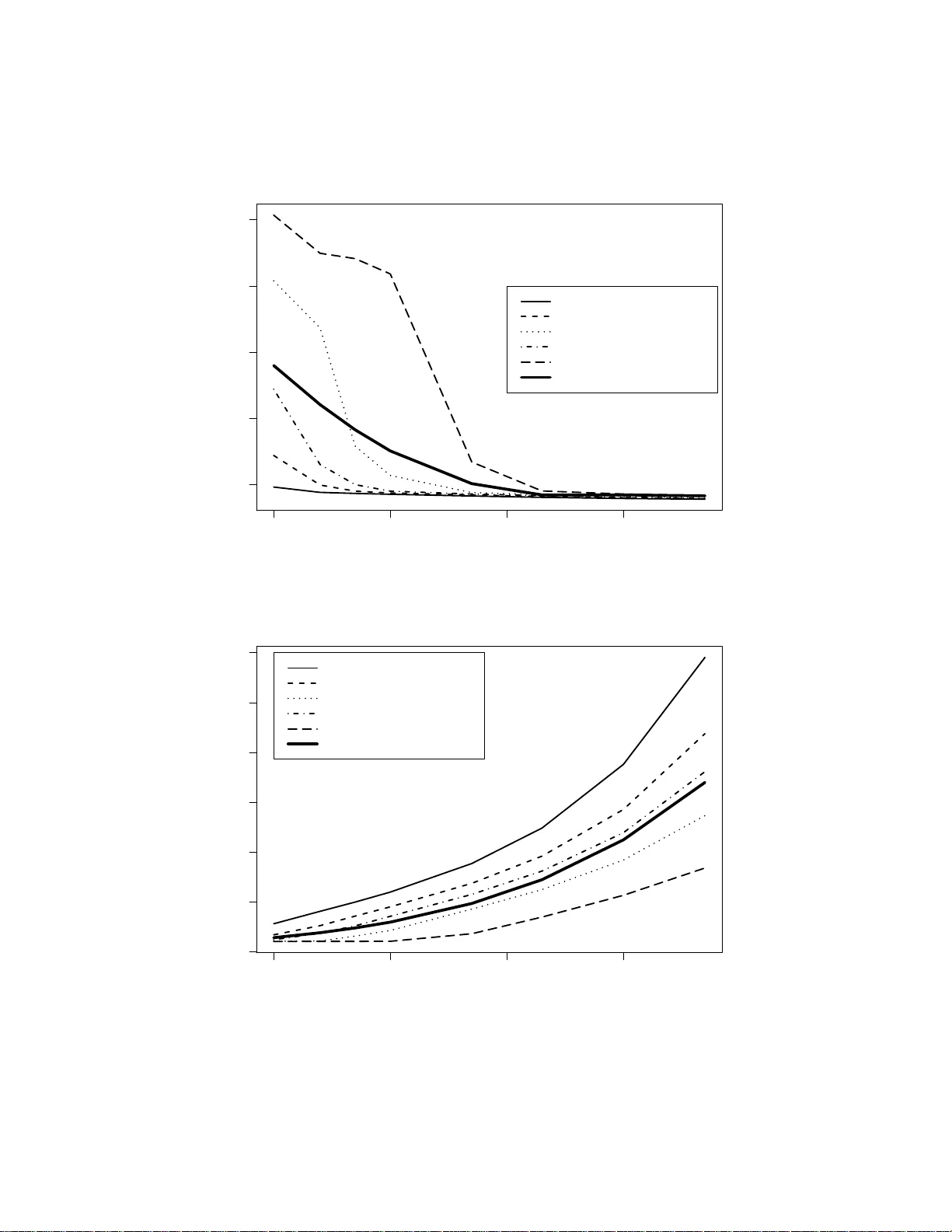
An Empirical Study of Indirect Cross-v alidation Olga Y. Sa v c h uk, Jeffrey D. Hart, Simon J. S hea ther Abstract In this pap er w e pro vide insigh t in to the empirical prop erties of in d irect cross- v a lidation (ICV), a new metho d of bandwid th selection for kernel den s it y estimators. First, w e d escrib e the metho d and rep ort on the theoretical r esults used to d ev elop a pr actical-purp ose mo del for certain ICV p arameters. Next, we pro vide a detailed description of a numerica l stud y whic h sho ws that the ICV metho d us ually outp erforms least squares cross-v a lidation (LSCV) in fin ite samples. One of the ma jor adv an tage s of ICV is its increased stabilit y compared to LSCV. Two real d ata examples sh o w the b enefit of u sing b oth ICV and a lo cal version of ICV. KEY W ORDS: Cross-v alidatio n; Bandwidth selection; Kernel den s it y estimation, In- tegrated Squared E rror, Mean Integrate d Sq u ared Er ror. 1 In tro d u ction Let X 1 , . . . , X n b e a random sample from an unknow n densit y f . A k ernel density estimator of f at the p oin t x is defined as ˆ f h ( x ) = 1 nh n X i =1 K  x − X i h  , (1) where h > 0 is the bandwidth, and K is the kerne l, whic h is generally chose n to b e a unimo dal proba bility densit y function that is symmetric ab o ut zero and has finite v ariance. A p opular c hoice for K is t he Gaussian kerne l: φ ( u ) = (2 π ) − 1 / 2 exp( − u 2 / 2). T o distinguish b et w een estimators with differen t k ernels, w e shall refer to estimator (1) with giv en k ernel K as a K -kernel estimator . 1 Practical implemen tation of the estimator (1) requires specification of the smo othing parameter h . The t w o mo st widely used bandwidth selection metho ds a re least squares cross- v a lidation, pro p osed independen tly b y Rude mo (1 982) and Bo wman (1984), and the Sheather and Jones (19 9 1 ) plug-in metho d. P lug-in is often preferred since it pro duces more stable bandwidths than do es L SCV. Neve rtheless, t he LSCV metho d is still p opular since it requires few er assump- tions than the plug-in metho d and w orks w ell when the densit y is difficult to estimate; see L oader (1999 ), v an Es (1 992), and Sain, Baggerly , a nd Scott (1994 ) . The main flaw of LSCV is high v a r iabilit y o f the selected bandwidths. Other dra wbac ks include the tendency of cross-v alidation curv es to exhibit multiple local minima with the first lo cal minim um b eing to o small (see Hall and Marron (1991 )), a nd the tendency of LSCV to select bandwidths that are m uc h to o small when the data exhibit a small amoun t o f auto correlation (see Hart and Vieu ( 1 990) and Cao and Vilar F ernandez (1993) for res ults of a numerical study ). Man y mo difications of LSCV hav e been prop osed in a n att empt to impro v e it s p erformance. These include biased cross-v a lida t ion of Sc ott and T errell (19 87), a metho d of Chiu (1991), the tr immed cross-v alidation of F eluc h and Koronacki (1992), the mo dified cro ss-v alidation of Stute (1 992), and the metho d o f Ahmad and Ran (20 04) based on ke rnel c ontrasts. This pap er is concerned with a new mo dification of the LSCV metho d, called ind i r e ct cr oss-validation (ICV), recen tly prop osed b y the authors Sa v c h uk, Hart, and Sheather (20 08). The ICV metho d dep ends on tw o parameters, α a nd σ . A main theoretical result is that at asymptotically optimal choices of α and σ the ICV bandwidth can con v erge t o zero at a ra te n − 1 / 4 , whic h is substan tially better than the n − 1 / 10 rate of LSCV . The prese nt pap er con tains the results of an empirical study of ICV. In Section 2 we pro vide a description of the metho d. Section 3 con tains the details underlying the deve lopmen t of a practical purp ose mo del for α and σ . Sec tion 4 outlines the results of a n umerical study which, in particular, sho w that ICV has greater stabilit y in finite samples than do es LSCV. In Section 5 we apply ICV and a lo cal vers ion of ICV to real data sets. Section 6 provides a summary o f our results. 2 2 Descrip t ion of indi rect cross - v alidation 2.1 Notation and definitions W e b egin with some notation and definitions that will b e used subsequen tly . F o r an arbitrary function g , define R ( g ) = Z g ( u ) 2 du, µ j g = Z u j g ( u ) du, where here and subse quen tly integrals are assumed to b e ov er the whole real line. The p opular measures of p erformance of the k ernel estimators (1 ) are in tegrated squared error (ISE) a nd mean in tegrated squared error (MISE). The ISE is defined as I S E ( h ) = Z  ˆ f h ( x ) − f ( x )  2 dx, (2) and MISE is defined as the expectation of ISE. Assuming that the underlying densit y f has second deriv ativ e whic h is contin uous and square in tegrable and that R ( K ) < ∞ , the bandwidth whic h asymptotically minimizes the MISE of the K − k ernel estimator (1) has the follo wing form: h n =  R ( K ) µ 2 2 K R ( f ′′ )  1 / 5 n − 1 / 5 . (3) The LSCV criterion is giv en b y LS C V ( h ) = R ( ˆ f h ) − 2 n n X i =1 ˆ f h, − i ( X i ) , (4) where ˆ f h, − i denotes the k ernel estimator (1) constructed f r o m the data without the obser- v a tion X i . A w ell kno wn fact is that LS C V ( h ) is an un biased estimator of M I S E ( h ) − R f 2 ( x ) dx . F or t his reason t he LSCV metho d is often called unbia se d cr oss-validation . Let ˆ h U C V and h 0 denote the bandwidths which minimize the LSCV function (4 ) and t he M ISE of the φ -kerne l estimator. Section 2.2 defines the ICV bandwidth, denoted as ˆ h I C V . 2.2 The basic metho d The essence o f the ICV metho d is to use different k ernels at the cross-v alidation and density estimation stages. The same idea is exploited by the one-sided cross-v a lidation metho d of Hart and Yi (1 998) in the regression con text. ICV first selects the bandwidth of an L − k ernel es timator using least squares cross-v alida tion. Selection k ernels L used for this purp ose are describ ed in Section 2.3. The bandwidth so obtained is rescaled so that it can 3 b e used with the φ -k ernel estimator. The m ultiplicativ e constan t C has the f ollo wing form: C =  µ 2 2 L 2 √ π R ( L ) 2  1 / 5 , (5) whic h is motiv ated by the asymptotically optimal MISE bandwidth (3 ) . 2.3 Selection k ernels W e consider the family o f k ernels L = { L ( · ; α, σ ) : α ≥ 0 , σ > 0 } , where, for all u , L ( u ; α, σ ) = (1 + α ) φ ( u ) − α σ φ  u σ  . (6) Note that the Gaussian ke rnel is a special case of (6) whe n α = 0 or σ = 1. Eac h member of L is sy mmetric ab out 0 and has the second moment µ 2 L = R u 2 L ( u ) du = 1 + α − α σ 2 . It follo ws that ke rnels in L are second o rder, with the exception of those for whic h σ = p (1 + α ) /α . The family L can b e par t itioned into three fa milies: L 1 , L 2 and L 3 . The first of these is L 1 =  L ( · ; α, σ ) : α > 0 , σ < α 1+ α  . Eac h ke rnel in L 1 has a negative dip cente red at x = 0. The k ernels in L 1 are ones that “cut-out-the- middle,” some examples of which are shown in Figure 1 (a) . The second fa mily is L 2 =  L ( · ; α, σ ) : α > 0 , α 1+ α ≤ σ ≤ 1  . Kernels in L 2 are densities whic h can be unimo dal or bimodal. Note tha t the Gaussian k ernel is a mem b er of this family . The third family is L 3 =  L ( · ; α, σ ) : α > 0 , σ > 1 } , eac h mem b er of whic h has negativ e tails. Examples a r e show n in Figure 1 (b) . Kernels in L 1 and L 3 turn out to b e highly efficien t for cross-v alidation purp oses but very inefficien t for estimating f . This explains wh y w e do not use L as b oth a selection and an estimation kerne l. Selection k ernels in L ar e mixtures of t w o normal densities, whic h greatly simplifies computations. In particular, closed form expressions exist for the LS C V and ISE functions. This fact has b een utilized b y Marron and W and (1992) to deriv e exact MISE expressions. Marron and W and (1992) p o in t out that, in addition to their computational adv an tages, normal mixtures can approximate an y densit y arbitrarily w ell in v arious senses. Mixtures o f normals are therefore an excellen t mo del for use in sim ulation studies, a fact whic h we tak e adv an tage of in Section 4. 4 (a) (b) −4 −2 0 2 4 −1.5 −1.0 −0.5 0.0 0.5 1.0 u L(u) normal alpha=2 alpha=5 −10 −5 0 5 10 −0.5 0.0 0.5 1.0 1.5 2.0 2.5 u L(u) normal sigma=2 sigma=6 Figure 1: ( a) Selection k ernels in L 1 whic h ha v e σ = 0 . 5; (b) Selection kerne ls in L 3 with α = 6. The dotted curv e in b oth gra phs corresp onds to the G aussian ke rnel. 3 Practical issues In this section w e address the problem of ch o osing t he par a meters, α and σ , of the selection k ernel in practice. W e review some large sample theory for the ICV metho d a nd pro vide the theoretical r esults used to dev elop the practical-purp ose mo del for α and σ . 3.1 Large sample theory Large sample theory w as dev elop ed in Sav c huk, Hart, and Sheather (200 8) b y cons idering the asymptotic mean squared error (MSE) of the ICV bandwidth. Their res ults ma y b e summarized a s follows. 1. Under suitable regularit y conditions the ICV bandwidth is asy mptotically normally distributed. 2. The asymptotic MSE of ˆ h I C V has b een found for t w o cases: σ → 0 (cut-out-the- middle ke rnels) and σ → ∞ (negativ e-tailed k ernels). It turns out that when the asymptotically optimal v alues of α and σ are used in the resp ectiv e c ases, the MSE con v erg es to zero at t he same rate of n − 9 / 10 , but the limiting ratio of optim um mean 5 squared errors is 0 . 752, with σ → ∞ yielding the smaller error. In comparison, the rate at whic h the MSE fo r ˆ h U C V con v erg es to zero is n − 6 / 10 . The subsequen t theoretical r esults are provide d for the case σ → ∞ . 3. The relativ e rat e of conv ergence of ˆ h I C V to h 0 is n − 1 / 4 , whereas the corresp onding rate for ˆ h U C V is n − 1 / 10 . 4. V alues of σ whic h minimize the asymptotic MSE a r e as follo ws: σ n,opt = n 3 / 8 A α  R ( f ) R ( f ′′ ) 13 / 5 R ( f ′′′ ) 2  5 / 8 , (7) where A α = 1 6 √ π 2 7 / 16 3 5 / 8 α 3 / 4 (1 + α ) 2  1 8 (1 + α ) 2 − 8 9 √ 3 (1 + α ) + 1 √ 2  5 / 8 . 5. The asym ptotically optimal α is 2 .4233. Remark ably , the optimal α does not dep end on f . 6. When the asymptotically optima l v alues of α and σ are used, the asymptotic bias and standard deviation of ˆ h I C V con v erg e to zero at the same rate of n − 9 / 20 . 3.2 MSE-optimal α and σ Asymptotic res ults are not alwa ys reliable for practical purp oses. In order to hav e an idea of whether the negativ e-ta iled or cut-out- the middle k ernels should really b e used, and ho w go o d c hoices of α and σ v ary with n and f , w e considered the following expression for the asymptotic MSE of the ICV ba ndwidth: MSE( ˆ h I C V ) =  1 4 π  1 / 5 R ( f ′′′ ) 2 R ( f ′′ ) 16 / 5 n − 3 / 5  2 25 R ( f ) R ( f ′′ ) 13 / 5 R ( f ′′′ ) 2 R ( ρ L ) R ( L ) 9 / 5 ( µ 2 2 L ) 1 / 5 + n − 3 / 5 400  R ( L ) 2 / 5 µ 2 L µ 4 L ( µ 2 2 L ) 7 / 5 − 3 (4 π ) 1 / 5  2 ) . (8) Expression (8) is v a lid for either large or small v alues of σ and include s second order bias terms. As our target densities we conside red the follow ing fiv e normal mixtures defined in the article by Marro n and W and (1 992): 6 Densit y sk ew ed separated sk ew ed normal unimo dal bimo dal bimo dal bimo dal n α σ α σ α σ α σ α σ 100 3.05 2.79 5.28 1.6 8 109.68 1.03 16.70 1.19 343.74 1.01 250 2.78 4.04 3.16 2.6 0 48.46 1.06 4.51 1.84 177.15 1.02 500 2.73 4.97 2.84 3.5 6 6.21 1.55 3.18 2.58 161.39 1.02 1000 2.69 5.97 2.75 4.49 3.7 3 2.12 2.84 3.54 123.78 1.03 5000 2.61 8.84 2.66 6.85 2.7 7 4.26 2.70 5.74 4.71 1.79 20000 2.55 12.4 0 2.59 9 .5 8 2.68 6.22 2.63 8.08 2.85 3.46 100000 2.50 18.80 2.53 14.27 2.60 9.19 2 .56 11.94 2.70 5.65 500000 2.47 29.54 2.49 21.88 2.54 13.65 2.50 18.07 2.62 8.39 T able 1: MSE-optimal α and σ . Gaussian densit y: N (0 , 1 ) Sk ewe d unimodal densit y: 1 5 N (0 , 1 ) + 1 5 N  1 2 ,  2 3  2  + 3 5 N  13 12 ,  5 9  2  Bimo dal density : 1 2 N  − 1 ,  2 3  2  + 1 2 N  1 ,  2 3  2  Separated bimo dal densit y: 1 2 N  − 3 2 ,  1 2  2  + 1 2 N  3 2 ,  1 2  2  Sk ewe d bimodal densit y: 3 4 N (0 , 1 ) + 1 4 N  3 2 ,  1 3  2  . These choice s f or f represen t densit y shap es that are common in practice. In T a ble 1 we pro vide the MSE-optimal c hoices of α and σ for the target densitie s at eigh t sample sizes r a nging from n = 100 up to n = 500000 . It is obvious that the MSE-optimal α and σ v ary greatly from one densit y to another, whic h is esp ecially true for “small” sample sizes. Ho w ev er, the o ptimal α seems t o con v erge to a b out 2.5 for eac h densit y as n increases, whic h fits with our observ ation that the optimal α is 2 . 423 3 . The optima l σ is increasing with sample size. It us remark able that all the MSE-optimal α and σ in T able 1 corr esp ond to ke rnels f r o m L 3 , the family of negativ e-tailed k ernels. 3.3 Mo del for the ICV parameters W e found a practical purp ose mo del for α and σ b y using p olynomial regression. Our indep enden t v a r ia ble w a s log 10 ( n ) and our dep endent v ariables we re the MSE-optima l v alues of log 10 ( α ) a nd log 10 ( σ ) fo r differen t densitie s. The log 10 transformations for α and σ stabilize 7 n 100 250 50 0 1000 5000 20000 10 0000 500000 α mod 25.20 12.77 8.24 5.71 3.23 2.6 6 2.66 2.62 σ mod 1.39 1.89 2.37 2.95 4.83 7 .21 11.22 16.98 T able 2: Mo del c hoices of α and σ . v a riabilit y . Using a sixth degree p o lynomial for α and a quadratic fo r σ , w e arriv ed at the follo wing mo dels f or α a nd σ : α mod = 10 3 . 390 − 1 . 093 log 10( n )+0 . 025 log 10( n ) 3 − 0 . 00004 log 10( n ) 6 σ mod = 1 0 − 0 . 58+0 . 386 log 10( n ) − 0 . 012 l og 10( n ) 2 , (9) whic h are appropriate for 100 ≤ n ≤ 5 00000. The MSE-optimal v alues of log 10 ( α ) and σ together with t he mo del fits are sho wn in Figure 2. In T able 2 w e giv e the mo del choices α mod and σ mod for the same sample sizes as in T able 1. 4 Sim ulati on study The primary goal of our simulation study w as to compare ICV with ordinary LSCV. How ev er, w e w ill also pro vide simulation r esults for the Sheather-Jones plug-in metho d. W e considered the four sample sizes n = 100, 25 0 , 500 and 5000, and to ok samples from the target densities listed in Section 3.2. F or each com bination of densit y and sample size w e did 1000 replications. In all cases the parameters α and σ in the selection kerne l L w ere c ho sen a ccording to mo del (9). Let ˆ h 0 denote the minimizer of I S E ( h ) fo r a Gaussian k ernel es timator. F or e ach sam- ple, w e computed ˆ h 0 , ˆ h ∗ I C V , ˆ h U C V and the Sheather-Jones plu g-in bandw idth ˆ h S J P I . The definition of ˆ h ∗ I C V is as follows: ˆ h ∗ I C V = min( ˆ h I C V , ˆ h O S ) , (10) where ˆ h O S is the ov ersmo othed bandwidth of T errell (1990). It is arg ua ble that no da t a - driv en bandwidth should b e larger than ˆ h O S since this statistic estimates a n upp er b ound for al l MISE-optimal bandwidths (under standard smo o thness conditions). F or any ra ndo m v aria ble Y defined in eac h replication o f our sim ulation, we denote the mean, standard deviation and median of Y o v er all replications (with n and f fixed ) by b E( Y ) , c SD( Y ) and d Median( Y ). T o ev aluate the bandwidth selectors w e computed b E  I S E ( ˆ h ) /I S E ( ˆ h 0 )  8 2 3 4 5 0.5 1.0 1.5 2.0 2.5 Model for log10(alpha) log10(n) log10(alpha) normal skewed unimodal bimodal separated bimodal skewed bimodal fit 2 3 4 5 0 5 10 15 20 25 30 Model for sigma log10(n) sigma normal skewed unimodal bimodal separated bimodal skewed bimodal fit Figure 2: MSE-optimal log 10 ( α ) and σ and the mo del fits. 9 n = 100 n = 250 LSCV SJPI ICV ISE 0.1 0.2 0.3 0.4 0.5 0.6 0.7 LSCV SJPI ICV ISE 0.1 0.2 0.3 0.4 0.5 n = 500 n = 500 0 LSCV SJPI ICV ISE 0.1 0.2 0.3 0.4 0.5 LSCV SJPI ICV ISE 0.05 0.10 0.15 0.20 0.25 0.30 Figure 3: Box plots for the data-driv en bandwidths in case of the Normal densit y . and d Median  I S E ( ˆ h ) /I S E ( ˆ h 0 )  for ˆ h equal to eac h of ˆ h ∗ I C V , ˆ h U C V and ˆ h S J P I . W e also com- puted the perfo r ma nce measure b E  ˆ h − ˆ E ( ˆ h 0 )  2 , whic h estimates the MSE of the bandwidth ˆ h . Our main sim ulat ion r esults fo r the “normal” and “bimo dal” densities, a s defined in Section 3.2, are giv en in T ables 3 and 4 and Fig ures 3 and 4. Results for the o t her densities are av ailable from the authors. Ot her statistics rep orted in T ables 3 and 4 are b E( ˆ h ) and c SD( ˆ h ) for eac h t yp e of bandwidth considered. The reduced v ariability of the ICV bandwidth is eviden t in our study . The ratio c SD( ˆ h ∗ I C V ) / c SD( ˆ h U C V ) ranged b et w een 0.9713 and 0.210 3 in the t w en t y settings considered. Ho w ev er, the v ar ia nces of the ICV bandwidths we re alwa ys higher compared to the Sheather-Jones plug-in band- 10 n LSCV SJPI ICV ISE b E( ˆ h ) 100 0.4452 4596 0.3933874 7 0.41530 230 0 .4316231 8 250 0.3639 8008 0.3388353 8 0.34944 737 0 .3548702 9 500 0.3109 4126 0.2980320 5 0.30864 570 0 .3080614 6 5000 0.183 59629 0.1899235 6 0.1976 8683 0 .1952635 8 c SD( ˆ h ) · 10 2 100 12.321 73263 6.432 44579 6. 5229863 7 7.52 008697 250 8.3577 2162 3.7174237 4 4.44775 700 6 .2730032 6 500 7.1116 8918 2.6030098 7 3.08015 801 5 .6349505 9 5000 3.900 77096 0.6190026 8 0.8204 1632 3 .0927742 1 b E( ˆ h − b E( ˆ h 0 )) 2 · 10 4 100 153.52 907115 55.9546 7615 45.17051 435 250 70.611 54173 16.376 60421 20.056 84094 500 50.608 47941 7.774 77660 9. 4812993 6 5000 16.5620 5491 0.667 93916 0.7 3113122 b E  ISE( ˆ h ) / ISE( ˆ h 0 )  100 2.4699 7542 1.9079591 5 1.72178 966 250 1.9159 3730 1.5056301 6 1.47567 596 500 1.7580 6058 1.3773400 3 1.36096 679 5000 1.413 16047 1.1146056 7 1.1031 3807 d Median  ISE( ˆ h ) / ISE( ˆ h 0 )  100 1.3110 8630 1.1569587 6 1.11233 574 250 1.2171 5835 1.1040894 8 1.09365 380 500 1.2139 6609 1.1030640 4 1.09608 944 5000 1.109 07960 1.0447105 5 1.0518 3075 T able 3: Sim ulation results for the Gaussian densit y . 11 n LSCV SJPI ICV ISE b E( ˆ h ) 100 0.429086 86 0.3945343 1 0.419 55286 0.3 8237337 250 0.313609 42 0.3116005 4 0.328 46189 0.2 9715278 500 0.259275 33 0.2623864 6 0.274 50416 0.2 5320682 5000 0.15262 210 0.1570680 4 0.162 55246 0. 1547804 9 c SD( ˆ h ) · 10 2 100 13.565 32316 7.444 25312 9.5668 0379 7.60 899932 250 8.467344 73 4.1877828 8 6.509 18853 4.2 9431763 500 5.705872 08 2.4444330 5 4.200 78840 3.5 5982408 5000 2.46293 965 0.4795175 2 0.814 57083 1. 9650377 7 b E( ˆ h − b E( ˆ h 0 )) 2 · 10 4 100 205.65 547766 56.8403 7076 105.255352 53 250 74.332 44070 19.607 36507 52.12 977298 500 32.892 68754 6.811 93546 22 .164745 97 5000 6.10659 189 0.2820363 7 1.266 89717 b E  ISE( ˆ h ) / ISE( ˆ h 0 )  100 1.699519 29 1.3273359 5 1.361 43018 250 1.515998 57 1.2091414 3 1.287 43335 500 1.416709 96 1.1507089 0 1.191 68891 5000 2.06430 484 1.0683998 7 1.076 75906 d Median  ISE( ˆ h ) / ISE( ˆ h 0 )  100 1.209515 75 1.0874416 1 1.133 56965 250 1.160878 96 1.0833897 0 1.126 99702 500 1.122436 94 1.0607270 2 1.094 21867 5000 1.05825 025 1.0306796 3 1.036 49944 T able 4 : Sim ulation results for the Bimo dal densit y . 12 n = 100 n = 250 LSCV SJPI ICV ISE 0.2 0.4 0.6 0.8 LSCV SJPI ICV ISE 0.1 0.2 0.3 0.4 0.5 n = 500 n = 500 0 LSCV SJPI ICV ISE 0.05 0.10 0.15 0.20 0.25 0.30 0.35 0.40 LSCV SJPI ICV ISE 0.00 0.05 0.10 0.15 0.20 Figure 4: Bo xplots f or the data-driven bandwidths in case of the Bimo dal densit y . 13 0.0 0.1 0.2 0.3 0.4 0 2 4 6 8 10 h density estimates LSCV ICV ISE Figure 5: Kernel dens ity estimates f o r random bandwidths from the sim ulation with the Sk ewe d Unimodal densit y and n = 25 0. widths. It is w o rth noting that the ratio of sample standar d deviations of the ICV and LSCV bandwidths decreases a s the sample size n increases. The mean squared distance b E  ˆ h − b E( ˆ h 0 )  2 w a s smaller f or the ICV metho d tha n for the LSCV method in all but t w o cases corres p onding to the Sk ew ed Bimo dal dens ity , n = 250 and 500. Plug-in alwa ys had a smaller v alue of b E  ˆ h − b E( ˆ h 0 )  2 than did ICV. The most imp ortant observ atio n is that the v alues o f b E  I S E ( ˆ h ) /I S E ( ˆ h 0 )  w ere smaller for ICV than for LSCV fo r all combinations of den sities and sample sizes . The v a lues of d Median  I S E ( ˆ h ) /I S E ( ˆ h 0 )  w ere smaller for ICV than fo r LSCV in all but one case, whic h corresp onds to the Sk ew ed Bimo dal densit y at n = 250 when d Median  I S E ( ˆ h I C V ) /I S E ( ˆ h 0 )  w a s 1.0013 times greater than d Median  I S E ( ˆ h U C V ) /I S E ( ˆ h 0 )  . Despite the fact that the LSCV ba ndwidth is asymptotically normally distributed (see Hall a nd Marro n ( 1 9 8 7 ) ) , its distribution in finite samples tends to b e sk ew ed to the left. In our simulations w e hav e noticed that the distribution of the ICV bandwidth is less sk ew ed t ha n that of the LSCV bandwidth. A t ypical case is illustrated in Figure 5, where k ernel de nsit y estimates for the t w o data- driv en bandwidths a r e plotted from the simulation with t he Sk ew ed Unimo da l den- sit y at n = 250. Also plot ted is a dens ity estimate for the ISE-optimal bandwidths. Note that the IC V den sit y is more conce ntrated near the middle of the ISE-optimal distribution than the densit y estimate for LSCV. Figure 6 pro vides scatterplots of the bandwidths ˆ h U C V and ˆ h I C V v ersus ˆ h 0 in the case 14 (a) (b) 0.2 0.3 0.4 0.5 0.10 0.15 0.20 0.25 0.30 0.35 0.40 h.ise h.lscv 0.2 0.3 0.4 0.5 0.10 0.15 0.20 0.25 0.30 0.35 0.40 h.ise h.wcv Figure 6: Scatterplots of ˆ h vs. ˆ h 0 for the case of a Gaussian dens ity and n = 500, with ˆ h corresp onding to the (a) LSCV and ( b) ICV bandwidths. of the G aussian densit y and n = 50 0. The sample correlation co efficien ts w ere -0.52 and -0.60 for LSCV and ICV, res p ectiv ely . The fact tha t these correlations are negativ e is a w ell- established phenomenon; see, for example, Hall a nd Johnstone (1992). Note that the ICV bandwidths cluster more tigh tly ab out the MISE minimizer h 0 = 0 . 315 . A problem w e hav e noticed w ith the ICV metho d is that its criterion function c an hav e t w o lo cal minima when the sample size is mo derate and the densit y has t w o mo des. The follo wing example illustrates the problem. In Figure 7(a) we hav e plotted three ICV curve s for the case o f the Separated Bimo dal densit y a nd n = 100. The minimizers of the solid, dashed and dotted lines occur at the h -v alues 0.2991, 2.0467 and 0.2204, resp ectiv ely . F or comparison, the corresp onding bandwidths chosen b y the Sheather-Jones plug-in metho d are 0.3240, 0.2508 and 0.2467. The v a lue of h = 2 . 0467 whic h minimizes the da shed ICV curv e is ob viously t o o large. The lo cal minim um at 0.1295 w ould yield a m uc h more reasonable estimate. The problem of ch o osing to o large a bandwidth fr om the second lo cal minim um is mitigated b y using the rule ( 10). Indeed, the o v ersmo othed bandwidths for the three samples are sho wn b y the v ertical lines in Figure 7 and w ere 0 .7404, 0.7580 and 0 .7341. Note that the problem with the ICV curve ha ving tw o lo cal minima of approxim ately the same v alue quic kly go es a w a y a s the sample size increases. This is illustrated in Figure 7 ( b) , whe re w e ha v e plo tted three criterion curve s for t he Separated Bimo dal case with n = 500. Th us, t he selection rule ˆ h ∗ I C V giv en b y (10) rather than just ˆ h I C V app ears to b e useful mostly f or small and mo derate sample sizes. 15 (a) (b) 0.0 0.5 1.0 1.5 2.0 2.5 3.0 1 2 3 4 ICV criterion functions h criterion 0 1 2 3 4 0.0 0.5 1.0 1.5 ICV criterion functions h criterion Figure 7: Three ICV criterion functions in case of the Separated Bimodal densit y at (a) n = 100 and (b) n = 5 0 0. 5 Real data examples In t his section w e sho w ho w the IC V method w orks on t w o real data sets. The purpo se of t he first example is t o compare the p erformance of the ICV, LSCV, and Sheather-Jones plug-in metho ds. The second example illustrates the b enefit of using ICV lo cally . 5.1 PGA data In this example the data a re the av erage n um b ers of putts per round pla y ed, fo r the top 175 play ers on t he 1980 and 2 001 PGA golf to urs. The question of interes t is whether there has been any impro v emen t from 1980 to 2001. This data set has a lready b een analyzed b y Sheather (2 004) in the contex t of comparing the p erformances of LSCV and Sheather- Jones plug-in. In Figure 8 w e hav e plot t ed an unsmoothed frequency histogram and the LSCV, ICV and Sheather-Jones plug-in density estimates fo r a com bined data set of 1 980 and 2001 putting a v erages. The class in terv al size in the unsmo ot hed histogram w a s chos en to b e 0 .01, whic h corresp onds to the accuracy to whic h the data hav e b een reported. There is a clear indication of tw o mo des in the histogram. The es timate based on the LSC V bandwidth is apparen tly undersmo othed. The ICV and plug- in estimates lo ok similar and hav e tw o mo des, whic h agrees with evidence from the unsmo othed histogram and seems reasonable since the data w ere tak en from t w o p opulations. 16 Unsmoothed frequency histogram Average number of putts 27 28 29 30 31 32 33 0 1 2 3 4 5 6 27 28 29 30 31 32 33 0.0 0.2 0.4 0.6 0.8 LSCV density estimate Average number of putts Density estimate h_LSCV= 0.0532 27 28 29 30 31 32 33 0.0 0.2 0.4 0.6 0.8 ICV density estimate Average number of putts Density estimate h_ICV= 0.1977 27 28 29 30 31 32 33 0.0 0.2 0.4 0.6 0.8 SJ plug−in density estimate Average number of putts Density estimate h_SJPI= 0.1544 Figure 8: Unsmo othed frequency histogram a nd k ernel dens ity estimates for a v erage num b ers of putts p er round from 19 80 and 2001 com bined. In Figure 9 w e hav e plotted k ernel densit y estimates separately for the ye ars 1980 and 2001. ICV seems to pro duce a reasonable estimate in b oth y ears, whereas LSCV yields a v ery wiggly and apparen tly undersmo othed estimate in 2001. 5.2 Lo cal ICV example Lo cal cross-v alidation methods for density estimation, indep enden tly prop o sed by Hall and Sch ucan y (1 989) and Mielniczuk, Sarda, and Vieu (198 9), consist in p erforming L SCV at eac h v alue of the argumen t x usin g a fraction of the data that are close to x . Allo wing the bandwidth to dep end on x is desirable when the smo o thness o f the underlying density ch anges sufficien tly with x . 17 28 29 30 31 32 0.0 0.2 0.4 0.6 0.8 1.0 1.2 Average Number of Putts Estimated density 2001 1980 h_ICV= 0.1791 (2001) h_LSCV= 0.0617 (2001) h_ICV= 0.1518 (1980) h_LSCV= 0.1874 (1980) Figure 9: Kernel densit y estim ates ba sed on LSCV (dashed curv e) a nd ICV (solid curve ) pro duced separately fo r the data from 1 980 and 2001. The lo cal ICV method w as in tro duced in Sa v c h uk, Hart, and Sheather ( 2 008). It is dif- feren t from the lo cal LSCV metho d in that it uses ICV rather than LSCV for the lo cal bandwidth selection. Another difference is that lo cal ICV uses the first lo cal minimizer of the lo cal criterion function as opp osed to the global minimizer of lo cal LSCV. The lo cal ICV criterion function is defined as I C V ( x, b, w ) = 1 w Z φ  x − u w  ˆ f b ( u ) 2 du − 2 nw n X i =1 φ  x − X i w  ˆ f b, − i ( X i ) , where function ˆ f b is the k ernel densit y estimate based on a selection ke rnel L with a smo ot h- ing para meter b . The quan tity w defines the exten t to whic h the cross-v alidatio n is lo cal, with a large c hoice of w corresp onding to glo ba l ICV. Let ˆ b ( x ) b e the first lo cal mini- m um of the lo cal ICV curve for the fixed v alue of x . Then the corres p onding bandwidth 18 (a) (b) −200 0 200 400 600 800 1000 0.000 0.001 0.002 0.003 0.004 ICV density estimate x −200 0 200 400 600 800 1000 0.000 0.001 0.002 0.003 0.004 Local ICV estimate x Figure 10 : Densit y estimates for the DC data set with (a) b eing the global ICV densit y estimate and (b) corresp onding to the lo cal ICV estimate. of a φ − k ernel estim ator is defined as ˆ h ( x ) = C ˆ b ( x ), whe re C is compute d as in (5). Lo- cal ICV o utp erformed the lo cal LSCV metho d in a s im ulated data example in the article of Sa v c h uk, Hart, and Sheather (2008). In this pap er w e sho w ho w lo cal ICV and LSCV p erform in a real data example. W e a nalyze t he data of size n = 517 on the Droug h t Co de (DC) of the Canadian F orest Fire W eather index (FWI) sy stem. D C is one of the explanatory v ariables wh ic h can be used to predict the burned a r ea of a forest in the F orest Fires data set. This data can b e do wnloaded from the w ebsite http://arc hive.ics.uci.edu/ml/datasets/Forest+Fires . The data we re collected and a nalyzed by Cortez and Morais (2007). W e computed the LSC V, ICV and Sheather-Jones plug-in bandwidths for the DC data. The LSCV metho d fa iled b y yielding ˆ h U C V = 0. ICV and Sheather-Jones plug-in bandwidths w ere v ery close and pro duced similar density estimates. Figure 10 (a) giv es t he ICV densit y estimate. It shows tw o ma j o r mo des connected with a wiggly curv e, whic h indic ates that v a rying the bandwidth with x may yield a smo o ther estimate of the underlying densit y . Lo cal ICV and LSCV ha v e b een applied to the DC data. W e us ed w = 40 for bo th metho ds and the selection k ernel with α = 6 a nd σ = 6 for lo cal ICV. This ( α, σ ) choic e p erformed quite w ell for unimo dal densities in our simulation studies o n global ICV, a nd hence seems to b e reasonable for lo cal bandwidth se lection since lo cally the de nsit y should ha v e relative ly few features. Let x ( i ) , i = 1 , . . . , n , de note the i th mem b er of the ordered sequence o f observ ations. The lo cal IC V and LSCV bandwidth w ere found f o r 50 ev enly 19 spaced p oin ts in the interv al x (1) − 0 . 2 ( x ( n ) − x (1) ) ≤ x ≤ x ( n ) + 0 . 2( x ( n ) − x (1) ). It t ur ns out that in 45 out of 50 cases the lo cal LSCV curv e tends to −∞ a s h → 0, whic h implies that the lo cal L SCV estimate can not b e computed. All 50 lo cal ICV bandwidths w ere p ositiv e. W e found a smo oth func tion ˆ h ( x ) b y inte rp olat ing at o ther v a lues of x via a spline. The corresp onding lo cal ICV estimate, given in Figure 10 (b) , sho ws a smo other densit y estimate. 6 Summary Indirect cross-v alidation is a metho d of bandwidth selection in the univ ariate k ernel densit y estimation contex t. T he me tho d first selects the bandwid th of an L − k ernel estimator b y least squares cross-v alidation, and then rescales this bandwidth so that it is appropriate for use in a Gaussian kerne l dens ity estimator. Selection ke rnels L ha v e the form (1+ α ) φ ( u ) − αφ ( u/ σ ) /σ , where α ≥ 0, σ > 0 and φ is the Ga ussian k ernel. Optimal k ernels from this class yield bandwidths with relative error that con v erges to 0 a t a rate of n − 1 / 4 , whic h is a substan tial impro v emen t o ver the n − 1 / 10 rate of LSCV. A pr a ctical purp o se mo del for the selection kerne l parameters, α and σ , has b een dev el- op ed. The mo del was built by p erforming p olynomial regression on the MSE-optimal v a lues of log 10 ( α ) and log 10 ( σ ) at differen t sample sizes fo r fiv e ta rget densities. Use of this mo del mak es the ICV metho d completely automatic. An extens iv e sim ulation study sho w ed that in finite samples ICV is more stable than LSCV. Although b oth ICV and LSCV bandwidths are asymptotically normal, the distribu- tion of the ICV bandwidth for finite n is usually more symmetric and b etter concentrated in the middle of the den sit y for ISE-optimal bandwidths. Using an o ve rsmo othed bandwidth as an upp er b ound for the bandwidth searc h in terv al red uces the bias of the metho d and prev ents selecting an impractically large v alue of h when the criterion curv es exhibit m ultiple lo cal minima. The ICV metho d p erforms we ll in real data examples. ICV a pplied lo cally yields densit y estimates which are more smo oth tha n estimates based on a single bandwidth. Often, lo cal ICV estimates may b e found when the lo cal LSCV estimates do not exist. References Ahmad, I. A. and I. S. Ran (2004 ). Kernel contrasts: a data-based metho d of c ho os- ing smo othing parameters in nonparametric densit y estimation. J. Nonp ar ametr. 20 Stat. 1 6 (5), 671– 7 07. Bo wman, A. W. (1984). An alternativ e metho d of cross-v alidation for the smo othing of densit y es timates. Biom etrika 71 (2), 3 53–360. Cao, R ., Q. d. R. A. and J. Vilar F ernandez ( 1993). Bandwidth selection in nonpara metric densit y estimation under dep endence : a simulation study . C omputational Statistics 8 , 313– 332. Chiu, S.-T. (1991 ) . Ba ndwidth selection fo r k ernel densit y estimation. Ann. Statist. 19 (4), 1883–190 5. Cortez, P . and A. Morais (2007) . A data mining approac h to predict for est fires using meteorological data. in J. Neves, M. F. Santos and J. Machado Eds., New T r ends in A rtificial Intel ligen c e, Pr o c e e d ings of the 13 th EPIA 2007 - Portuguese Con f e r e nc e on A rtificial Intel li g enc e, De c em b er, Guimar aes, Portu gal , 512–5 2 3. F eluc h, W. and J. Koronack i (1992). A note on mo dified cross -v alidatio n in dens it y esti- mation. Comput. Statist. Data A nal. 13 (2 ) , 143–151. Hall, P . and I. Johnstone (1992). Empirical functional and efficien t s mo othing para meter selection. J. R o y. Statist. So c. Ser. B 54 (2), 475–5 30. With discussion and a reply by the a ut ho rs. Hall, P . and J. S. Marron (198 7). Exten t to which least-squares cross-v alidation minimises in tegrated square error in nonparametric densit y estimation. Pr ob ab. The ory R elate d Fields 74 (4), 5 67–581. Hall, P . and J. S. Marro n (1991 ) . Lo cal minima in cross-v alidation functions. J. R oy. Statist. So c. Se r. B 53 (1) , 245–252. Hall, P . and W. R. Sc h ucan y (19 8 9). A local cross-v alida t io n algorithm. Statist. Pr o b ab. L ett. 8 (2), 109–1 17. Hart, J. D. and P . Vieu (1990). Data-driv en bandwidth c hoice for densit y estimation based on dep enden t data . Ann. Statist. 18 (2), 873–890. Hart, J. D . and S. Yi (1 998). One-sided cross-v alidation. J. A mer. Statist. Asso c. 93 (442), 620–631. Loader, C. R. (1 9 99). Bandwidth selection: classical or plug-in? A nn. Statist. 27 (2), 415–438. Marron, J. S. and M. P . W and (1992). Exact mean in tegrated squared error. Ann. Statist. 20 (2), 712–7 36. 21 Mielniczuk, J., P . Sarda, and P . Vieu (1989). Lo cal data-driv en bandwidth c hoice for densit y es timation. J. Statist. Plann. Infer enc e 23 (1), 53–69. Rudemo, M. (198 2). Empirical c hoice of histog rams a nd k ernel densit y estimators. Sc and. J. Statist. 9 (2), 65 –78. Sain, S. R., K. A. Baggerly , and D. W. Scott (1994). Cross-v alidation of m ultiv ariate densities. J. Amer. Statist. Asso c. 89 (42 7 ), 807–817. Sa v c h uk, O. Y., J. D. Hart, and S. J. Sheather (200 8). Indirect cro ss-v alidat ion fo r densit y estimation. J. Amer. Statist. Asso c., submitt e d . Scott, D. W. and G . R. T errell (19 8 7). Biased and unbiased cross-v alidation in densit y estimation. J. Amer. Statist. Asso c. 82 (400) , 1131–1146 . Sheather, S. J. (2004). Densit y estimation. Statist. Sci. 19 ( 4), 588– 597. Sheather, S. J. and M. C. Jones (1991). A reliable data-based bandwidth selection metho d for kerne l dens ity estimation. J. R oy. Statist. So c. Ser. B 5 3 (3), 6 8 3–690. Stute, W. (1992) . Mo dified cross-v alidatio n in densit y estimation. J. S tatist. Plann. Infer- enc e 30 (3), 29 3 –305. T errell, G. R. ( 1990). The maximal sm o ot hing principle in densit y estimation. J. A mer. Statist. A sso c . 85 (410), 470 –477. v a n Es, B. (1 9 92). Asymptotics f or least squares cross-v alidation bandwidths in nonsmo oth cases. Ann. Statist. 20 (3), 1647 – 1657. 22