Indirect Cross-validation for Density Estimation

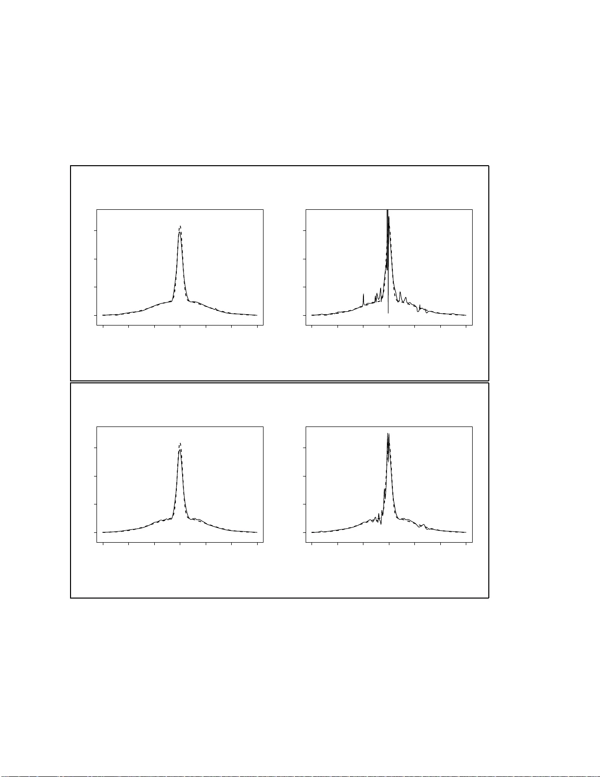
Indirect Cross-v alidation for Densit y Estimation Olga Y. Sa v c h uk, Jeffrey D. Hart, Simon J. S hea ther Abstract A new metho d of bandwidth se lection f or kernel densit y estimators is prop osed. The metho d, termed indir e ct cr oss-validation , or ICV, mak es use of so-called sele c tion k ernels. Least squares cross-v alidation (LSCV) is used to select the bandwidth of a selectio n-kernel estimator, and this bandwid th is appropriately rescale d for use in a Gaussian k ernel estimator. The prop osed selection k ernels are linear com binations of t wo Gaussian k ernels, and need not b e unimo dal or p ositive . Theory is deve lop ed sh o w ing that the relativ e error of ICV bandwid ths can conv erge to 0 at a rate of n − 1 / 4 , which is substan tially b etter than the n − 1 / 10 rate of LS CV. Interestingly , the selection k ernels that are b est for purp oses of bandwid th s electi on are very p o or if used to actually estimate the densit y function. Th is pr op ert y app ears to b e part of the larger and w ell-docum en ted parado x to the effect that “the harder th e estimation problem, the b etter cross-v alidation p erforms.” The ICV metho d uniformly outp erforms LSC V in a simulati on study , a real data example, and a sim ulated example in wh ich b andwidths are c hosen lo cally . KEY W ORDS: Kernel densit y estimati on; Bandwidth sele ction; Cross-v alidation; Lo cal cross-v alidation. 1 1 In t ro du ction Let X 1 , . . . , X n b e a random sample f rom an unkno wn densit y f . A kerne l densit y estimator of f ( x ) is ˆ f h ( x ) = 1 nh n X i =1 K  x − X i h  , (1) where h > 0 is a smo o thing parameter, a lso known as the bandwidth, and K is the k ernel, whic h is generally c hosen to b e a unimo dal probabilit y densit y function that is symmetric ab out zero and has finite v ar ia nce. A p opular choice for K is the Ga us- sian k ernel: φ ( u ) = (2 π ) − 1 / 2 exp( − u 2 / 2). T o distinguish b et w een estimators with differen t k ernels, we shall refer to estimator (1 ) with giv en k ernel K as a K -kernel estimator . Cho osing an a ppro priate bandwidth is vital for the go o d p erfo r ma nce of a k ernel estimate. This pap er is concerned with a new metho d of data-driv en bandwidth selection that w e call indir e ct cr os s -validation (ICV). Man y data-driv en metho ds of ba ndwidth selec tion hav e b een prop osed. The t w o most widely used are least squares cross-v alidation, prop o sed indep enden tly b y Rudemo (1982) and Bowman (1984), and the Sheather and Jones (199 1) plug-in metho d. Plug-in pro duces more stable bandwidths than do es cross-v alidatio n, and hence is the curren tly more p o pular metho d. Nonetheless, an arg ument can b e made for cross-v alidation since it requires few er assumptions tha n plug- in and w orks well when the densit y is difficult to estimate; see Loader (1999). A surv ey of bandwidth selection metho ds is giv en b y Jones, Marron, and Sheather (1996). A num b er o f mo difications of LSCV has b een prop osed in an attempt t o improv e its p erformance. These include the biased cross-v a lidation metho d of Scott a nd T errell (1987), a metho d of Chiu (19 9 1a), the t rimmed cross-v alidation of F eluc h and Ko r onac ki (1992), the mo dified cross-v alidatio n of Stute (1992), and the metho d of Ahmad a nd Ra n (2004) based on k ernel con tra sts. The ICV method is similar in spirit to one-sided cross- 2 v alidation (OSCV), whic h is another mo dification of cross-v alida tion prop osed in the regression context b y Hart and Yi (1998 ). As in OSCV, ICV initially choo ses the bandwidth of an L -k ernel estimator using least squares cross-v alidation. Multi- plying the bandwidth c hosen at this initial stage b y a kno wn constan t results in a bandwidth, call it ˆ h I C V , that is appropriate for use in a Gaussian kerne l estimator. A p opular means of judging a k ernel estimator is the mean integrated squared error, i.e., M I S E ( h ) = E [ I S E ( h )], where I S E ( h ) = Z ∞ −∞  ˆ f h ( x ) − f ( x )  2 dx. Letting h 0 b e t he bandwidth that minimizes M I S E ( h ) when the kernel is Gaussian, w e will sho w t ha t the mean squared error of ˆ h I C V as an estimator of h 0 con v erges to 0 a t a faster rate than that of the ordinary LSCV bandwidth. W e also describe an unexp ected b on us asso ciated with ICV, namely t ha t , unlik e LSCV, it is robust to rounded data. A fairly extensiv e simulation study and t w o data a na lyses confirm that ICV p erfor ms b etter than ordinary cross-v alida t io n in finite samples. 2 Descrip tion of in direct cros s-v alidation W e b egin with some nota tion and definitions that will b e used subsequen tly . F or an arbitrary function g , define R ( g ) = Z g ( u ) 2 du, µ j g = Z u j g ( u ) du. The LSCV criterion is giv en by LS C V ( h ) = R ( ˆ f h ) − 2 n n X i =1 ˆ f h, − i ( X i ) , 3 where, f or i = 1 , . . . , n , ˆ f h, − i denotes a ke rnel estimator using all the original obser- v ations except fo r X i . When ˆ f h uses k ernel K , LS C V can b e written as LS C V ( h ) = 1 nh R ( K ) + 1 n 2 h X i 6 = j Z K ( t ) K  t + X i − X j h  dt − 2 n ( n − 1) h X i 6 = j K  X i − X j h  . (2) It is w ell kno wn that LS C V ( h ) is an unbiased estimator of M I S E ( h ) − R f 2 ( x ) dx , and hence the minimizer of LS C V ( h ) with r espect to h is denoted ˆ h U C V . 2.1 The basic metho d Our aim is to c ho ose the bandwidth of a se c ond or der k ernel estimator. A second order k ernel in tegrates to 1, has first momen t 0, and finite, nonzero second momen t. In principle o ur metho d can b e used to ch o ose the bandwidth of an y second order k ernel estimator, but in this a r t icle w e restrict atten tion to K ≡ φ , the Gaussian k ernel. It is w ell kno wn tha t a φ -k ernel estimator has asymptotic mean integrated squared error (MISE) within 5% of the minim um among all p o sitiv e, second order k ernel estimators. Indirect cross-v alidation ma y b e describ ed as follows : • Select the bandwidth of an L -kerne l estimator using least squares cross-v al- idation, and call this bandwidth ˆ b U C V . The k ernel L is a second order kernel that is a linear combination of tw o G a ussian kernels , and will b e discusse d in detail in Section 2 .2. • Assuming that the underlying densit y f has second deriv ativ e whic h is con- tin uous and square in tegrable, the ba ndwidths h n and b n that asymptotically minimize the M I S E of φ - and L - kernel estimators, respectiv ely , are related 4 as follows : h n = R ( φ ) µ 2 2 L R ( L ) µ 2 2 φ ! 1 / 5 b n ≡ C b n . (3) • Define the indirect cross-v alidat io n bandwidth b y ˆ h I C V = C ˆ b U C V . Imp or- tan tly , the constan t C dep ends on no unkno wn parameters. Express ion (3) and existing cross-v alidation theory suggest that ˆ h I C V /h 0 will at least con- v erge to 1 in probability , where h 0 is the minimizer of M I S E for the φ -kerne l estimator. Henceforth, w e let ˆ h U C V denote t he bandwidth that minimizes LS C V ( h ) with K ≡ φ . Theory of Hall and Marron (19 87) and Scott and T errell (19 8 7) sho ws that the relative error ( ˆ h U C V − h 0 ) /h 0 con v erges to 0 at t he rather disapp ointing r a te of n − 1 / 10 . In con trast, we will show that ( ˆ h I C V − h 0 ) /h 0 can con v erge to 0 at the rate n − 1 / 4 . Kernels L that are sufficien t for this result are discussed next. 2.2 Selection k ernels W e consider the family of k ernels L = { L ( · ; α , σ ) : α ≥ 0 , σ > 0 } , where, for all u , L ( u ; α, σ ) = (1 + α ) φ ( u ) − α σ φ  u σ  . (4) Note that the Gaussian kernel is a sp ecial case of (4) when α = 0 or σ = 1. Eac h mem b er of L is symmetric a b out 0 and such that µ 2 L = R u 2 L ( u ) du = 1 + α − ασ 2 . It fo llo ws that k ernels in L are second order, with the exception of those for whic h σ = p (1 + α ) /α . The family L can b e partitioned in to three families: L 1 , L 2 and L 3 . The first of these is L 1 =  L ( · ; α, σ ) : α > 0 , σ < α 1+ α  . Eac h k ernel in L 1 has a nega t iv e dip cen tered a t x = 0. F or α fixed, the smaller σ is, the more extreme the dip; and for 5 −10 −5 0 5 10 −0.5 0.0 0.5 1.0 1.5 2.0 2.5 u L(u) normal sigma=2 sigma=6 Figure 1: Selection k ernels in L 3 . The dotted curv e corresp onds to the Gaussian k ernel, and each of the other k ernels has α = 6. fixed σ , the larg er α is, the more extreme the dip. The k ernels in L 1 are o nes that “cut-out-the-middle.” The second fa mily is L 2 =  L ( · ; α, σ ) : α > 0 , α 1+ α ≤ σ ≤ 1  . Kernels in L 2 are densities whic h can b e unimo dal or bimo dal. Note t ha t the Gaussian k ernel is a mem b er of this family . The third sub-family is L 3 =  L ( · ; α, σ ) : α > 0 , σ > 1 } , eac h mem b er of whic h has negativ e t a ils. Examples of k ernels in L 3 are sho wn in Figure 1. Kernels in L 1 and L 3 are not of the type usually used for estimating f . Nonethe- less, a w orth while question is “why not use L for b oth cross-v alidation an d estimation of f ?” One could then b ypass the step of rescaling ˆ b U C V and simply estimate f b y an L -k ernel estimator with bandwidth ˆ b U C V . The ironic answ er to this question is t ha t the k ernels in L t ha t are b est for cross-v alidatio n purp oses a r e very inefficien t for estimating f . Indeed, it turns o ut that an L -k ernel estimator based on a sequence 6 of ICV-optimal k ernels has M I S E that do es not conv erge to 0 faster than n − 1 / 2 . In con trast, the M I S E of the b est φ -k ernel estimator tends to 0 lik e n − 4 / 5 . These facts fit with other cross-v a lidation paradoxes, whic h include the fact t ha t LSCV outp erforms other metho ds when the densit y is highly structured, Loader (199 9 ), the improv ed p erformance of cross-v alidat io n in m ultiv ariate densit y estimation, Sain, Baggerly , and Scott (1994 ), and its improv emen t when the true densit y is not smo oth, v a n Es (1992). One could pa r a phrase these phenomena as follows : “The more difficult the function is to estimate, the b etter cross-v alidation seems to p er- form.” In our w ork, we hav e in essence made the function more difficult to estimate b y using an inefficien t k ernel L . More details on the M I S E of L -k ernel estimators ma y b e found in Sav c h uk (2009). 3 Large sample theory The theory presen ted in this section provides the underpinning fo r our metho dology . W e first state a theorem on the asymptotic distribution of ˆ h I C V , and then deriv e asymptotically optimal c hoices for the par a meters α and σ of the selection k ernel. 3.1 Asymptotic mean squared error of the ICV bandwidth Classical theory of Ha ll and Marron (1 9 87) and Scott and T errell (1987) entails that the bia s of an LSCV bandwidth is asymptotically negligible in comparison to its standard deviation. W e will show that the v ariance of an ICV bandwidth can con v erge to 0 at a f aster rate than that of an LSCV bandwidth. This comes at the exp ense of a squared bias that is n o t negligible. How ev er, w e will show how to select α and σ (the parameters of the selection k ernel) so tha t the v ariance and squared bias are balanced and the resulting mean squared error tends to 0 at a fa ster rate 7 than do es that of the LSCV bandwidth. The optimal rate of con v ergence of t he relativ e erro r ( ˆ h I C V − h 0 ) /h 0 is n − 1 / 4 , a substan tial improv emen t ov er the infamous n − 1 / 10 rate for LSCV. Before stating our main result concerning the asymptotic distribution of ˆ h I C V , w e define some notation: γ ( u ) = Z L ( w ) L ( w + u ) du − 2 L ( u ) , ρ ( u ) = uγ ′ ( u ) , T n ( b ) = X X 1 ≤ i 2 K (0), re - sp ectiv ely . The former condition holds necessarily if K is nonnegative and has its maxim um at 0. This means that all the traditional k ernels hav e t he problem of c ho osing h = 0 when the da t a are r o unded. Recall that selection ke rnels (4) a r e not restricted to b e nonnegative. It turns out that there exist α and σ suc h that R ( L ) > 2 L (0 ) will hold. W e sa y that selection k ernels satisfying this condition are ro bust to rounding. It can b e verifie d that the negativ e-tailed selection k ernels with σ > 1 a re robust to rounding when α > − a σ + q a σ + (2 − 1 / √ 2) b σ b σ , (12) where a σ =  1 √ 2 − 1 √ 1+ σ 2 − 1 + 1 σ  and b σ =  1 √ 2 − 2 √ 1+ σ 2 + 1 σ √ 2  . It turns out that all the selection k ernels corresp onding to mo del ( 1 1) are robust to rounding. Figure 2 shows the region (12) and also the curv e defined b y mo del (11) for 1 00 ≤ n ≤ 500 000. Intere stingly , the b o undary separating robust from nonrobust k ernels almost coincides with the ( α, σ ) pa irs defined b y that mo del. 6 Lo c al ICV A lo cal v ersion o f cro ss-v a lida tion f or densit y estimation was prop o sed a nd analyzed indep enden tly by Hall and Sch ucan y (19 89) and Mielniczuk, Sarda, and Vieu (1989). 13 5 10 15 20 5 10 15 20 25 30 sigma alpha n=100 n=500000 Figure 2: Selection k ernels ro bust to rounding ha v e α a nd σ ab o v e the solid curv e. Dashed curv e corresp onds to the mo del-ba sed selection k ernels. A lo cal metho d allows the bandwidth to v ar y with x , whic h is desirable when the smo othness of the underlying densit y v aries sufficien tly with x . F an, Hall, Martin, and Patil (1996) prop osed a differen t metho d of lo cal smo othing that is a hybrid of plug-in and cross- v alidation metho ds. Here we pro p ose that ICV b e p erformed lo cally . The metho d parallels tha t o f Hall a nd Sc h ucan y (1989) and Mielniczuk, Sarda, and Vieu (1989), with the main difference b eing that eac h lo cal bandwidth is c hosen b y ICV rather than LSCV. W e suggest using the sma l l e s t lo cal minimizer o f the ICV curv e, since ICV do es not hav e LSCV’s tendency to undersmo oth. Let ˆ f b b e a k ernel estimate that emplo ys a kerne l in the class L , and define, at the p oint x , a lo cal ICV curv e b y I C V ( x, b ) = 1 w Z ∞ −∞ φ  x − u w  ˆ f 2 b ( u ) du − 2 nw n X i =1 φ  x − X i w  ˆ f b, − i ( X i ) , b > 0 . The quantit y w determines the degree to whic h the cross-v alidation is lo cal, with a v ery large c hoice of w corresp o nding to globa l ICV. Let ˆ b ( x ) b e the minimizer of 14 I C V ( x, b ) with resp ect to b . Then the bandwidth of a Ga ussian k ernel estimator at the p oin t x is tak en to b e ˆ h ( x ) = C ˆ b ( x ). The constan t C is defined by (3), a nd c hoice of α and σ in the selection k ernel will b e discuss ed in Section 8. Lo cal LSCV can b e criticized on the gro unds that, at an y x , it promises to b e ev en more unstable than glo ba l LSCV since it (effectiv ely) uses only a fraction o f the n observ ations. Because of its muc h great er stability , ICV seems t o b e a muc h more feasible metho d of lo cal bandwidth selection than do es LSCV. W e provide evidence of this stabilit y b y example in Section 8. 7 Sim u lation study The prima r y goal of our sim ulation study is to compare ICV with o r dina r y LSCV. Ho w ev er, w e will also include the Sheather-Jones plug-in metho d in the study . W e considered the fo ur sample sizes n = 100 , 250, 5 0 0 and 500 0, and sampled fr om eac h of the fiv e densities listed in Section 4 . F or each combination of densit y and sample size, 100 0 replications w ere p erfor med. Here w e giv e only a synopsis of our results. The r eader is referred to Sa v c h uk, Hart, and Sheather (2008) f o r a muc h more detailed accoun t of what we observ ed. Let ˆ h 0 denote the minimizer o f I S E ( h ) f o r a Gaussian k ernel estimator. F or eac h replication, we computed ˆ h 0 , ˆ h ∗ I C V , ˆ h U C V and ˆ h S J P I . The definition of ˆ h ∗ I C V is min( ˆ h I C V , ˆ h O S ), where ˆ h O S is the o v ersmo othed bandwidth of T errell ( 1 990). Since ˆ h I C V tends to b e biased upw ards, this is a con v enien t means of limiting the bias. In all cases the parameters α and σ in the selection k ernel L w ere c hosen according to mo del (11). F or an y random v ariable Y defined in eac h replication of our sim ulation, w e denote the a v erage of Y o v er all replications (with n and f fixed) b y b E ( Y ). Our main conclusions may b e summarized as f ollo ws. 15 • The ratio b E ( ˆ h ∗ I C V − b E ˆ h 0 ) 2 / b E ( ˆ h U C V − b E ˆ h 0 ) 2 ranged b et w een 0.04 and 0.70 in the sixteen settings excluding the sk ewe d bimo dal densit y . F or the sk ew ed bimo dal, the ratio w as 0.84, 1.27, 1.09, and 0.4 0 at the resp ectiv e sample sizes 100, 250, 500 and 500 0. The fact that this ratio was larger than 1 in t w o cases w as a r esult of ICV’s bias, since the sample standard deviation of the ICV bandwidth w as smaller tha n that fo r the LSCV bandwidth in a ll tw en ty settings. • The ra tio b E  I S E ( ˆ h ∗ I C V ) /I S E ( ˆ h 0 )  / b E  I S E ( ˆ h U C V ) /I S E ( ˆ h 0 )  w as smaller than 1 for ev ery com binatio n of densit y and sample size. F or the t w o “ large bias” cases men tioned in the previous remark the ratio w as 0.92. • The ra tio b E  I S E ( ˆ h ∗ I C V ) /I S E ( ˆ h 0 )  / b E  I S E ( ˆ h S J P I ) /I S E ( ˆ h 0 )  w as smaller than 1 in six of the tw en ty cases considered. Among the ot her fourteen cases, the ratio w as b etw een 1.00 and 1 .1 5, exceedin g 1.07 just t wice. • Despite the fact that the LSCV bandwidth is asymptotically normally dis- tributed (see Hall and Marr o n (1987)), its distribution in finite samples tends to b e sk ew ed to t he left. In con trast, our sim ulatio ns sho w that the ICV bandwidth distribution is nearly symmetric. 8 Examples In this Section we illustrate the use of ICV with t w o examples, one inv olving credit scores from F annie Mae and the other simulated data. The first example is pro- vided to compare the ICV, LSCV, a nd Sheather-Jones plug-in metho ds fo r c ho osing a glo ba l ba ndwidth. The second example illustrates the b enefit of applying ICV lo cally . 16 8.1 Mortgage defaulters In this example we analyze the credit scores of F annie Mae clients who defaulted on their loans. T he mor t g ages considered w ere purc hased in “bulk” lots b y F an- nie Mae from primary banking institutions. The data set w a s taken from the w ebsite http://www. dataminingbook.com asso ciated with Shmu eli, P atel, and Bruce (2006 ). In Fig ure 3 we ha v e plotted an unsmo othed frequency histogr a m and t he LSCV, ICV and Sheather-Jones plug-in densit y estimates for the credit scores. The class in terv al size in t he unsmo othed histogram w as c hosen to be 1, whic h is equal to the accuracy to whic h t he data hav e b een rep orted. It turns out that the LSCV curv e tends to −∞ when h → 0 , but has a lo cal minimum at ab o ut 2.84. Using h = 2 . 8 4 results in a sev erely undersmoothed estimate. Both the Sheather-Jones plug-in and ICV density estimates sho w a single mo de around 67 5 and lo ok similar, with the ICV estimate b eing somewhat smo other. I n terestingly , a high p ercen tage of the defaulters ha v e credit scores less tha n 620 , whic h man y lenders consider the minim um score that qualifies for a loan; see Desmond ( 2 008). 8.2 Lo cal ICV: sim ulated example F or this example w e to o k fiv e samples o f size n = 1500 from the kurtotic unimo dal densit y defined in Marron and W and (1992). First, w e note that ev en the bandwidth that minimizes I S E ( h ) results in a densit y estimate that is m uc h to o wiggly in the tails. On the other hand, using lo cal v ersions of either ICV or LSCV resulted in m uc h b etter densit y estimates, with lo cal ICV pro ducing in eac h case a visually b etter estimate t ha n that pro duced by lo cal LSCV. F or the lo cal LSCV and ICV metho ds we considered four v alues of w ranging from 0 .0 5 to 0.3. A selec tion kerne l with α = 6 and σ = 6 w as used in lo cal ICV. 17 Unsmoothed frequency histogram Credit score 500 550 600 650 700 750 800 0 5 10 15 500 550 600 650 700 750 800 0.000 0.002 0.004 0.006 0.008 0.010 0.012 LSCV density estimate Credit scores 500 550 600 650 700 750 800 0.000 0.002 0.004 0.006 0.008 0.010 0.012 ICV density estimate Credit scores h_ICV=15.45 500 550 600 650 700 750 800 0.000 0.002 0.004 0.006 0.008 0.010 0.012 SJPI density estimate Credit scores h_SJPI=11.44 Figure 3: Unsmo othed histogram a nd kerne l densit y estimates for credit scores. This ( α, σ ) c hoice p erforms w ell for global bandwidth selection when the density is unimo dal, and hence seems reasonable for lo cal ba ndwidth selection since lo cally the densit y should ha v e relativ ely few features. F or a giv en w , the lo cal ICV and LSCV bandwidths w ere found for x = − 3 , − 2 . 9 , . . . , 2 . 9 , 3, and we re interpola ted at other x ∈ [ − 3 , 3] using a spline. Av erage squared error (ASE) w as used to measure closeness of a lo cal densit y estimate ˆ f ℓ to the true densit y f : AS E = 1 61 61 X i =1 ( ˆ f ℓ ( x i ) − f ( x i )) 2 . Figure 4 sho ws results for one of the fiv e samples. Estimates corresponding t o the smallest and the largest v alues of w are pr ovided. The lo cal ICV metho d p erformed 18 similarly w ell for all v alues of w considered, whereas all the lo cal LSCV estimates w ere v ery unsmo oth, alb eit with some impro v emen t in smo othness as w increased. 9 Summary A widely held view is that kernel choice is not terribly imp orta nt when it comes to estimation of the underlying curve . In t his pap er w e ha v e sho wn that k ernel choic e can hav e a dramatic effect o n the pro p erties of cross-v alidation. Cross-v alidating k ernel estimates that use Gaussian o r other traditional ke rnels results in highly v ariable bandwidths, a result that has b een w ell-kno wn since at least 1987. W e ha v e sho wn tha t certain k ernels with lo w efficiency for estimating f can pro duce cross-v alidation bandwidths whose relativ e error con v erg es to 0 at a faster rate than that of Gaussian-k ernel cross-v alidation bandwidths. The k ernels we ha v e studied ha v e the fo rm (1 + α ) φ ( u ) − αφ ( u/σ ) /σ , where φ is the standard normal densit y and α a nd σ are p ositiv e constan ts. The in teresting selection k ernels in this class are of tw o types: unimo dal, negativ e-tailed k ernels and “cut-out the middle k ernels,” i.e., bimo dal ke rnels that go negat ive b etw een the mo des. Both types of ke rnels yield the rate impro v emen t mentioned in the previous paragraph. Ho w ev er, the b est negativ e- tailed k ernels yield bandwidths with smaller asymptotic mean squared error than do the b est “cut-out - the-middle” kerne ls. A mo del for c ho osing the selection k ernel parameters has b een dev elop ed. Use of this mo del mak es our metho d completely auto matic. A simulation study and examples rev eal that use of this metho d leads to impro v ed p erfor ma nce relative to ordinary LSCV. T o date w e hav e considered only selection k ernels that are a linear combin ation o f t w o normal densities. It is en tirely p ossible that another class of kernels w ould work 19 ev en b etter. In particular, a question of at least theoretical interes t is whether or not the con v ergence rate of n − 1 / 4 for the relativ e bandwidth error can b e improv ed up on. 10 App endix Here we outline the pro of of our theorem in Section 3. A m uc h more detailed pro of is a v ailable from the authors. W e start by writing T n ( b 0 ) = T n ( ˆ b U C V ) + ( b 0 − ˆ b U C V ) T (1) n ( b 0 ) + 1 2 ( b 0 − ˆ b U C V ) 2 T (2) n ( ˜ b ) = − nR ( L ) / 2 + ( b 0 − ˆ b U C V ) T (1) n ( b 0 ) + 1 2 ( b 0 − ˆ b U C V ) 2 T (2) n ( ˜ b ) , where ˜ b is b etw een b 0 and ˆ b U C V , and so ( ˆ b U C V − b 0 ) 1 − ( ˆ b U C V − b 0 ) T (2) n ( ˜ b ) 2 T (1) n ( b 0 ) ! = T n ( b 0 ) + nR ( L ) / 2 − T (1) n ( b 0 ) . Using condition (5) we ma y write t he last equation as ( ˆ b U C V − b 0 ) = T n ( b 0 ) + nR ( L ) / 2 − T (1) n ( b 0 ) + o p T n ( b 0 ) + nR ( L ) / 2 − T (1) n ( b 0 ) ! . (13) Defining s 2 n = V ar( T n ( b 0 )) and β n = E ( T n ( b 0 )) + nR ( L ) / 2 , w e hav e T n ( b 0 ) + nR ( L ) / 2 − T (1) n ( b 0 ) = T n ( b 0 ) − E T n ( b 0 ) s n · s n − T (1) n ( b 0 ) + β n − T (1) n ( b 0 ) . Using the cen tral limit theorem of Hall (1984), it can b e v erified that Z n ≡ T n ( b 0 ) − E T n ( b 0 ) s n D − → N (0 , 1) . Computation of the first t w o momen ts of T (1) n ( b 0 ) rev eals that − T (1) n ( b 0 ) 5 R ( f ′′ ) b 4 0 µ 2 2 L n 2 / 2 p − → 1 , 20 and so T n ( b 0 ) + nR ( L ) / 2 − T (1) n ( b 0 ) = Z n · 2 s n 5 R ( f ′′ ) b 4 0 µ 2 2 L n 2 + 2 β n 5 R ( f ′′ ) b 4 0 µ 2 2 L n 2 + o p  s n + β n b 4 0 µ 2 2 L n 2  . A t this p oin t w e need the first tw o momen ts o f T n ( b 0 ). A fa ct t ha t will b e used frequen tly fro m this p oint on is tha t µ 2 k, L = O ( σ 2 k ), k = 1 , 2 , . . . . Using o ur assumptions on the smo othness of f , T aylor series expansions, symmetry of γ ab out 0 and µ 2 γ = 0, E T n ( b 0 ) = − n 2 12 b 5 0 µ 4 γ R ( f ′′ ) + n 2 240 b 7 0 µ 6 γ R ( f ′′′ ) + O ( n 2 b 8 0 σ 7 ) . Recalling the definition of b n from (10), w e ha v e β n = − n 2 12 b 5 0 µ 4 γ R ( f ′′ ) + n 2 240 b 7 0 µ 6 γ R ( f ′′′ ) + n 2 2 b 5 n µ 2 2 L R ( f ′′ ) + O ( n 2 b 8 0 σ 7 ) . (14) Let M I S E L ( b ) denote the MISE of an L -k ernel estimator with bandwidth b . Then M I S E ′ L ( b n ) = ( b n − b 0 ) M I S E ′′ L ( b 0 ) + o [( b n − b 0 ) M I S E ′′ L ( b 0 )], implying that b 5 n = b 5 0 + 5 b 4 0 M I S E ′ L ( b n ) M I S E ′′ L ( b 0 ) + o  b 4 0 M I S E ′ L ( b n ) M I S E ′′ L ( b 0 )  . (15) Using a second order a ppro ximation t o M I S E ′ L ( b ) and a first o rder appro ximation to M I S E ′′ L ( b ), w e t hen ha v e b 5 n = b 5 0 − b 7 0 µ 2 L µ 4 L R ( f ′′′ ) 4 µ 2 2 L R ( f ′′ ) + o ( b 7 0 σ 2 ) . Substitution of this expression for b n in to (14) and using the facts µ 4 γ = 6 µ 2 2 L , µ 6 γ = 30 µ 2 L µ 4 L and b 0 σ = o (1), it follows tha t β n = o ( n 2 b 7 0 σ 6 ). Later in the pro o f w e will see t hat this last result implies that the first o rder bias o f ˆ h I C V is due only to the difference C b 0 − h 0 . T edious but straigh tforw ard calculations sho w that s 2 n ∼ n 2 b 0 R ( f ) A α / 2, where A α is as defined in Section 3.1 . It is w orth noting that A α = R ( ρ α ), where ρ α ( u ) = 21 uγ ′ α ( u ) and γ α ( u ) = (1 + α ) 2 R φ ( u + v ) φ ( v ) dv − 2(1 + α ) φ ( u ). One w o uld exp ect from Theorem 4.1 o f Scott and T errell (198 7 ) that the factor R ( ρ ) would app ear in V ar( T n ( b 0 )). Indeed it do es implicitly , since R ( ρ α ) ∼ R ( ρ ) as σ → ∞ . Our p oin t is that, when σ → ∞ , the part of L dep ending on σ is negligible in terms o f it s effect on R ( ρ ) and also R ( L ). T o complete the pro of write ˆ h I C V − h 0 h 0 = ˆ h I C V − h 0 h n + o p " ˆ h I C V − h 0 h n # = ˆ b U C V − b 0 b n + ( C b 0 − h 0 ) h n + o p " ˆ h I C V − h 0 h n # . Applying the same approx imation of b 0 that led to (15), and the analo gous one for h 0 , w e hav e C b 0 − h 0 h n = b 2 n µ 2 L µ 4 L R ( f ′′′ ) 20 µ 2 2 L R ( f ′′ ) − h 2 n µ 2 φ µ 4 φ R ( f ′′′ ) 20 µ 2 2 φ R ( f ′′ ) + o ( b 2 n σ 2 + h 2 n ) = R ( L ) 2 / 5 µ 2 L µ 4 L R ( f ′′′ ) 20( µ 2 2 L ) 7 / 5 R ( f ′′ ) 7 / 5 n − 2 / 5 + o ( b 2 n σ 2 ) . It is easily v erified that, as σ → ∞ , R ( L ) ∼ (1 + α ) 2 / (2 √ π ), µ 2 L ∼ − ασ 2 and µ 4 L ∼ − 3 ασ 4 , and hence C b 0 − h 0 h n =  σ n  2 / 5 R ( f ′′′ ) R ( f ′′ ) 7 / 5 D α + o   σ n  2 / 5  . The pro of is now complete up on combin ing all the previous results. 11 Ac kno wledge men ts The autho r s are gr a teful to D a vid Scott and G eor g e T errell fo r providing v aluable insigh t ab out cross-v alidation, and to three referees a nd an asso ciate editor, whose commen ts led t o a muc h impro v ed final ve rsion of our pap er. The researc h of Sa v c h uk and Hart was supp ort ed in part by NSF G ran t DMS-0 6 04801. 22 References Ahmad, I. A. and I. S. Ran (2004). K ernel con trasts: a data- based metho d of c ho osing smo othing parameters in nonparametric densit y estimation. J. Non- p ar am e tr. Stat. 16 (5), 67 1–707. Bo wman, A. W. (1984). An alternative method of cross-v alidation for the smo oth- ing of densit y estimates. Bio metrika 71 (2), 353–3 60. Chiu, S.-T. (19 91a). Bandwidth selection for k ernel densit y estimation. A nn. Statist. 19 (4), 1883–1 9 05. Chiu, S.-T. (19 91b). The effect of discretization error on bandwith selection f or k ernel density estimation. Biom etrika 78 (2), 436–441 . Desmond, M. (2008 ). L ipstick o n a pig. F orb es . F an, J., P . Hall, M. A. Martin, and P . P atil (1996). On lo cal smo othing of non- parametric curv e estimators. J. Amer. Statist. Asso c. 91 (433), 258–266 . F eluc h, W. and J. Koronac ki ( 1 992). A note on mo dified cross-v alidatio n in densit y estimation. Com put. Statist. Data Anal. 13 (2 ), 143–1 51. Hall, P . (1983). Large sample optimalit y of least squares cross-v alidatio n in densit y estimation. Ann. Statist. 11 (4 ) , 1156– 1174. Hall, P . (1984). Cen tral limit theorem fo r in tegrated square error of multiv aria t e nonparametric density estimators. J. Multivariate Anal. 14 (1), 1–16. Hall, P . and J. S. Marron (19 87). Exten t to whic h least-squares cross-v alidation minimises in tegrated square error in nonparametric density estimation. Pr ob ab. The ory R elate d Fields 74 (4 ), 5 6 7–581. Hall, P . and W. R. Sch ucan y (1989). A lo cal cross-v alidation algorithm. Statist. Pr ob ab. L ett. 8 (2), 10 9 –117. 23 Hart, J. D. and S. Yi (199 8). One-sided cross-v alidation. J. Amer. Statist. As- so c. 93 (442), 620–63 1. Jones, M. C., J. S. Marro n, and S. J. Sheather (1996). A brief surv ey o f bandwidth selection for densit y estimation. J. Amer. Statist. Asso c. 91 (433), 401–4 07. Loader, C. R. (199 9). Bandwidth selection: class ical or plug-in? A nn. Statist. 27 (2), 415–43 8 . Marron, J. S. and M. P . W and (1992). Exact mean in tegrated squared error . Ann. Statist. 20 (2), 712–73 6 . Mielniczuk, J., P . Sa rda, and P . Vieu (1989). Lo cal data-driven bandwidth c hoice for densit y estimation. J. Statist. Plann. I nfer enc e 23 (1), 53–69. Rudemo, M. (19 82). Empirical c hoice of histograms and k ernel densit y estimators. Sc and. J. Statist. 9 (2), 6 5 –78. Sain, S. R., K. A. Ba g gerly , and D . W. Scott (1994). Cross-v alidation o f m ulti- v ariate densities. J. A mer. Statist. Asso c. 89 (427), 807–817. Sa v c h uk, O. (2009). Cho osing a kernel for cr oss-validation . PhD thesis, T exas A&M Univ ersit y . Sa v c h uk, O . Y., J. D. Hart, and S. J. Sheather (2 008). An empirical study of indirect cross-v alidatio n. F estschrift for T om H ettmansp e r ger. I MS L e ctur e Notes-Mono gr aph Series . Submitted. Scott, D. W. and G. R . T errell (1987). Biased and un biased cross-v alidation in densit y estimation. J. Amer. Statist. Asso c. 82 (400), 1 131–1146. Sheather, S. J. and M. C. Jones (1991). A reliable data-ba sed bandwidth selection metho d for ke rnel density estimation. J. R oy. Statist. So c. Ser. B 53 (3), 683– 690. 24 Shm ueli, G., N. R . P a tel, and P . C. Bruce (2006). Data Mining for Business Intel ligenc e: Conc ep ts, T e chniques, and Applic ations in Micr osoft Offic e Exc el with XLMiner . New Y ork: Wiley . Silv erman, B. W. (1986). D e n sity estimation for statistics and data analysis . Monographs on Statistics and Applied Probability . London: Chapman & Hall. Stute, W. (1992). Mo dified cross-v alidation in densit y estimation. J. Statist. Plann. Infer en c e 30 (3 ), 293–3 05. T errell, G. R. (1990). The maximal smo othing principle in densit y estimation. J. A mer. S tatist. Asso c. 85 (410), 470–477. v an Es, B. (1992). Asymptotics for least squares cross-v alidation bandwidths in nonsmo oth cases. Ann. S tatist. 20 (3 ), 1 647–1657. 25 η = 0 . 0 5 −3 −2 −1 0 1 2 3 0.0 0.5 1.0 1.5 Local ICV estimate x −3 −2 −1 0 1 2 3 0.0 0.5 1.0 1.5 Local LSCV estimate x AS E = 0 . 000778 AS E = 0 . 001859 η = 0 . 3 −3 −2 −1 0 1 2 3 0.0 0.5 1.0 1.5 Local ICV estimate x −3 −2 −1 0 1 2 3 0.0 0.5 1.0 1.5 Local LSCV estimate x AS E = 0 . 000762 AS E = 0 . 001481 Figure 4: The solid curv es corresp o nd to the lo cal LSCV and ICV densit y estimates, whereas the dashed curv es sho w the kurtotic unimo dal densit y . 26