Fast and Quality-Guaranteed Data Streaming in Resource-Constrained Sensor Networks

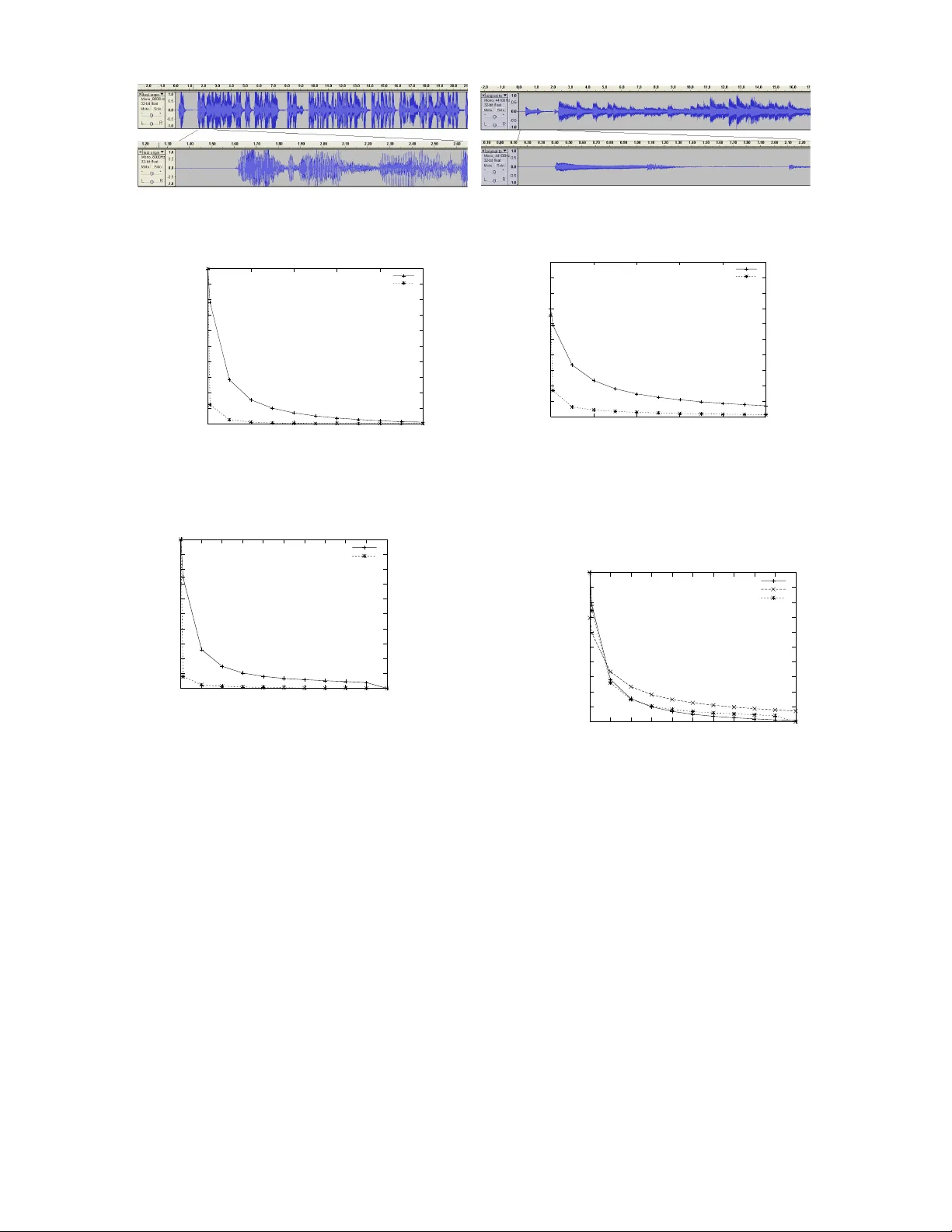
F ast and Quality-Guaranteed Data Streaming in Resour ce-Constrained Sensor Netw orks Emad Soroush Dept. of Computer Science Unive rsity of Victor ia Victoria, BC Canada V8W 3P6 soroush@csc.uvic.ca K ui W u Dept. of Computer Science Unive rsity of Victoria Victoria, BC Canada V8W 3P6 wkui@csc.uvic.ca Jian P ei School of Computing Science Simon F raser University Burnaby , BC Canada V5A 1S6 jpei@cs.sfu.ca ABSTRA CT In many emerg ing applications, data streams are monitored i n a network en vironment. Due to limited communication bandwidth and other resource constraints, a criti cal and practical demand is to online compress data streams continuously with quality guar- antee. Although many data compression and digital si gnal pro- cessing methods hav e been dev eloped to reduce data volume, their super-linear time and more-than-constan t space complexity pre- vents them from being applied directly on data streams, partic- ularly over resource-con strained sensor networks. In this paper , we tackle the p roblem of online quality guaran teed compression of data streams using fa st linear approximation (i.e., using line seg- ments to approximate a time series). T echnically , we address two versions of the problem which explore quality guarantees in dif- ferent forms. W e dev elop online algorithms with linear time com- plexity and constant cost in space. Our algorithms are optimal in the sense they generate the minimum number of segments that ap- proximate a ti me series with the required quality guarantee. T o meet the resource constraints in sensor networks, we also dev elop a fast algorithm which creates connecting segments with very sim- ple computation. The low cost nature of our methods leads to a unique edge on the applications of massiv e and fast streaming en- vironment, lo w band width netwo rks, an d hea vily constrained node s in computational power . W e i mplement and ev aluate our methods in the application of an acoustic wireless sensor network. Categories and Subject Descriptors C.3 [ Computer S ystems Organization ]: Special-Purpose and Ap plication-Based S ystems; G.1.2 [ Mathematics of Computing- Numerical Analysis ]: Approximation- Linear appr oximation General T erms Algorithms, Design, Performance Keyw ords W ireless Sensor Netw orks, Data Streaming, Linear Approximation 1. INTR ODUCTION In many emergin g applications, massiv e data streams are mon- itored in a network en vironment. For example, large sensor net- works are extensi vely used i n wildlife monitoring, road traffic mon- itoring, an d en vironment surv eillance. E ach sensor generates a data stream where new data entries (i.e., new readings) keep arriving in a continuous ma nner . In order to aggregate and an alyze the massive streaming data u nder monitoring, it is often required to transmit the data streams in the network. Due to often limited communication bandwidth and other resource constraints, online compressing data streams continuously with qua lity guarantee rises as a natural, crit- ical and practical demand in those applications. E X A M P L E 1 ( M OT I V A T I O N ). W e, the authors of this paper , are building an acoustic monitoring system using wireless sensor networks. Sensor nodes are deployed in a t arget area, while each node c ontains an acoustic sensor which samples sound signals con- tinuously . The sensor nodes are connected by a wireless network. The acoustic monitoring system has many applications. An ap- pealing scenario is to wards “smart conference hall. ” By analyzing the data collected from an acoustic monitoring system deployed in a large conference place, we can identify and locate speak ers as well as some of their activities. The information can be used to adjust the equipment such as the light system , the microphone sys- tem, the video monitoring sy stem, and the air conditioning system. Another potential application is bird surveillance in wildness. By analyzing the bird sound co llected using such a sensor n etwork, or- nithologists can study the distr ibution of birds and their behavior patterns. W ireless sensor nodes which inte grate sensors, processors, mem- ory and wireless transcei vers often are small and have only very limited computational powe r and communication bandwidth. For instance, the Chipcon radio chip in the broadly-used MICA2 motes [15] has the maximum transmission power of 27 mA and the max- imum bandwidth of 38 kbps. In our acoustic monitoring system, we use MICA2 motes. One technical cha llenge is t hat, altho ugh a sens or can sample th e acous- tic signa ls frequently , the acoustic data stream cannot be sent ou t in time due to the lo w bandwidth radio channel. S pecifically , in order to make the data analysis useful, we need to sample human voice with the normal sampling rate of 8 kHZ and 16 bits per sample. This sampling mode requires the bandwidth of 128 kbps for 1 chan - nel ( mono) voice, which greatly exceed s the maximum bandwidth of 38 kbps that an MICA2 mote can support.In addition, we can- not temporarily store a large number of samples since the memory size of MICA2 motes is only 512 kb . The only technical solution to the bottleneck is to online compress data streams continuous ly and send ou t the compresse d streams instead of the original streams through the network. Sending compressed streams can also reduce the po wer consumption of sensors on co mmunication, and thus ex - tend lifetime of sensors. In lar ge en vironmental surveillance sensor networks, rechar ging or re placing batteries of sensor nodes is often very dif ficult or ev en impossible after the sensors are deployed . Many data compression and digital signal processing methods hav e been de veloped t o reduce data volume, such as Fourier trans- form [17], discrete cosine transform [14], W avelets [2], l inear pre- dictiv e coding (L PC) [1 ], etc. Howe ver , those methods cannot be applied to data stream compression in sensor networks due to the high cost of those methods in time and space. Moreo ver , sensor nodes like MICA2 motes only have very l imited computational po wer . For example, only simple arit hmetic operations are sup- ported by T inyOS [3], the operating system for MICA2 motes. Al- though it i s possible to implement a mathematical module to cal- culate essential functions like sinusoid and exponential functions or use dedicated DS P chips for audio processing and compression, such complex modules are highly undesirable due to the l imited memory size and computational capacity of MICA2 motes as well as the extra ener gy cost of dedicated DSP chips. In this paper , we tackle the problem of online compression of data streams in the application context of sensor networks. Partic- ularly , we aim at the fast linear approximation methods (i .e., using line seg ments to approximate a time series) with quality guarantee. W e make the follo wing contributions. First, we model the piecewise linear approximation problem prop- erly for data streams. Different from the con ventional situations where t he whole time series to be compressed and the required compression rate can be specified, a data stream is potentially un- limited, and the distrib ution is often unpred ictable. W e pro pose the error-bou nded piece w ise linear approximation problem to tackle those cha llenges. Second, we p resent fast online solutions with lin- ear time comple xity and constant cost in space . Our algorithms are optimal in t he number of segments used to approximate a (poten- tially unlimited) time series. In other words, our algorithms create the minimum number of line segments even w ithout knowing the futur e incoming data . T o the best of our knowledg e, we are the first to successfully de vise al gorithms with such strong guarantees. Third, to add ress the computational challenges in sensor nod es, we de velop a nother online approximation algorithm th at is particularly tailored for tiny sen sor devices b y requiring only very simple com- putation. The low cost nature of our methods leads to a unique edge on t he applications of massiv e and fast streaming en viron- ment, low bandwidth network s, and heavily constrained nodes in computational po wer (e.g., tiny senso r nodes). Last, we implement and ev aluate our methods in the application of an acoustic wire- less sensor network. Our empirical ev aluation clearly shows that our methods are highly feasible for resource-constrained wireless sensor networks. The rest of the paper is organized as follows. In Section 2, we formulate and analyze the problem, and re view the related work. T wo online algorithms are dev eloped in Section 3, and their opti- mality is studied in Section 4. In Section 5, we design an online approximation al gorithm which is more economic in computation for tiny sensors. W e report our implementation and ev al uation of the proposed methods in an acoustic wireless sensor network in Section 6. T he paper is concluded in Section 7. 2. PR OBLEM DEFINITION AND RELA TED WORK In this section, we propose the error-bounded piecewise linear approximation problem for data streams. W e also revie w the related work. 2.1 Pr oblem Formulation Piecewise linear approximation (P LA) is an effecti ve method to compress a time series. A numeric data stream can be treated as a potentially unlimited time series. Thus, it is natural to explore whether we can compress a numeric data stream using the piece- wise linear approximation method. Let X = x 1 · · · x n be a time seri es o f n points, and x i (1 ≤ i ≤ time t o C’ C B’ B A’ A value Figure 1: Piecewise linear approximation. n ) be the va lue of the i -th point of X . A (line) se gment i s a tuple s = (( i, y i ) , ( j, y j )) where i < j and ( i, y i ) and ( j, y j ) are two endpoints. [ i, j ] is called the rang e of s . Giv en a time series X , PLA uses a set of line segmen ts as the approximation of t he time series. Figure 1 elaborates the general idea, where three line segmen ts, A A ′ , B B ′ , and C C ′ , are used to approximate a time series. A line segment s = (( i, y i ) , ( j, y j )) approximates the k -th point ( i ≤ k ≤ j ) of the ti me series by value ˜ x k = y i + k − i j − i ( y j − y i ) . The compression comes from that the number of line segme nts us ed for approximation can be much smaller than the number of points in the time series. In the figure, the time series has 18 points. three segmen ts are used to approximate the t ime series, and each seg- ments has 2 endpoints. Thus, the 3 line segments only need 6 points to represent. A compression ratio of 3 is achieve d. Generally , the endpoints in the segm ents are not necessarily positioned at some points in the time series (e.g., B , B ′ , and C ′ in the figure). Formally , a set of segments ˜ X = { s 1 , . . . , s m } is a piece wise linear approximation of X i f (1) s 1 , . . . , s m are segm ents; and (2) for each index i (1 ≤ i ≤ n ) , i i s either in the range of exactly one segment in ˜ X , or t here exist two segmen ts s, s ′ ∈ ˜ X such that s and s ′ share the same endpoint at index i . Clearly , using the segmen ts, for ev ery index i , ˜ X can giv e a value ˜ x i to approximate x i . PLA for stati c time series has been well studied (e.g., [5, 6, 8, 12]). Most of the pre vious stud ies address an optimization problem as follows. P RO B L E M 1 ( C O N V E N T I O NA L P L A P RO B L E M ). Given a time series X of n points and a number m < n , find a set o f m se gments as a piece wise linear appr oximation of X such that the appr oxima- tion err or is minimized. Unfortunately , solutions to the con ven tional PLA problem are not applicable to data streams. A data st ream is potentially unlim- ited. It is impossible to know in adv ance th e nu mber of points in t he stream or to specify the number of se gments to be u sed for approx - imation. T o t ackle the stream compression problem, in this paper, we turn to the err or-boun ded PLA pr oblem . P RO B L E M 2 ( E R RO R - B O U N D E D P L A P RO B L E M ). Given an err or measur ement function er r () such that er r ( X, ˜ X ) gives the err or that a P LA ˜ X appr oximates X . Let ǫ be a user-spec ified err or bound. ˜ X is called an ǫ -PLA of X if er r ( X , ˜ X ) ≤ ǫ . An ǫ -P LA ˜ X of X is optimal if | ˜ X | (i.e., the number of seg ments in ˜ X ) is minimized. W e propose two error measurem ent functions meaningful for data streams. First, the max-err function captures the maximal error between X and ˜ X at any index . T hat is, maxer r ( X , ˜ X ) = n max i =1 {| x i − ˜ x i |} W ith potentially unlimited streams, using the max-err function, we can mak e sure t he approximation quality is consistently boun ded at e very point. Second, the se g-err function checks the error introduced by each segmen t, and captures the maximal error . That i s, seg er r ( X , ˜ X ) = max s ∈ ˜ X { X i ∈ r ange ( s ) ( x i − ˜ x i ) 2 } Using the seg-err function, we can make sure that the err or intro- duced by ev ery segmen t is bounded. Using the two error measurement functions, we hav e two ver- sions of the error-bounde d P LA problem. P RO B L E M 3 ( P L A - P O I N T B O U N D P R O B L E M ). Given an err or- bound ǫ , the PLA-PointBound problem is to find an ǫ -PLA ˜ X such that maxer r ( X , ˜ X ) ≤ ǫ and | ˜ X | is minimized. P RO B L E M 4 ( P L A - S E G M E N T B O U N D P RO B L E M ). Given an err or-bou nd ǫ , the PLA- SegmentBou nd problem is to find an ǫ - PLA ˜ X such that seg er r ( X , ˜ X ) ≤ ǫ and | ˜ X | is minimized. 2.2 Related W ork Piecewise linear approximation (P LA) has been well in vestigated in [4, 7, 8, 12, 13, 16]. The idea behind PLA comes f rom the fact that a sequence of line segments can be used to represent the time series while preserving a low approximation error . Standard linear regression techniqu e is widely used in most existing piece wise lin- ear approximation algorithms to calculate a line segmen t approx- imating the original data with t he minimum mean squared error . Many of them [ 5, 6, 8, 12] target at solving the conv entional P LA problem and may not be applicable to streaming data. Despite the substantial research efforts in P LA techniques [5 , 6, 7, 11, 8, 12], existing solutions are not tailored for data streams over resource-constrained sensor n etworks. They either require com plex computation or hav e high cost in space. T o the best of our kno wl- edge, there has no implementation of these algorithms in realistic sensor de vice. In [9], the autho rs use PLA to estimate a time series. But the au- thors put unnecessary constraints on the algorithm, which requires the endpoints come from the original dataset. On the whole, t heir algorithm can run in O ( n 2 log n ) time complexity and takes O ( n ) space complexity . In [7], Keo gh et al. gi ve a comprehensiv e revie w on the existing techniques for segmenting time series. They categorize the solu- tions into three different groups, namely sliding wi ndo w methods, top-do wn methods, and bo ttom-up methods. They then take advan- tage of both sliding windo w and bottom-up methods and design a Sliding-W indow-And -Bottom-up (S W AB) algorithm. The SW AB algorithm uses a moving wind ow to constrain a time period i n con - sideration. In [11], an a mnesic function is introdu ced to gi ve weights to dif- ferent points in the time series. The PLA-SegmentBound problem is discussed in t he context of Unrestricted Wind ow with Absolute Amnesic (UAA) problem, but complete solutions to this problem are not provid ed in [11]. A solution t o the PLA-P ointBound prob lem is addressed i n [10] with a different definition of point error bound. The algorithm is claimed to be optimal, b ut the time com plexity is O ( n 3 ) where n is the number of points in t he time series. Moreover , no performance e valuation of the solution is presented in the paper . In summary , although the error-bounde d PLA problem has been in vestigated before, the problem has not been studied systemati- cally . No solutions applicable to data streams hav e b een de veloped, let alone solutions for resource-con strained sensor networks. 3. ONLINE ALGORITHMS In this section, w e de velop two online algorithms for the PL A- PointBound and the PLA-SegmentBound problems, respectiv ely . The two algorithms share the same frame work. 3.1 The Framework The frame work of our algorithms wo rks in a greed y mann er . When x 1 , the first point i n t he stream, arriv es, we store x 1 . When x 2 arriv es, we also store x 2 since x 1 and x 2 can be compressed by a segment exactly . When x 3 arriv es, we check whether x 3 can be compressed together with x 1 and x 2 by a line segment satisfying the error-bound requirement. If so, we store x 3 . Otherwise, we output a line segment compressing x 1 and x 2 , remove x 1 and x 2 from the main memory , and store x 3 . Generally , i magine we have a buf fer in main memory storing points x i , x i +1 , . . . , x j such t hat the points in the buf fer can be compressed by a line segmen t satisfying t he error-bound require- ment. When a new point x j +1 arriv es, we check whether x j +1 can be compressed together with x i , . . . , x j by a li ne segme nt sat- isfying the error-bound requirement. If so, we add x j +1 to the buf fer and move on to the next point. Otherwise, we output a seg- ment compressing x 1 , . . . , x j satisfying the error-bound require- ment, and remove them from the buf fer . x j +1 is then stored in the buf fer . Although the framew ork is simple, there are t wo criti cal issues that need to be solved carefully in order to make sure that the runtime of the algorithms is linear with respect t o the number of points in the streams, and the space si ze needed by the algorithms is bounded by a constant. First, ho w can we s tore the informa tion about the points we have seen but hav e not compressed? In the worst case, t here can be an unlimited number of such points (e.g., a times series where all points take the same value). Ho w can we summarize them using only constant size memory? Second, how can we determine whether a newly arriv ed point can be compressed together with the points already in the buf fer that hav e been seen but have not been compressed? Rev isiting t hose points one by one leads to the runtime quadratic with respect to the number of such points. As exp lained before, there can be an unlimited number of such points. T he ove rall time complexity is quadratic if those points are rev isited one by one. Our ce ntral idea t o tackle the abov e two challenges is the follow- ing. Instead o f storing the points ex plicitly , we monitor the rang e o f all possible line segments that can be used to compress the points that have been seen but have not bee n compress ed in a concise way . When a new point arriv es, w e can check whether the point can be compressed using some l ine segment in t he range. If so, i t means that the ne w point can be compressed together wi th the points ac- cumulated. W e only need to adjust the range of t he possible line segmen ts t o make sure the ne w point is also compressed. If not, it means t hat the new point cannot be compressed together with the points accumulated. A segment sho uld be output. 3.2 Solving the PLA-P ointBound Problem A segment s = (( i, y i ) , ( j, y j )) can also be represented by the tim e i j ... x i x j x i - ε x i + ε y i x j + ε x j + ε Sl o pe: m 1 = (x j + ε -y i )/(j-i ) Sl o pe: m 2 = (x j - ε -y i )/(j-i ) Figure 2: Ranges of possibl e line segments. y i m (S l ope) x i + ε x i - ε m 1 = (x j + ε -y i )/(j-i ) m 2 = (x j - ε - y i )/(j-i ) poly(i,j) Figure 3: Polygon poly ( i, j ) . left endpoint ( i, y i ) , the slope m = y j − y i j − i , and the index of the right endpoint j . For two points x i and x j in a data stream, if a line segment s = (( i, y i ) , ( j, y j )) with slope m = y j − y i j − i can approximate x i and x j , i.e., | x i − ˜ x i | ≤ ǫ and | x j − ˜ x j | ≤ ǫ where ǫ is the error-boun d, s must satisfy the following four con ditions. ( x i − ǫ ) ≤ y i ≤ ( x i + ǫ ) (1) m 1 = ( x j + ǫ ) − y i j − i (2) m 2 = ( x j − ǫ ) − y i j − i (3) m 2 ≤ m ≤ m 1 (4) Figure 2 illustrates the conditions and their relations. Particularly , m 1 and m 2 are the slopes of the two lines sho wn in the figure. Since the li ne segme nts are determined by the value of the left endpoint y i and slope m , we examine t he distribution of points ( y i , m ) that satisfy E quations 1 to 4. As illustrated in Figure 3, the possible line segments form a polygon pol y ( i, j ) . W e hav e the follo wing i mportant result. L E M M A 1 ( P L A - P O I N T B O U N D ) . A line seg ment of left end- point y i and slop e m can appr oximate points x i , . . . , x j with max- err at most ǫ if and only if ( y i , m ) is in polygon pol y ( i, i + 1) ∩ poly ( i, i + 2) ∩ · · · ∩ p oly ( i, j ) . Proof . T he necessity follows with the definition of poly ( i, j ) . For any line segment s 6∈ pol y ( i, i + 1) ∩ poly ( i, i + 2) ∩ · · ·∩ pol y ( i, j ) , there exists a n index k ( i ≤ k ≤ j ) such that s 6∈ poly ( i, k ) , i.e., s cannot approximate either x i or x k . W e prov e the sufficiency by contradiction. Suppose a segment s ∈ pol y ( i, i + 1) ∩ poly ( i, i + 2) ∩ · · · ∩ pol y ( i, j ) but s cannot approximate x k ( i ≤ k ≤ j ) . T wo situations may arise. First, k = i . Then, s 6∈ poly ( i, i + 1) since | x i − y i | > ǫ where y i is Input: a data stream X = x 1 , x 2 , . . . and err or-bou nd ǫ ; Output: a list of line seg ments ˜ X approximating X such that maxer r ( X , ˜ X )) ≤ ǫ ; Method: 1: P = pol y (1 , 2) ; i = 1 ; j = 3 ; 2: WHILE (1) DO { 3: P ′ = P ∩ poly ( i, j ) ; 4: IF P ′ 6 = ∅ THEN P = P ′ , j = j + 1 ; 5: ELSE { 6: randomly choose a point ( y , m ) i n P ; /*any point in P meets the point err or bound*/ 7: output a line segme nt (( i, y ) , ( j − 1 , y + ( j − 1 − i ) ∗ m )) ; 8: P = pol y ( j, j + 1) ; i = j ; j = j + 2 ; } } Figure 4: PointBound, an online algorithm fo r the PLA- PointBound pr oblem. the value of s on index i . Second, k 6 = i . T hen, s 6∈ pol y ( i, k ) . In both cases, we hav e contradictions. Using Lemma 1, we hav e algorithm PointBound, an online algo- rithm as sho wn in Figure 4. W e maintain the i ntersection of poly- gons poly ( i, i + 1) , . . . , pol y ( i, j ) , where x i is the fi rst point t hat has not been compressed yet in the data stream, and x j is the last point arriv ed such that poly ( i, i + 1) ∩ . . . ∩ pol y ( i, j ) 6 = ∅ . When a new point x j +1 arriv es, we compute poly ( i, j + 1) and poly ( i, i + 1) ∩ . . . ∩ p oly ( i, j ) ∩ poly ( i, j + 1) . If it is ∅ , then a line segment s is randomly chosen to approximate x i , . . . , x j such that ( y i , m ) is in poly ( i, i + 1) ∩ . . . ∩ poly ( i, j ) , where y i is the v alue of s on index i , and m is the slope of s . s is output, and the intersection of polygon is remov ed. x j +1 and x j +2 are used to generate a ne w polygon p oly ( j + 1 , j + 2) . If poly ( i, i + 1) ∩ . . . ∩ pol y ( i, j ) ∩ poly ( i, j + 1) 6 = ∅ , then the intersection is k ept, and t he algorithm moves on to the ne xt po int in the stream. For any i and j , pol y ( i, j ) i s a parallelogram where there are two edges parallel to the slope axis. It is easy to show that fo r any i and j , ∩ j k = i poly ( i, k ) is a con vex p olygon. In the worst case, t he edges of the intersection of parallelograms could be up to 2( j − i + 1) , i.e., twice the number of parallelograms intersected. A straightfor- ward method keepin g all edges of the intersection area still has the quadratic time complexity and linear space complexity , which are not applicable to data streams. Fortunately , we do not need to record all edges of t he intersection polygon. Instead, we need to r ecor d on ly up to 4 edges to d etermine whether a new point can be compr essed tog ether with the points seen but no t compr essed. Using E quations 1 to 4, it is easy to see that each parallelogram has two properties: (1) Each parallelogram has t wo vertical edges and two sloping edges wi th a negati ve slope v alue, as shown in Figure 3. The range of y i is t he same for all parallelograms (i.e., x i − ǫ ≤ y i ≤ x i + ǫ ). (2) For j 2 > j 1 > i , the absolute slope v alue of the two sloping edges in poly ( i, j 2 ) is strictly smaller than the absolute slope v alue of the two sloping edges in pol y ( i, j 1 ) . Let us focus on the intersection points of the upper sloping edge of parallelograms. The case for the lowe r sloping edges can be analyzed similarly . The situations are illustrated in Figure 5. Suppose that the fi rst parallelogram gi ves t he upper sloping edge AB with slope v alue Figure 5: Usi ng up to 4 edges to r epresent the in tersection p oly- gon. m AB as in Figure 5(a). When a ne w data point arrive s, a new parallelogram is formed. In the worst case, the upper sloping edge of the parallelogram C D cuts AB into t wo parts. Let E be the intersection point between AB and C D , as shown in Figure 5(b). By the second property , we hav e | m C D | < | m AB | . Moreov er , the upper sloping edge F G of any future parallelogram cannot cut both C E and E B due to the smaller absolute slope value of F G than m C D . In other words, if a future parallelogram intersects wi th the current intersection polygo n, the upp er sloping edge of the par- allelogram can only cut either C E , E B or the right vertical edge. Instead of keeping C E and E B , we can keep l ine segment C B . Then, a future parallelogram intersects with the current intersec- tion polygon if and only if it cuts C B . Generally , we only nee d to keep the line segment con necting the left-most upper corner and the right-most upper corner for the up- per sloping edges. Simil arly , we only need to keep the line segmen t connecting the left-most lower corner and the right-most lower cor- ner for the lowe r sloping edges. In addition to this two line segmen ts, we need to keep the two vertical edges in the intersection poly gon. T he reason is tha t the in- tersection of two parallelograms may shrink the range of the inter- section, as illustrated in Figure 5(c), where parallelogram AB C D intersects with parallelogram E F GH . The left vertical edge is shrunk into a point I ri ght to the original edg e. In summary , we need to r ecord only up to 4 edges to determine whether a new point can be compressed together with the points seen but not compressed. This immediately leads to the following result. T H E O R E M 1 ( C O M P L E X I T Y – P O I N T B O U N D ). The algorithm P ointBound for the PLA -P ointBound pr oblem has the time comple xity O ( n ) and the space complexity O (1) , wher e n is the number of points in a time series to be compr essed. Since algorithm PointBound only looks ahead for one point in the data stream to output a li ne segm ent whene ver necessary in the piece wise linear approximation, it is an online algorithm and can be applied on data streams. 3.3 Solving the PLA-SegmentB ound P r oblem W e first p resent th e f ollo wing useful observation, to which a sim- ilar result has been reported in [12] without proof. L E M M A 2. Suppose that a line se gment s appr oximates a fr ag- ment X of n points x 1 , . . . , x n in a time series. Then, s minimi zes seg er r ( s, X ) if the slope of s is m = ( P n i =1 ix i ) − 1 n P n i =1 i P n i =1 x i ( P n i =1 i 2 ) − 1 n ( P n i =1 i ) 2 (5) and the left endpoint of s has value m + P n i =1 ( x i − i · m ) n Input: a data stream X = x 1 , x 2 , . . . and err or-bou nd ǫ ; Output: a list of line seg ments ˜ X approximating X such that maxer r ( X , ˜ X )) ≤ ǫ ; Method: 1: i = 1 ; j = 3 2: s = the line segment ((1 , x 1 ) , (2 , x 2 )) ; 3: WHILE (1) DO { 4: s ′ = the line segmen t identified in L emma 2 to compress x i , . . . , x j ; 5: IF seg err ( s ′ , x i · · · x j ) ≤ ǫ THEN 6: s = s ′ ; j = j + 1 ; 7: ELSE { 8: output s ; 9: i = j ; j = j + 2 ; 10: s = the line segment (( i, x i ) , ( i + 1 , x i +1 )) ; } } Figure 6: S egmentBound, an online algorithm for the PLA- SegmentBound problem. Proof . Consider a li ne segment s approximating fragment X . Let the left end point of s be (1 , y 1 ) and the slope be m . For each p oint x i (1 ≤ i ≤ n ) , the error is | x i − ˜ x i | = | x i − y 1 − m ( i − 1) | . Thus, seg er r = n X i =1 ( x i − y 1 − m ( i − 1)) 2 (6) Clearly , when y 1 = m + P n i =1 ( x i − i · m ) n , seg err reaches the mini- mum v alue seg er r = n X i =1 x 2 i + m 2 n X i =1 i 2 − 2 m n X i =1 x i i − ( P n i =1 ( x i − i ∗ m )) 2 n (7) From Equation (7), when m = ( P n i =1 ix i ) − 1 n P n i =1 i P n i =1 x i ( P n i =1 i 2 ) − 1 n ( P n i =1 i ) 2 seg er r i s minimized. Lemma 2 leads to algorithm SegmentBoun d, an online al gorithm for the PL A-SegmentBoun d problem as shown in Figure 6. S up- pose x 1 , . . . , x n are the points that hav e not been compressed yet. When a ne w po int x n +1 arriv es, we check wh ether the line se gment identified by Lemma 2 can achie ve the segment error bound. If so, then x n +1 is added into the buf fer , and the algorithm moves on to the ne xt point in the stream. Otherwise, the line segment suggested by L emma 2 for points x 1 , . . . , x n is output, and x 1 , . . . , x n are considered compressed . x i + n is added into the bu ffer . When a ne w data point x n +1 arriv es, the left endpoin t and t he slope of the line segment suggested by Lemma 2 can be calculated quickly . T echnically , Equations (5) and (7) indica te that we need to calculate P n +1 i =1 i , P n +1 i =1 x i , P n +1 i =1 x i i , P n +1 i =1 x 2 i , and P n +1 i =1 i 2 . Since we already have P n i =1 i , P n i =1 x i , P n i =1 x i i , P n i =1 x 2 i , and P n i =1 i 2 , the addition of the new point only incurs a constant cost to update the values of m and the left endpoint . T his leads to the follo wing result. T H E O R E M 2 ( C O M P L E X I T Y – S E G M E N T B O U N D ). The algorithm Se gmentBound for the PL A-Se gmentBound pr oblem has the time comp lexity O ( n ) and sp ace complex ity O (1) , wher e n is the number of points in a time series to be compr essed. 4. OPTIMALITY T H E O R E M 3 ( P L A - P O I N T B O U N D Q U A L I T Y ). The P ointBound algorithm in Section 3.2 pro duces a minimum num- ber of se gments to compr ess a time series. Proof . For a time series X = x 1 , . . . , x n , let l = min {| ˜ X |} , where ˜ X is an ǫ -PLA approximating X (i.e., m axer r ( X , ˜ X ) ≤ ǫ ). W e conduct an i nduction on l to show that algorithm PointBound outputs an ǫ -PLA of l line segm ents. (Base case) Consider l = 1 , i.e., there exists a line segmen t that approximates the whole ti me series. According to Lemma 1, poly (1 , 2) ∩ · · · ∩ pol y (1 , n ) 6 = ∅ . T hus, algorithm PointBound finds a line segment s approximating x 1 , . . . , x n and maxer r ( s , X ) ≤ ǫ . (Induction) Assume that, when l ≤ k , algorithm PointBound finds an ǫ -PLA ˜ X of l line segments to approximate X . Now , let us consider the case of l = ( k + 1) , i.e., there exists an optimal ǫ -PLA ˜ Y = { s 1 , . . . , s k +1 } that approximates X . Suppose that s 1 approximates x 1 , . . . , x m . Let us assu me that s ′ 1 output by algorithm PointBound app roximates points x 1 , . . . , x m ′ . Due to Lemma 1, poly (1 , 2) ∩ · · · ∩ poly (1 , m ) 6 = ∅ . Thus, s ′ 1 must approximate x 1 , . . . , x m with the quality guarantee, i.e., maxer r ( s ′ 1 , x 1 · · · x m ) ≤ ǫ . In other words, m ′ ≥ m . If m = m ′ , then points x m +1 , . . . , x n in X can be approximated by an ǫ -PLA of ( l − 1) = k line segments. According to the assumption, algorithm PointBound finds an ǫ -PLA of ( l − 1) line segmen ts approximating x m +1 , . . . , x n . Suppose that m ′ > m . Si nce x m +1 , . . . , x n can be approx- imated by an ǫ -PLA of ( l − 1) line seg ments, a proper subset x m ′ +1 , . . . , x n must also be app roximated by an ǫ -PLA of at most ( l − 1) = k line segmen ts. W e only need to drop t he segments approximating x m +1 , . . . , x m ′ . According to the assumption, al- gorithm PointBound finds an ǫ -PLA of the minimum number of line segments to approximate points x m ′ +1 , . . . , x n . In summary , algorithm PointBound finds an ǫ -P LA of l = ( k + 1) line segments approximating X . Similarly , we can also show the optimality of the SegmentBound algorithm. T H E O R E M 4 ( P L A - S E G M E N T B O U N D Q UA L I T Y ). The Seg mentBound algorithm in Section 3.3 pro duces a minimum number of se gments to compr ess a tim e series. Although the number of line segments used to approximate a time series is a good measure on the compression quality , it i s not directly translated to compression ratio. For examp le, in our methods, the endpo ints of segmen ts are not constrained. Thus, two points are needed to represent a segment. On the other hand, a PLA using connecting segmen ts (i. e., two consecutiv e segments share the same endpoint) may use more segments but achiev e a better co mpression ratio since only one point is needed to represent a segmen t except for the first se gment. T H E O R E M 5 ( C O M P R E S S I O N FA C T O R ). Algorithms P ointBound and Se gmentBound have an appr oximation factor of 2 to the optimum compr ession factor that an ǫ -P LA can achie ve. Proof . W e only show the case f or t he PointBound algorithm. The same argument applies to the Seg mentBound algorithm. x i x j x k   tim e i j ... ... k x i x j x k   tim e i j ... ... k  x j ' (a) (b) Figure 7: An example of zoning angle For an y time series X of m points, suppose that the PointBound algorithm app roximates X using n line se gments. Then, according to Theorem 3, any PLA cannot have less t han n line segme nts. T o represent n line seg ments, at least ( n + 1) points are nee ded. Thus, the optimum compression ratio using PLA is at most α opt = m n +1 . The line segmen ts generated by t he PointBound algorithm may not be connecting. T hus, at most 2 n points are needed to represent the n line se gments. The worst case co mpression ratio of the Point- Bound algorithm is α P ointB ound = m 2 n . Cl early , α opt α P ointB ound = 2 n n +1 < 2 . 5. PLAZA FOR TINY SENSORS Although algorithm PointBound is optimal for the PL A-PointBound problem, it sti ll may be too computation intensiv e for tiny , resource- constrained sensors due to two reasons. First, algorithm P ointBound may generate non-connecting seg- ments such that each segment requires the t ransmission of two end- points. As analyzed before, connecting line segmen ts reduce the data transmission volume since each segme nt (excep t the first one) requires the transmission of only one endpoint. S econd, algorithm PointBound has to calculate intersection of parallelograms. The computation may be too heavy for tiny , resource-constrained sen- sor nodes. In this section, we d esign a simple, fast online algorithm PLAZA (P iece wise Linear A pproximation wi th Zoning Angle) for the P LA- PointBound p roblem. PL AZA generates co nnecting line seg ments. Although PLAZA is not optimal in the number of line segments used f or approximation, it is l ight in comp utation and very effecti ve in compression ratio, as will be verified by our e xperiments. 5.1 PLAZA PLAZA builds on the concept of zoning angle. Giv en an er- ror bound ǫ and two points ( i, x i ) and ( k , x k ) ( i < k ), the zon- ing angle from ( i, x i ) to ( k , x k ) , denoted by θ ǫ ( i,k ) , is defined as the angle that has ( i, x i ) as the endpoint, (( i, x i ) , ( k , x k )) as the bisector , and has a de gree of 2 arctan ǫ | x i x k | , where | x i x k | = p ( k − i ) 2 + ( x k − x i ) 2 . Figure 7(a) sho ws an e xample of zoning ang le θ ǫ ( i,k ) . The zo ning angle defines a zone to include an y potential line segmen ts that can be used to compress x i and x k . W e observe the follo wing important results. Their proof is t riv al and is omitted due to space limit. L E M M A 3. F or thr ee points x i , x k , x j ( i < k < j ) in a ti me series, the line se gment (( i, x i ) , ( j, x j )) appr oximates x k with er- r or up to ǫ if and only if the line se gment (( i, x i ) , ( j, x j )) falls in the zoning angle θ ǫ ( i,k ) . L E M M A 4. F or thr ee points x i , x k , x j ( i < k < j ) in a time se- ries, if zoning angle θ ǫ ( i,j ) has no over lap with zoning angle θ ǫ ( i,k ) , Input: a data stream X = x 1 , x 2 , . . . and err or-bou nd ǫ ; Output: an ǫ -PLA ˜ X of a list of connecting line segmen ts, i. e., maxer r ( X , ˜ X )) ≤ ǫ ; Method: 1: i = 1 ; ang l e = θ ǫ (1 , 2) ; 2: s = line segment ((1 , x 1 ) , (2 , x 2 )) ; j = 3 ; 3: WHILE (1) DO { 4: ang l e = ang l e ∩ θ ǫ ( i,j ) ; 5: IF ang le 6 = 0 THEN { 6: IF segment (( i, x i ) , ( j, x j )) falls in ang le 7: THEN s = line segment (( i, x i ) , ( j, x j )) ; 8: ELSE { 9: x ′ j = the v alue of the bisector line of ang l e at inde x j as shown in Figure 7(b); 10: s = the line segment (( i, x i ) , ( j, x ′ j )) ; 11: x j = x ′ j ; 12: } 13: j = j + 1 ; 14: } 15: ELSE { 16: output s ; 17: i = j − 1 ; x i = x j − 1 ; j = j + 1 ; 18: ang l e = θ ǫ ( i,i +1) ; 19: s = line segment (( i, x i ) , ( i + 1 , x i +1 )) ; 20: } 21: } Figure 8: Algorithm PLAZA. ther e does not e xist a line se gment s with ( i, x i ) as th e left endpoint such that maxer r ( s, x i · · · x k · · · x j ) ≤ ǫ . Algorithm PLAZA works as follows. St arting from a point x i , Lemma 3 i s used to check if there i s a line segmen t approximating points between i ndex es i and j ( i < j ) . Moreover , Lemma 4 is used to check if searching further in the time series is futile. The pseudoco de of PLAZA is sho wn in Figure 8. Algorithm PLAZA scans each po int in a data stream only once and stores on ly the zon- ing angle and the current approximating segment in main memory , the a lgorithm clearly has linear time comp lexity an d constant space complex ity . 5.2 Benc hmarking PLAZA PLAZA creates connecting line segments. Only transmission of one point is needed for each l ine segmen t except for the fi rst line segmen t. This feature distinguishes PL AZA f rom algorithms Point- Bound and SegmentBound. What is the optimal compression that can be achiev ed by an ǫ -PLA consisting of only connecting line segmen ts? The idea behind the optimal PLAZ A benchmark algorithm is similar to that of algorithm P ointBound. T he main differen ce is that, unlike the P ointBound algorithm, we do n ot start the ne w seg- ment wi th t he initi al condition x i − ǫ ≤ y i ≤ x i + ǫ , where y i is the v alue of the left endpoint of the ne w segment. Instead we set a smaller range on y i to guarantee the connecti vity of two consec- utiv e segments. Specifically , to decide the range of y i , we use the last non-empty polygon intersection in the prev ious point. W e find the optimal solution by a thorough search. Starting from x 1 , we try all values of j such that x 1 , . . . , x j can be ap- proximated by a line segment with maximal error ǫ . F or each such a subset x 1 , . . . , x j , we compute t he intersection of paral- lelograms p ol y (1 , 2) ∩ · · · ∩ p oly (1 , j ) , and try to find a line seg- ment with left endpoint ( j, y j ) that can approximate some points x j +1 , . . . , x i where j + 1 < i and y j is in the r ange confined by poly (1 , 2) ∩ · · · ∩ pol y (1 , j ) . By doing so, the first and t he sec- ond li ne segments are connected. W e conduct a depth-first search to find an ǫ -PLA consisting of the minimum n umber of connecting line segments. Limit ed by sp ace, we omit the details here. The optimal PLAZA benchmark is an of fline algorithm: it as- sumes the time series is given and can be scanned multiple times. Its complexity is far abov e linear due to the t horough search. T his algorithm is obviou sly not suitable for online compression of data streams. It is for comparison purpose only . 6. EXPERIMENT AL EV ALU A TION In t his section, we ev aluate the performance of our online al go- rithms by si mulation in Matlab and by real implementation with MICA2 motes [15]. 6.1 Experimen tal Setting W e generated t wo audio fi les for t est. The first file includes hu- man voice with t he sampling rate of 8 khz in mono channel. The second file includes piano music with the sampling rate of 44 khz in mono channel. Each fi le i ncludes 1 , 000 , 000 samples, and the size o f each sample is 16 bits. F igures 9 a nd 10 show the w ave form of t he human voice data and the wav eform of the piano music, re- specti vely . It can be seen that the music data is much “smoother" than the hum an voice data. W e use the files to test the performance of our online al gorithms i n bandwidth saving . W e measure t wo metrics: 1. Sample r eduction ratio (i n verted compr ession ratio) . It is defined as the total number of points to represent the ǫ -PL A di vided by the total number of points in t he original ti me series. 2. Dist ortion . I t is defined as P n i =1 ( x i − ˜ x i ) 2 n , where n is the total number of points in the time series, x i is the original v alue, and ˜ x i is the approximated v alue of x i . In si mulation, we apply the online algorithms on t he audio files and measure the sample reduction rati o. Simulation results are re- ported i n Section 6.2 and Secti on 6.3. In the test using MICA2 motes, the original audio files are played on a desktop computer and are monitored and transmitted with a MICA2 mote ov er wire- less channel to a laptop computer . More details are provided in Section 6.4. 6.2 Results on Quality 6.2.1 Results on Sample Reduction Ratio Figures 11 and 12 sho w the results of algorithms PointBound and SegmentBoun d, respecti vely , with r espect to v arious error bound v alues. As shown in the figures, we can obtain a higher bandwidth saving on piano music than on human voice . By replaying the audio files recov ered from the samples by our algorithms, we per- cei ve th at the human voice recov ered from the samples by our algo- rithms i s fully recogn izable with the se gment error bound up to 0 . 4 , or with the point error bound up to 0 . 2 . The quality of recov ered piano music is acceptable to us with the se gment error bound up to 0 . 2 , or with the point error bound up to 0 . 1 . Figures 11 and 12 clearly demonstrate significant bandwidth sav- ing. With the online algorithms, we only need to transmit around 5% of the original sample size for piano music and around 20% of Figure 9: The wav ef orm of the human voice d ata ( the lower part is in a smaller time scale). Figure 10: The wav eform of th e piano music d ata (the lower part is in a smaller time scale). 0 0.1 0.2 0.3 0.4 0.5 0.6 0.7 0.8 0.9 1 0 0.2 0.4 0.6 0.8 1 sample reduction ratio error bound Online PointBound Algorithm on human voice Online PointBound Algorithm on piano music Figure 11: The sample reduction ratio of PointBound. 0 0.1 0.2 0.3 0.4 0.5 0.6 0.7 0.8 0.9 1 0 0.2 0.4 0.6 0.8 1 sample reduction ratio error bound Online SegmentBound Algorithm on human voice Online SegmentBound Algorithm on piano music Figure 12: The sample reduction ratio of Segment- Bound. 0 0.1 0.2 0.3 0.4 0.5 0.6 0.7 0.8 0.9 1 0 0.1 0.2 0.3 0.4 0.5 0.6 0.7 0.8 0.9 1 sample reduction ratio error bound PLAZA human voice PLAZA piano music Figure 13: The sample reduction ratio of PLAZA . the original sample size for human voice. As such, both so und files can be transmitted with the current sensor nodes. Figure 1 3 sho ws th e sample reduction ratio of algorithm PLAZ A with respect to various point error bounds. W e can observe the similar phenomenon as in Fi gures 11 and 12. With PLAZA, we percei ve that the recovered human voice is f ully recognizable with the (point) error bound u p to 0 . 2 , and the quality of recov ered pian o music is acceptable to us with the (point) error bound up t o 0 . 1 . From Fi gure 13, the abo ve qualiti es correspond to the bandwidth reduction of nearly 3% of the original data size for piano music and about 15% of the original data size for human voice. One interesti ng phenomeno n is t hat the S egmen tBound algo- rithm can reduce sample transmission volume ev en if the error bound is set to zero, as sho wn in Figure 12. This is because in the audio fi les, there are some silent periods where the sample values are close t o zeros. The S egmen tBound algorithm finds a line seg- ment to approximate those situations. This nice feature, howe ver , does not exist in the algorithms for the P LA-PointBound problem. If the error bound is zero, the initial polygon is empty in the Point- Bound a lgorithm, and the degree of the initial feasible angle is zero in PLAZA, resulting in no sample reduction. 0 0.1 0.2 0.3 0.4 0.5 0.6 0.7 0.8 0.9 1 0 0.1 0.2 0.3 0.4 0.5 0.6 0.7 0.8 0.9 1 sample reduction ratio error bound Online PointBound Algorithm Online SegmentBound Algorithm PLAZA Figure 14: Comparison of the th ree algorithms on the human voice data set. Figure 14 compares algorithms PLAZA, PointBound, and Seg- mentBound on the human voice data set. The gap between algo- rithms PLAZA and PointBound i s very small when the error bo und is less than 0 . 5 . Algorithm PointBound leads to more samples than algorithm PLAZA when the error bound is less than 0 . 3 . The gap between algorithm S egmen tBound and the two algorithms for the PLA-PoinBound problem comes from the f act that, using the same error bound value, the PLA-SegmentBound problem puts a tighter error constraint than the PLA-PointBound problem. W e observe the similar performance comparison of the three algorithms on the piano data set, but omit the figures here du e to space limit. 6.2.2 Results on Distortion In Figures 15 and 16, we quantitati vely sho w the distortion of our algorithms on the human voice data set and the piano music data set, respecti vely . The ov erall distortion on human voice is larger tha n t hat on pian o music due to the “s moother" waveform in the music data set. With the same error bound, algorithm PLAZA 0 0.1 0.2 0.3 0.4 0 0.1 0.2 0.3 0.4 0.5 0.6 0.7 0.8 0.9 1 distortion error bound Online PointBound Algorithm Online SegmentBound Algorithm PLAZA Figure 15: The distortion on the human voice dataset. 0 0.1 0.2 0.3 0 0.1 0.2 0.3 0.4 0.5 0.6 0.7 0.8 0.9 1 distortion error bound Online PointBound Algorithm Online SegmentBound Algorithm PLAZA Figure 16: The distortion on the piano music voice dataset. has the largest distortion . Algorithm PointBound is the ne xt. Algo- rithm SegmentBou nd has the smallest distortion because the same error bound on t he P LA-SegmentBound problem and the PL A- PointBound problem poses a t ighter error constraint on the PL A- SegmentBoun d problem. T he smaller distortion, howe ver , comes with the cost of lower ban dwidth saving as analyzed before. 6.3 Benc hmarking PLAZA W e test t he performance of P LAZA comparing t o the optimal solution of its kind (i.e., using connecting line segments to t ackle the P LA-PointBound problem). Due to the high complex ity of the PLAZA Benchmark method, the audio files are too big to obtain the optimal results wit hin reasonable time. W e have to use a small portion of the audio files for this test. Interestingly , the PLAZA method and the optimal PL AZA bench- mark algorithm generate very similar PLA line segments. Audio files are usually filled wi th short silent periods wh ere sa mple v alues are close to 0 . Thus, algorithm P LAZA can obtain line segments very similar to t hose computed by the benchmark algorithm. W e omit the detailed figures due to space limit. 6.4 Results on Real Sensors W e implemented our online algorithms using MICA2 motes [15] from Crossbo w T echnology Inc. The test bed i s il- lustrated in Figure 17. A MICA2 mote includes a radio/processor board an d a se nsor board. The radio/proc essor board u ses 900 Mhz radio. T he sensor board includes a microphon e that can be used for sampling sound. The interface of the base stati on i s based on RS232. It acts as a gateway to connect the laptop and t he radio wireless sensor network. The original audio fil es are played on a desktop computer , monitored by a MICA2 mote, and transmitted ov er wi reless chann el from the MICA2 mote to the base station. The results about the sample reduction ratio on the real sensor test bed are close t o the simulation results using Matlab . But the audio quality obtained u sing the real test bed is w orse than that ob - tained in the Matlab simulation. The deterioration in audio quality is caused by the major restr iction of T inyOS [3], the current oper- ating system in MICA2 motes. The OS does not support multi ple threads and t hus it cannot perform radio transmission and sound sampling concurrently . Due to this limit, when we transmit data to the base station, the sensor board stops sampling and the sound during this period is missed, resulting in small silent gaps in the recov ered audio. Nev ertheless, we can sti ll recognize the human speech and the piano music. The same task can be carried out with the most recent, more adv anced sensor de vice, MICAz from the same company . W ith Figure 17: The test bed usin g r eal sensors. a higher price, MICAz sensors support up t o 250 Kbps wi reless transmission. This task, ho wev er , has neve r bee n fulfilled with lo w- end devices li ke MICA2. T o t his end, we break the l imit of scarce radio ban dwidth and carry out a task that is hard to achie ve without our fast online compression methods. 6.5 Evaluation in Other A pplications Although we only implemented the online algorithms in an acous- tic sensor monitoring system, our algorithms are actually applica- ble to many other application domains such as electrocardiogram (ECG) monitoring for patients. W e test our algorithm on an ECG data set The maximum value on the data set is 2 , 490 and the min- imum value is − 8 , 190 . W e test our online al gorithms wi th error bound vary ing fr om 1 to 100 . 0 0.1 0.2 0.3 0.4 0.5 0.6 0.7 0.8 0.9 1 0 5 10 15 20 25 30 35 40 45 50 55 60 65 70 75 80 85 90 95 100 sample reduction ratio error bound PLAZA online PointBound Algorithm online SegmentBound Algorithm Figure 18: Results on an ECG data set. Figure 18 compares the sample reduction rati o of algorithms PLAZA, P ointBound, and SegmentBound on the ECG data set. The performance of algorithms PLAZ A and PointBound is very similar . When the err or bound is set to over 35 , both algorithms can compress the data up to 10% of t he original si ze. The gap between algorithms Segmen tBound and PointBound comes fr om the fact that, using the same error bound, the PL A-SegmentBoun d problem and the PLA-P ointBound prob lem put a tighter error con- straint on the PLA-SegmentBound problem. 7. CONCLUSION In this paper , we tackle the problem of online compression of data streams in the resource-constrained network en vironment, where the traditional data compression techniques cannot apply . Particu- larly , we aim at fast piecewise linear approximation (P LA) meth- ods with quality guarantee. W e study two version s of the problem which explore quality guarantees in different forms. For the error bounded P LA problem, we design fast online algorithms running i n linear time complexity and requiring a constant space cost. The o n- line algorithms are also optimal in terms of the number of generated segmen ts. T o meet the needs from ti ny , resource-con strained sen- sors, we dev elop ano ther online algorithm that inv olves very si mple computation and generates connecting line segments. Our si mula- tion results and t he test using a real sensor test bed demonstrate that o ur fast online linear approximation methods are v ery ef fectiv e for data stream compression and transmission ov er low bandwidth networks with nodes heav ily constrained in computational power . Equipped with the insights gained i n this study , we see a lot of application opportunities for our methods. Meanwhile, there are also some interesting open questions for future work. For e xample, an interesting question is to design an online algorithm that can compute an ǫ -P LA consisting of connecting line segments that has an approximation factor to the optimum. Acknowledgeme nt This research was supported by Natural Sciences and Engineering Research Council of Canada (NSERC), Canada Found ation for In- nov ation (CFI), and the British Co lumbia Kno wledge De velop ment Fund (BCKDF). W e also thank Dr . E. Ke ogh for his informative comments and for providing the ECG dataset. 8. REFERENCES [1] B. S. Atal and L. S. Hanauer . Speech analysis and synthesis by linear predict ion of the speech wave . Jou rnal of the A coustic al Society of America , 50:637–655, 1971. [2] K.P . Chan and A. W . Fu. Efficie nt time series matching by wav elets. In ICDE ’99: Pr oceeding s of the 15th International Conferen ce on Data Engineering , pages 126–133, W ashington, DC, USA, 1999. IEEE Computer Society . [3] D.E. Cull, J. Hill, P . Bounadonna, R. Szewc zyk, and A. W oo. A netw ork-centric approach to embedded software for tiny de vices. In Pr oceedings of F irst Internati onal W orkshop on Embedded Softwar e (EMSOFT 2001) , T ahoe City , CA, October 2001. [4] D. H. Douglas and T . K. Peuck er . Algorithms for the reducti on of the number of points required to represent a digitiz ed line or its carica ture. Canadian Cartographe r , 10(2):112–122, December 1973. [5] J. G. Dunham. Optimum uniform piece wise linear approximation of planar curve s. IEEE T rans. P attern Anal. Mach. Inte ll. , 8(1):67–75, 1986. [6] M. T . Goodric h. Efficien t piece wise-line ar function approximation using the uniform metric: (prelimi nary version). In SCG ’94: Pr oceedings of the tenth annual symposium on Computati onal geome try , pages 322–331, New Y ork, NY , USA, 1994. A CM Press. [7] E. Keogh, S. Chu, D. Hart, and M.J. Pazz ani. An online algorith m for segment ing time series. In ICDM , pages 289–296, 2001. [8] E. Keogh and M. Pazz ani. An enhanced representa tion of time series which allo ws fast and accurate classificatio n, clusteri ng and rele v ance feedback. In F ourth Internation al Confe rence on Knowled ge Discovery and Data Mining (KDD’98) , pages 239–241, Ne w Y ork City , NY , 1998. A CM Press. [9] C. L iu, K. W u, and J . Pei. An ene rgy efficie nt data collect ion frame work for wireless sensor networks by exploi ting spatiotempora l correla tion. IEE E T ransactions on P arallel and Distribut ed Systems , 18:1010–1 023, July 2007. [10] G. Manis, G. Papakon stantinou, and P . Tsanakas. Optimal pie cewi se linea r approximation of digitized curves. In Digital Signal Pr ocessing Proc eedings, 1997. DSP 97., 1997 13th Internationa l Confer ence , pages 1079–1081. IEEE Computer Society , 1997. [11] T . Pal panas, M. Vlachos; E. Ke ogh, D . Gunopulo s, and W . Truppel . Online amnesic approximat ion of s treamin g time series. In Data Engineerin g, 2004. Proc eedings. 20th International Confer ence , pages 339–349, 2004. [12] Y . Qu, C. W ang, and X.S. W ang. Support ing fast searc h in time series for mov ement patterns in multiples scales. In Proce edings of the 7th ACM C IKM Int’l Confere nce on Information and Knowledg e Manag ement , pages 251–258, Nov ember 1998. [13] H. Shatkay and S. Zdonik. Approximate queries and representati ons for lar ge data sequences. In Pro ceedings of the 12th IEEE Internati onal Confer ence on Data Engineering , February 1996. [14] D. Sinha and J.D Johnston. Audio compression at low bit rates using a signal adapt iv e switched filterbank . In Acoustic s, Speech, and Signal Pr ocessing , 1996. ICASSP-96. Confer ence P r oceedin gs., 1996 IEEE Internatio nal Conferen ce , volume 2, pages 1053– 1056. IEE E Computer Societ y , 1996. [15] Crossbow T echnology . Mica2 mote datashee t. "http:/ /www .xbo w .com/Products/ Product_pd f_files/W ireless_pd f/MICA2_Datasheet. pdf". [16] C. W ang and S. W ang. Supporting cont ent-based searches on time series via approximat ion. In Proce edings of the 12th Internatio nal Confer ence on Scienti fic and Statist ical Database Manag ement , July 2000. [17] Y . Wu, D. Agraw al, and A. Abbadi. A comparison of dft and dwt based similarit y search in time-series databases. In CIKM ’00: Pr oceedings of the ninth internati onal confer ence on Information and knowle dge manag ement , pages 488–495, New Y ork, NY , USA, 2000. A CM Press. 0.1 0.2 0.3 0.4 0.5 0.6 0.7 0.8 0.9 1 0 0.1 0.2 0.3 0.4 0.5 0.6 0.7 0.8 0.9 1 1.1 1.2 1.3 1.4 1.5 sample reduction ratio error bound PLAZA Online PointBound Algorithm PLAZA Benchmark