Partial Correlation Estimation by Joint Sparse Regression Models

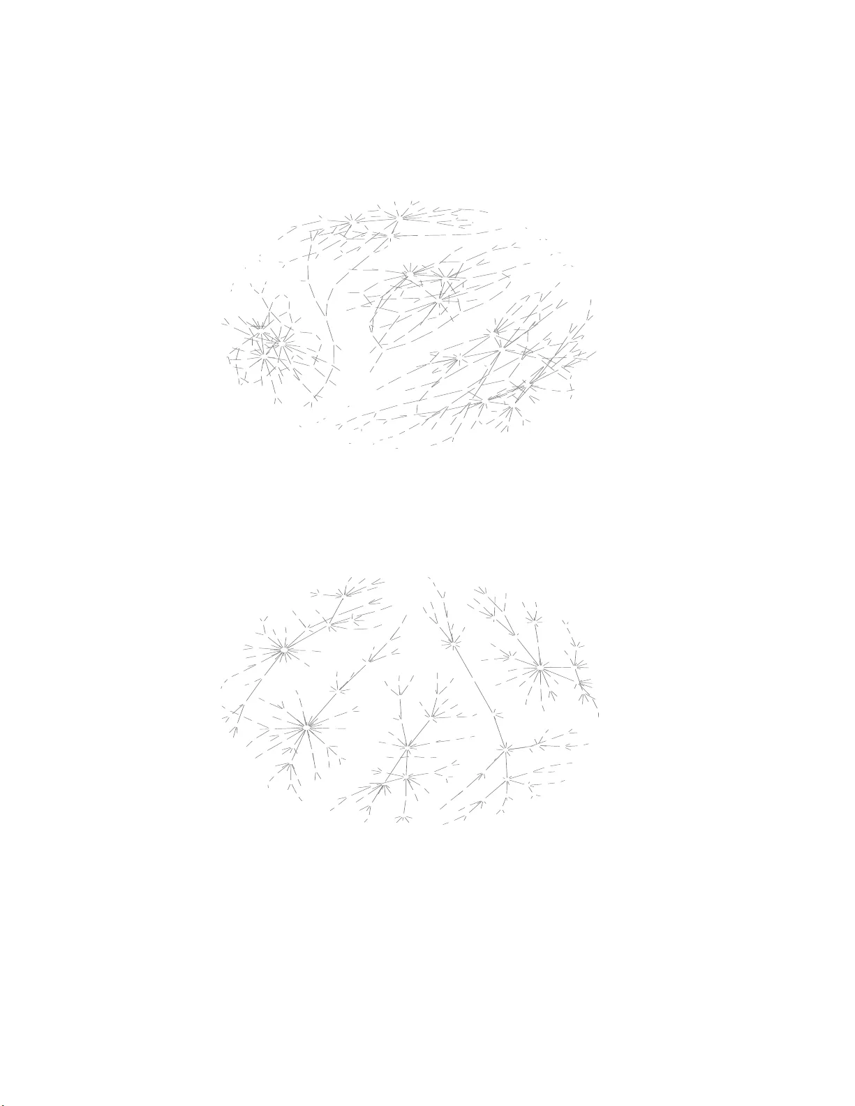
P artial Correlation Estimation b y Join t Sparse Regression Mo dels Jie P eng ∗ † , P ei W ang ∗‡ , Nengfeng Zhou § , Ji Zh u § † Department of Statist i cs, Univ ersity of C alifornia , Da vi s , CA 9561 6. ‡ Divisio n of Public Health Science, F red Hutchinson Cancer Researc h Center, Seattl e, W A 9810 9 . § Department of Statist i cs, U niv ersity of Mic h i gan, Ann Arb or, MI 4810 9 . ∗ Equal contributors † Corresp ondence author: jie@w ald.ucdavis.edu 1 Abstract In this pap er, w e prop ose a computationally eﬃcien t app roa ch — spa ce (Sparse P Artial Corr e lation Estimation)— for selecting n o n - zero partial correlat ions under th e high-dimens i on-low-sample-siz e setting. This metho d assumes the o v erall sparsit y o f the partial correlation m a trix and emplo ys sparse regression tec hniques for mo del ﬁtting. W e illustrate the p erformance of space b y exten- siv e simulatio n studies. It is sh o wn that spa ce perf o r ms w ell in b oth non-zero partial correlation selection and the identiﬁcat ion of h ub v ariables, and also out- p erforms tw o existing metho ds. W e then apply s pace to a microarra y breast cancer d a ta set and id e ntify a set of h u b genes whic h may p ro vide imp ortant insigh ts on genetic regulatory net works. Finally , we pro ve that, und e r a set of suitable assumptions, the prop osed pr o cedure is asymptotically consisten t in terms of mo del selection and parameter estimation. k ey w ords: concen tration netw ork, high-dimension-lo w-samp l e-size, lasso, sho oting, genetic regulatory net work 2 1 INTR ODUCTION There has been a large amoun t of literature on c ovarianc e sele ction : the iden tiﬁca- tion and estimation of non- z ero entrie s in the in verse co v ariance matrix (a.k.a. c onc en- tr ation matrix or pr e cision matrix ) starting from the seminal pap er by Dempster (1972). Co v ariance selection is v ery useful in elucidating associations among a set of ran- dom v ariables, as it is we ll known that non-zero en tries of the concen tratio n ma- trix corresp ond to non-zero partial correlations. Moreo v er, under G auss ianity , non- zero en tries of the concen tration matr ix imply conditional dependency b et w een cor- resp onding v ariable pairs conditional on the r est of the v a riables (Edward 2 0 00 ). T r aditional metho ds do es not w ork unless the sample size ( n ) is larger than the n um b er o f v ariables ( p ) (Whittak er 1990; Ed ward 2000). Recen tly , a n umber o f metho ds hav e b een intro d uced to p erform co v ariance selection for data sets with p > n , for example, see Meins ha u sen and Buhlmann (2 006), Y uan and Lin (20 0 7) , Li and G ui (2006), Sc hafer and Strimmer (2007 ) . In this pap er, w e prop ose a no ve l approac h using sparse regression tec hniques for co v ariance sele ction. Our work is partly motiv ated by the construction of genetic r e g u la tory networks ( GRN) based on high dimensional gene expression data . D enote the express io n lev els of p genes as y 1 , · · · , y p . A c onc entr ation network is deﬁned as an undirected gra ph, in whic h the p ve r tic es represen t the p genes and an edge connects gene i and gene j if and only if the partial correlatio n ρ ij b et w een y i and y j is non- zero. Note that, under the assumption tha t y 1 , · · · , y p are jo intly normal, t h e partial correlation ρ ij equals to Corr( y i , y j | y − ( i,j ) ), where y − ( i,j ) = { y k : 1 ≤ k 6 = i, j ≤ p } . Therefore, ρ ij b eing nonzero is equiv alen t to y i and y j b eing conditionally dep ende nt giv en all other v ariables y − ( i,j ) . The prop osed metho d is sp eciﬁcally designed for the high-dimension-lo w-sample-size scenario. It relies on the assumption that the partial correlation matrix is sparse (under normality a s sumption, this means t h a t 3 most v ariable pairs a r e conditionally indep e ndent), whic h is reasonable for many real life pro blems. F or instance, it has b een sho wn that mo st genetic net works are in trinsically sparse (Ga rdne r et al. 2003; Jeong et al. 2001; T egner et al. 2003). The prop osed method is also particularly p o we rf u l in the iden tiﬁcation o f hubs : v ertices (v ariables) tha t are connected to (ha ve nonzero partial correlatio n s with) man y other v ertices (v a riables ). The existenc e of h ubs is a w ell kno wn phenomenon fo r many large net w orks, suc h as the interne t , citation netw orks, and protein in t era ctio n netw orks (Newman 2003). In particular, it is widely b elie ved that genetic pa th w a ys consist of man y genes with few in teractions and a few hub genes with man y interactions (Barabasi and Oltv ai 2 004 ) . Another con tribution of this pa per is to prop ose a nov el a lg orithm active-shooting for solving p e nalized optimization pro b lems suc h as lasso ( Tibshirani 1996). This algorithm is computatio nally more eﬃcien t than the or ig inal shooting algor ithm , whic h w as ﬁrst prop osed by F u (1998 ) and then extended b y man y others including Genkin et al. (2007 ) and F riedman et al. (2007a). It enables us to implemen t the prop osed procedure eﬃcien tly , suc h that w e can conduct extensiv e sim ulation stud- ies in v olving ∼ 1000 v ariables and h undreds of samples. T o our kno wledge, t h is is the ﬁrst set o f in tensiv e sim ulation studies for co v ariance selection with suc h high dimensions. A few metho ds ha ve also b e en prop osed recen tly to perform co v ariance selection in the con text of p ≫ n . Similar to the metho d prop osed in this pap er, they all assume sparsit y of the partial correlation matrix. Meinshausen and Buhlmann (2 006) in tro duced a v ariable-b y-v ariable appro ac h for neighborho o d selection via the lasso regression. They pro ved that neighborho o ds can b e consisten tly selected under a set of suitable assumptions. How ev er, as regression mo dels are ﬁtted for eac h v ariable separately , this metho d has t w o ma jor limita t io ns . F irs t , it do es not take in to accoun t 4 the in trinsic symmetry of the problem (i.e., ρ ij = ρ j i ). This could result in loss o f eﬃciency , a s w ell as con tr a dic to r y neigh b orho o ds. Secondly , if the same p enalt y parameter is used fo r all p lasso regressions as suggested b y their pap er, more or less equal eﬀort is placed on building each neigh b orho o d. This apparently is not the most eﬃcien t w ay to address the problem, unless the degree distribution of the netw ork is nearly uniform. How ev er, most real life netw orks hav e sk ew ed degree distributions, suc h as the p ower-law networks . As observ ed by Sc hafer and Strimmer (2007), the neigh b orho o d selection approa c h limits the num ber of edges connecting to each no de. Therefore, it is not v ery eﬀectiv e in hu b detection. On the con tra ry , the prop osed metho d is based on a join t sparse regression mo del, whic h sim ultaneously p e r forms neigh b orho o d selection f o r all v ariables. It also preserv es the symmetry of the problem and th us utilizes data more eﬃcien tly . W e sho w by intens ive sim ulation studie s that our metho d p erforms b etter in b oth mo del selection and hub iden tiﬁcation. Moreov er, as a joint mo del is used, it is easier to incorp orate prior kno wledge suc h as net w ork top ology into the mo del. This is discussed in Section 2.1. Besides the regression approach men tioned ab o ve, another class of metho ds em- plo y t he maximum lik eliho od framew ork. Y uan and Lin ( 2 007) prop osed a p enal- ized maximum lik eliho o d approac h whic h p erforms mo del selection and estimation sim ultaneously and ensures the p ositiv e deﬁniteness of the estimated concen tration matrix. How ev er, their algorit hm can not handle high dimensional data. The largest dimension considered by them is p = 10 in sim ulatio n and p = 5 in real data. F riedman et al. (2 007b) prop osed an eﬃcie nt algorithm glasso to implemen t this metho d, such that it can b e applied to problems with high dimensions. W e sho w b y simulation studies that, the prop osed metho d p erforms b etter than glasso in b oth mo del selection and hu b identiﬁc a tion. Rothman et al (2008) prop osed an- other algorithm to implemen t t h e metho d of Y uan a nd L in (2007). The compu- 5 tational cost is on the same order of glasso , but in g eneral not as eﬃcien t a s glasso . Li and Gui (2006 ) in tro duced a threshold gradien t descen t (TGD) regu- larization pro cedure. Sc hafer a nd Strimme r (2007) prop osed a shrink age cov ariance estimation pro cedure to o v ercome the ill-conditioned problem of sample cov ariance matrix when p > n . There are also a large class of metho d s cov ering the situation where v ariables ha v e a natural ordering, e.g., long itud ina l data, time series, spatial data, or sp ectroscop y . See W u and Pourahmadi (200 3 ) , Bick el and Levina (20 0 8) , Huang et al. (200 6 ) and Levina et a l (2 006), whic h are all based on the mo diﬁe d Cholesky decomposition of the concentration matrix. In this pa per, w e, how ev er, fo cus on the general case where an ordering of the v ariables is not a v a ilable . The res t of the pap er is organized as follows. In Section 2, w e de scrib e the jo in t sparse regr ession mo del, its implemen tation a n d the active-shootin g a lg orithm. In Section 3 , the p erformance of the prop osed metho d is illustrated through sim ulatio n studies and compared with that of the neigh b orho od selec t io n approach and the lik eliho o d based approac h glasso . In Section 4, the prop osed metho d is applied to a microarray expression data set of n = 244 breast cancer tumor samples and p = 1217 genes . In Section 5, w e study the asymptotic prop erties of this pro cedure. A summary of the main r esults are giv en in Section 6. T ec hnique details are pro vided in the Supplemen tal Material. 2 METHOD 2.1 Mo del In this section, w e describe a no vel metho d for detecting pairs of v ariables ha ving nonzero partial correlations among a large num ber of r a nd o m v ariables based on i.i.d. samples. Supp ose that, ( y 1 , · · · , y p ) T has a join t distribution with mean 0 and co v ariance Σ , where Σ is a p b y p p ositiv e deﬁnite matrix. Denote the partial 6 correlation b et w een y i and y j b y ρ ij (1 ≤ i < j ≤ p ). It is deﬁned as Corr( ǫ i , ǫ j ), where ǫ i and ǫ j are the predic tio n errors of t he best linear predictors of y i and y j based on y − ( i,j ) = { y k : 1 ≤ k 6 = i, j ≤ p } , respectiv ely . Denote the c onc entr ation matrix Σ − 1 b y ( σ ij ) p × p . It is kno wn that, ρ ij = − σ ij √ σ ii σ j j . Let y − i := { y k : 1 ≤ k 6 = i ≤ p } . The follo wing w ell-known result (Lem ma 1) relates the estimation of par tial correlations to a regress ion problem . Lemma 1 : F or 1 ≤ i ≤ p , y i is expr esse d as y i = P j 6 = i β ij y j + ǫ i , such that ǫ i is unc orr elate d with y − i if an d only if β ij = − σ ij σ ii = ρ ij q σ j j σ ii . Mor e over, for such deﬁne d β ij , V ar( ǫ i ) = 1 σ ii , Cov( ǫ i , ǫ j ) = σ ij σ ii σ j j . Note that, under the normalit y assumption, ρ ij = Corr( y i , y j | y − ( i,j ) ) and in Lemma 1, w e can replace “uncorrelated” with “indep en dent”. Since ρ ij = sign ( β ij ) p β ij β j i , the searc h for non-zero partial corr elat io ns can b e view ed as a mo del selection problem under the regression setting. I n this pap er, w e are mainly interes ted in the case where the dimension p is larg e r than the sample size n . This is a typical scenario for many real life problems. F o r example, high t hro ughput genomic exp erimen ts usually result in dat a sets of thousands of genes for tens or at most hund r eds of samples. How ev er, man y high- dimensional problems are intrinsically sparse. In the case of genetic regulatory netw orks, it is widely believe d that most gene pairs are not directly in teracting with each other. Sparsit y suggests that ev en if the n umber of v ariables is m uch larg e r than t he sample size, the eﬀectiv e dimensionalit y of the problem migh t still b e within a tractable range. Therefore, w e prop ose to emplo y sparse regr ession tec hniques by imp osing the ℓ 1 p enalt y on a suitable loss function to tac kle the high- dim ension-low-sample-size problem. Supp ose Y k = ( y k 1 , · · · , y k p ) T are i.i.d. observ a t io ns f rom (0 , Σ ), for k = 1 , · · · , n . Denote the sample of the i th v ariable a s Y i = ( y 1 i , · · · , y n i ) T . Based on Lemma 1, w e 7 prop ose the following joint loss function L n ( θ , σ , Y ) = 1 2  p X i =1 w i || Y i − X j 6 = i β ij Y j || 2  = 1 2  p X i =1 w i || Y i − X j 6 = i ρ ij r σ j j σ ii Y j || 2  , (1) where θ = ( ρ 12 , · · · , ρ ( p − 1) p ) T , σ = { σ ii } p i =1 ; Y = { Y k } n k =1 ; and w = { w i } p i =1 are nonnegativ e w eights. F or example, w e can c ho ose w i = 1 / V ar( ǫ i ) = σ ii to weigh individual regressions in the joint loss function according to their residual v ariances, as is done in regression with heteroscedastic noise. W e prop ose to estimate the partial correlations θ b y minimizing a p enalized loss f u nction L n ( θ , σ , Y ) = L n ( θ , σ , Y ) + J ( θ ) , (2) where the p enalt y term J ( θ ) con tro ls the ov erall sparsit y of the ﬁnal estimation of θ . In this pa per, w e fo cus on the ℓ 1 p enalt y (Tibshirani 1996): J ( θ ) = λ || θ || 1 = λ X 1 ≤ i 0) . 2. F or j = 1 , ..., p , up date β ( old ) − → β ( new ) : β ( new ) i = β ( old ) i , i 6 = j ; β ( new ) j = arg min β j 1 2    Y − P i 6 = j β ( old ) i X i − β j X j    2 + γ | β j | = sign  ( ǫ ( old ) ) T X j X T j X j + β ( old ) j      ( ǫ ( old ) ) T X j X T j X j + β ( old ) j    − γ X T j X j  + , (5) where ǫ ( old ) = Y − X β ( old ) . 3. R e p eat step 2 un til c o n v ergence. A t eac h up dating step of the shooting algo rithm, w e deﬁne the set of curren tly non-zero co eﬃc ients as t he active set . Since under sparse mo dels, the activ e set should remain small, w e prop ose to ﬁrst up date the co eﬃ cients within the activ e set un til con v ergence is a chiev ed b efore mo ving on to up date o t her coeﬃcien ts. The active-shoo ting algo rithm pro ceeds as follow s: 1. Initia l ste p: same as the initial step of shooting . 13 2. D eﬁ ne the current a ctive set Λ = { k : curren t β k 6 = 0 } . (2 . 1) F or eac h k ∈ Λ , up date β k with all other co eﬃcien ts ﬁxed at the curren t v alue as in equation (5); (2 . 2) Rep eat (2.1) un til conv ergence is achiev ed on the activ e set. 3. F or j = 1 to p , update β j with all other co eﬃcien ts ﬁxed at the curren t v alue as in equation (5). If no β j c hanges during this pro cess, return the curren t β as the ﬁnal estimate. O t herwise, go bac k to ste p 2. T a ble 1: The num bers o f iterations required b y the shooting algorithm and the active-shoo ting alg o rithm to ac hiev e conv ergence ( n = 100, λ = 2). “co ef. #” is the n um b er of non-zero co eﬃcien ts p co ef. # shooting active-shooti ng 200 14 29600 4216 500 25 154000 10570 1000 28 291000 17029 The idea o f acti ve-shooting is to fo cus on the set of v ariables that is more lik ely to b e in the mo del, and th us it impro ve s the computational eﬃciency by ac hieving a faster conv ergence. W e illustrate the impro ve ment of the active-shooting ov er the shooting algorithm b y a small sim ulation study of the lasso regression (generated in the same wa y as in Section 5.1 o f F riedman et al. (2007a)). The tw o algorithms result in exact same solutions. How ev er, as can b e seen from T able 1, active-shooting tak es m uch fewe r iterations to con ve rg e (where one itera t io n is counted whenev er a n attempt to up date a β j is made). In particular, it take s less tha n 30 seconds (on a ve ra ge) to ﬁt the space mo del b y active-shooting (implemen ted in c co de) for cases with 1000 v ariables, 2 00 samples a nd when the resulting mo del has around 1000 non-zero pa r tial correlations on a serv er with tw o Dual/Core, CPU 3 GHz and 4 GB RAM. This great computational adv an tage enables us t o conduct large scale sim ulation s t udies to examine the p erformance of t h e pro posed metho d (Section 3). 14 Remark 1 : In the initial step, in s te ad of using the univariate soft-shrinka ge esti- mate, we c an use a pr evious estimate as the initial estim a t e if such a thing is available. F or e x a mple, when iter ating b etwe en { ρ ij } an d { σ ii } , we c an use the pr evious esti- mate of { ρ ij } in the curr ent iter ation as the initial val ue. This c an further impr ove the c omputational eﬃciency of the pr op ose d metho d, as a b etter initial value implies a faster c onver genc e. Mor e over, in pr actic e, o f ten estimates ar e de s ir e d for a series of tuning p ar ameters λ , w h et h e r it is for data explo r ation o r for the sele ction of λ . When this is the c ase, a de cr e asing-lamb da appr o ach c an b e use d to facilitate c omputation. That is, we start with the lar gest λ ( which r esults in the smal lest mo del), then use the r esulting estima te as the initial value when ﬁtting the mo del under the s e c ond lar gest λ and c ontinue i n this m a nner until al l estimates ar e o b t ain e d. 2.4 T uning The c hoice of the tuning parameter λ is of great imp ortance. Since the space metho d uses a lasso criterion, metho ds that hav e b een dev elop ed for selecting the tuning pa- rameter fo r lasso can a ls o b e applied to space , suc h as the G C V in Tibshirani (1996), the CV in F an a n d Li (2001 ) , the AIC in Buhlmann (2006) and the BIC in Zou et al. (2007). Sev eral metho ds ha ve also b een prop osed for selecting the tuning par a m eter in the set- ting of co v ariance estimation, f o r example, the MSE ba s ed criterion in Sc hafer and Strimmer (2007), the lik eliho o d based metho d in Huang et al. (2006) and the cross-v alidation and b oo t- strap metho ds in Li and G ui (200 6) . In this pap er, w e prop o s e to use a “BIC-t yp e” criterion for selecting the tuning para m eter mainly due to its simp licity and compu- tational easiness . F o r a giv en λ , denote the space es tima t o r b y b θ λ = { b ρ ij λ : 1 ≤ i < j ≤ p } and b σ λ = { b σ ii λ : 1 ≤ i ≤ p } . The corresp onding residual sum o f squares for the 15 i -th regression: y i = P j 6 = i β ij y j + ǫ i is RS S i ( λ ) = n X k =1   y k i − X j 6 = i b ρ ij λ s b σ j j λ b σ ii λ y k j   2 . W e then deﬁne a “BIC-type” criterion for the i -th regression as B I C i ( λ ) = n × log ( RS S i ( λ )) + log n × # { j : j 6 = i, b ρ ij λ 6 = 0 } . (6) Finally , we deﬁne B I C ( λ ) := P p i =1 B I C i ( λ ) and select λ b y minimizing B I C ( λ ). This metho d is referred to as space.joint hereafter. In Y uan a nd Lin (2 007), a BIC criterion is prop osed for the p enalized maxim um lik eliho o d approach. Namely B I C ( λ ) := n × h − log | b Σ − 1 λ | + trace( b Σ − 1 λ S ) i +log n × # { ( i, j ) : 1 ≤ i ≤ j ≤ p, b σ ij λ 6 = 0 } , (7) where S is the sample co v ariance matrix, and b Σ − 1 λ = ( b σ ij λ ) is the estimator un- der λ . In this pap er, we refer to this metho d as glasso.lik e . F or the purp ose of comparison, w e also consider t he selection of the tuning pa rame t er for MB . Since MB essen tially p erforms p individual lasso regressions, the tuning parameter can b e selected for eac h of them separately . Sp eciﬁcally , we use criterion (6) (ev aluated at the corresp onding MB estimators) to select the tuning parameter λ i for the i - th regression. W e denote this metho d as MB.sep . Alternativ ely , as suggested b y Meinshausen and Buhlmann (2006), when all Y i are standardized to ha v e sample standard deviation one, the same λ ( α ) = √ n Φ − 1 (1 − α 2 p 2 ) is applied to all r egr es- sions. Here, Φ is the standard normal c.d.f.; α is used to con trol the false disco v ery rate and is usually taken as 0 . 0 5 or 0 . 1. W e denote this metho d as MB.alpha . These metho ds are examined b y the sim ulatio n studies in the next section. 16 3 SIMULA TION In this section, w e conduct a series of simu la tion exp erime nts to examine the p erformance of the prop osed metho d space and compare it with the neigh b orho o d selection approac h MB as we ll a s t he p enalized likelihoo d metho d glasso . F or all three metho ds, v ariables are ﬁrst standardized to ha ve sample mean zero and sample standard deviation one b efore model ﬁtting . F or space , w e consider three diﬀeren t t yp es of weigh ts: (1) uniform w eights: w i = 1; (2) residual v ariance based w eights: w i = b σ ii ; and (3) degree ba sed we ig h ts: w i is pro portional to the estimated degree of y i , i.e., # { j : b ρ ij 6 = 0 , j 6 = i } . The corresponding metho ds are referred as space , space.sw and space.dew , resp ectiv ely . F or all three space metho ds, the initial v alue of σ ii is set to b e one. Iterations are used for these space metho ds as discus sed in Section 2.1. F or space.dew and space.sw , the initia l we ig hts are tak en to b e one (i.e., equal w eigh ts). In eac h subse quen t iteration, new w eigh ts are calculated based on the estimated residual v ariances (for space.sw ) or t h e estimated degrees (for space.dew ) of the previous iteration. F o r all three space methods, three iterations (that is up dating b et w een { σ ii } and { ρ ij } ) a r e used since the pro cedure con v erges v ery fast and more iterations result in essen tially the same estimator. F or glasso , the diagonal of the concen tration matrix is not p enalized. W e sim ulate net w or k s consisting of disjointed mo dules . This is done b ecause man y real life large net works exhibit a mo dular structure compris ed of man y disjointed or lo osely conne cted comp onen ts o f relativ ely small size. F o r example, exp erimen ts on mo del or ganism s like y east or bacteria suggest that the transcriptional regulatory net w orks ha v e mo dular structures (Lee et al. 2002). Eac h of our net w ork modules is set to hav e 100 no des and generated according to a give n degree distribution, where the de gr e e of a no de is deﬁned as the num b e r of edges connec ting to it. W e mainly consider tw o diﬀeren t types of degree distributions and denote their corresp onding 17 net w orks b y Hub network and Power-law network (details are give n later). Giv en an undirected netw ork with p no des, the initial “ concentration matrix” ( ˜ σ ij ) p × p is generated b y ˜ σ ij =            1 , i = j ; 0 , i 6 = j and no edge b et w een no des i and j ; ∼ U nif or m ([ − 1 , − 0 . 5] ∪ [0 . 5 , 1]) , i 6 = j and an edge connecting no des i and j . (8) W e then rescale the no n - ze ro elemen ts in the ab o v e matrix to assure p ositiv e deﬁnite- ness. Sp eciﬁcally , for eac h row, w e ﬁrst sum the a bs olute v alues of the oﬀ- diagonal en tries, and then divide each o ﬀ-diagonal entry by 1 . 5 fo ld of the sum. W e then av er- age this re-scaled matrix with its tr ans p ose to ensure symmetry . Finally the diago nal en tries are all set to b e one. This pro cess results in diagonal dominance. Denote t he ﬁnal matrix as A . The co v ariance matr ix Σ is then determined by Σ ( i, j ) = A − 1 ( i, j ) / p A − 1 ( i, i ) A − 1 ( j, j ) . Finally , i.i.d. samples { Y k } n k =1 are generated from Normal(0 , Σ ). Note that, Σ ( i, i ) = 1, and Σ − 1 ( i, i ) = σ ii ≥ 1. Sim ulation Study I Hub netw orks In the ﬁrst set of sim ulations, mo dule net w or ks are generated b y inserting a few h ub no des into a v ery sparse gra ph . Speciﬁcally , eac h mo dule consists of three h ubs with degrees around 15, and the other 97 no des with degrees at most four. This setting is designed to mimic the genetic regulatory net works , whic h usually con tains a few hub genes plus many other genes with only a few edges. A net w ork consisting of ﬁv e suc h mo dules is show n in Figure 1(a). In this net w ork, there are p = 500 no des and 568 edges. The sim ulated non-zero partial cor r elat io ns f all in 18 ( − 0 . 67 , − 0 . 1] ∪ [0 . 1 , 0 . 67), with t wo mo des a round - 0 .28 and 0.28. Based on this net w ork and the partia l correlation matrix, w e generate 50 indep enden t data sets eac h consisting of n = 250 i.i.d. samples. W e t h en ev aluate eac h metho d at a series of diﬀeren t v alues of the tuning param- eter λ . The num b e r of to tal detected edges ( N t ) decreases as λ increases. Figure 2 (a) sho ws the n umber of correctly detected edges ( N c ) vs. the num ber of total detected edges ( N t ) a ve ra ged across the 50 indep enden t dat a sets for eac h metho d. W e observ e that all three space methods ( space , space.sw and space.dew ) consisten tly de t ect more correct edges than the neighborho o d selection metho d MB (except for space.sw when N t < 470) a nd the lik eliho o d based method glasso . MB p erforms f av orably o ve r glasso when N t is relativ ely small (say less than 530), but p erforms w o r s e than glasso when N t is large. Ov erall, space.dew is the b est among all metho ds. Specif- ically , when N t = 568 (whic h is the num b e r of true edges), space.dew detects 501 correct edges on a verage with a standard deviation 4 . 5 edges. The corresp onding sen- sitivit y and sp eciﬁcit y are bot h 88%. Here, sensitivit y is deﬁned as the rat io of the n um b er of correctly detected edges to the total num b e r of true edges; and sp eciﬁcit y is deﬁned as the ra tio of the n umber of correctly detected edges to the n umber of total de tected edges. On the other hand, MB and gla sso detect 472 and 480 correct edges on av erage, resp ectiv ely , when t h e num b er of tota l detected edges N t is 5 68. In terms of h ub detection, for a giv en N t , a rank is assigned to eac h v ariable y i based on its estimated degree (the larger the estimated degree, the smaller the rank v alue). W e then calculate the a verage rank of the 15 true hu b no des for eac h metho d. The results are sho wn in Figure 2 (b). This a verage rank would ach ieve the minim um v alue 8 (indicated b y the grey horizon ta l line), if the 15 true hubs ha ve larger estimated degrees than all other non- h ub no des . As can b e seen from the ﬁgure, the a ve ra ge rank curv es (as a function of N t ) for the three space metho ds are very close to the o pt imal 19 minim um v alue 8 for a large range of N t . This suggests that these metho ds can success fully identify most o f the true h ubs. Indeed, for space.dew , when N t equals to the num ber of true edges (568), the top 1 5 no des with the highest estimated degrees con tain at least 14 out of the 15 true h ub no des in all replicates. On the other hand, b oth MB and glasso identify far f e wer h ub no des, as their corresp onding a verage rank curv es a r e muc h higher than the grey horizon ta l line. T a ble 2: P o wer (sensitiv ity) of space.dew , MB and glasso in identifying cor r ect edges when F D R is con trolled at 0 .05. Net w ork p n spa ce.dew MB glasso Hub-net w or k 500 250 0.844 0.784 0.655 200 0.707 0.656 0.559 Hub-net w or k 1000 300 0.85 6 0.790 0.690 500 0.963 0.894 0.826 P ow er-la w net w ork 500 250 0.704 0.667 0.580 T o in v estigate the impact o f dimensionality p and sample size n , w e p erform sim ulation studies for a larger dimension with p = 10 00 and v arious sample sizes with n = 200 , 300 and 500. The sim ulated net w ork includes ten disjoin ted mo dules of size 100 each and has 1163 edges in total. Non-zero partial correlations form a similar distribution as that of the p = 500 netw ork discussed abov e. The R OC curv es for space.dew , MB and glasso resulted f r om thes e sim ulations a re sho wn in Figure 3. When false disco v ery rate (= 1 -speciﬁcit y) is con trolled at 0 . 05, the p o w er (=sensitivit y) for detecting cor r ect edges is given in T able 2. F rom the ﬁgure and the table, w e observ e that the sample size has a big impact on the p erformance of all metho ds. F or p = 1000, when the sample size increases from 200 to 300, the p o wer of space.dew increases more than 20%; when the sample size is 50 0, space.dew ac hiev es an impressiv e p ow er of 96 % . On the other hand, the dimensionalit y seems to ha v e relativ ely less inﬂuen ce. When the total n umber of v ar ia ble s is doubled from 5 00 to 1000, with only 20 % more samples (that is p = 500 , n = 2 5 0 vs. p = 10 0 0 , n = 300), 20 all three metho ds ac hiev e similar p o wers . This is presumably b ecause the la r g e r net w ork ( p = 10 00) is sparser than the smaller netw ork ( p = 50 0 ) and also the complexit y of the mo dule s remains unchanged. Finally , it is ob vious from Figure 3 that, space.dew performs b est among the three metho ds. T a ble 3: Edge detection under the selected tuning parameter λ . F or ave r age r ank , the optimal v alue is 15 . 5 . F or MB.alpha , α = 0 . 05 is used. Sample size Metho d T otal edge detected Sen sit ivity S peciﬁcit y Av erage rank space.jo int 1357 0.821 0.703 28.6 n = 200 MB.sep 1240 0.75 1 0.703 57.5 MB.alpha 404 0.347 1.00 175.8 glasso.l ike 1542 0.821 0.619 35.4 space.jo int 1481 0.921 0.724 18.2 n = 300 MB.sep 1456 0.86 7 0.692 30.4 MB.alpha 562 0.483 1.00 128.9 glasso.l ike 1743 0.920 0.614 21 space.jo int 1525 0.980 0.747 16.0 n = 500 MB.sep 1555 0.94 0 0.706 16.9 MB.alpha 788 0.678 1.00 52.1 glasso.l ike 1942 0.978 0.586 16.5 W e then in v estigate the p erformance of these metho ds at the selected tuning pa- rameters (see Section 2.4 for details). F or the ab ov e Hub net w ork with p = 1000 no des and n = 200 , 300 , 500, the results are rep orted in T able 3. As can b e seen from the table, BIC based approaches tend to select large mo dels (compared to the true mo del whic h ha s 116 3 edges). space.joint and MB.sep p erform similarly in terms of sp eci- ﬁcit y , and glasso.like w orks considerably w orse tha n the other tw o in this regard. On the other hand, space.joint and glasso.like p erforms similarly in terms of sensitivit y , and are b etter than MB .sep on this asp ect. In contrast, MB.alpha selects v ery small mo dels and th us results in ve r y high sp eciﬁc ity , but v ery lo w sensitivit y . In terms of hub iden tiﬁcation, space.joint apparen tly p erforms b etter than other metho ds (indicated b y a smaller av erage rank ov er 30 true h ub no des). Moreo ver, the p erformances of all metho ds impro v e with sample size. 21 P ow er-la w net works Many real world net works ha v e a p ower-law (also a.k.a sc ale- fr e e) degree distribution with an estimated p o w er para meter α = 2 ∼ 3 ( Newman 2003). Th us, in the second set of sim ulations, the mo dule netw orks are generated according to a p o w er-law degree distribution with the p o w er- la w parameter α = 2 . 3, as this v alue is close to the estimated p o w er parameters for biological net w o rk s ( Newman 2003). Figure 1(b) illustrates a netw ork formed by ﬁv e suc h mo dules with eac h ha ving 100 no des. It can b e seen that there are three o b vious hub no des in this net w ork with degrees of a t least 20. The sim ulated non-zero partial correlatio ns fall in the range ( − 0 . 51 , − 0 . 08 ] ∪ [0 . 08 , 0 . 5 1 ), with t w o mo des around -0.22 and 0.22 . Similar to the sim ulation done fo r Hub netw orks, w e generate 50 indep end ent da ta sets eac h con- sisting of n = 250 i.i.d. samples. W e then compare the num ber of correctly detected edges by v arious metho ds. The result is sho wn in Figure 4. On a v era g e , when the n um b er of total detected edges equals to the n um b er of true edges whic h is 4 9 5, space.dew detects 406 correct edges, while MB detects only 378 and glasso de t ects only 381 edges. In terms of hub detection, all metho ds can corr ectly identify t h e three h ub no des for this net w ork. Summary These sim ulation results suggest that when the (concen tration) net w or k s are reasonably sparse, w e should b e able to c ha racte r ize their structures with only a couple-of-hundred s of samples when there are a couple of thousands of no des. In addition, space.dew outp erforms MB b y at least 6% on the p o w er o f edge dete ction under all sim ulat ion settings ab o v e when FDR is controlled at 0 . 05, a nd the improv e- men ts a re ev en larger when FDR is con trolled at a higher lev el say 0 . 1 (see Figure 3). Also, compared to glasso , the improv emen t of space. dew is at least 15% when FDR is controlled at 0 . 0 5, and the adv an tag es become smaller when FDR is controlled at a higher lev el (see Figure 3). Moreo v er, the space metho ds p erform m uch better in h ub iden tiﬁcatio n than b oth MB and glasso . 22 Sim ulation Study I I In the second sim ulation study , w e apply space , MB and glasso on net works with nearly uniform degree distributions generated b y follow ing the sim ulation pro cedures in Meins hausen and Buhlmann (2 006); as w ell as on the AR netw ork discuss ed in Y uan and Lin (2 007) and F riedman et a l. (2007b). F or these cases, space p e rf o rms comparably , if not better tha n , the other t wo metho ds. Ho we ver, for these net w orks without h ubs, the adv an tages o f space b ecome smaller compared to the results on the net w orks with hubs . The results are summarized b elo w. Uniform net works In this set of simulation, w e generate similar net w or ks a s the ones used in Meinshausen and Buhlmann (2006). These net w orks ha v e uniform degree distribution with degrees ranging from zero to fo ur. Figur e 5(a) illustrates a net work fo rme d by ﬁve suc h mo dules with each ha ving 100 no des. The re a re in total 4 4 7 edges. Figure 5(b) illustrates the p erformance of MB , space and glasso ov er 50 indep e ndent data sets eac h ha ving n = 250 i.i.d. samples . As can b e b een from this ﬁgure, all three metho ds p erform similarly . When the total n um b er o f detected edges equals to the tota l num ber o f true edges (447), space detects 372 true edges, MB detects 3 69 true edges and glasso 371 true edges. AR netw orks In this sim ulation, w e consider the so called AR netw ork used in Y uan and Lin (2 007) and F riedman et al. (2007b). Sp e ciﬁcally , we ha v e σ ii = 1 for i = 1 , · · · p and σ i − 1 ,i = σ i,i − 1 = 0 . 25 for i = 2 , · · · , p . Fig ur e 6(a) illustrates suc h a net w ork with p = 500 no d es and thus 499 edges. Figur e 6(b) illustrates the p erfor- mance of MB , space and glasso ov er 5 0 indep ende nt data sets eac h ha ving n = 250 i.i.d. samples . As can b e b een from this ﬁgure, all three metho ds ag a in p erform similarly . When the total num b er of detected edges equals to the to tal num b e r of true edges (49 9), space detects 416 t r ue edges, MB detects 41 7 true edges and glasso 411 true edges. As a slight mo diﬁcation of the AR netw ork, w e a ls o consider a big 23 circle netw ork with: σ ii = 1 for i = 1 , · · · p ; σ i − 1 ,i = σ i,i − 1 = 0 . 3 fo r i = 2 , · · · , p and σ 1 ,p = σ p, 1 = 0 . 3. Figure 7(a) illustrates suc h a net w o rk with p = 50 0 no des and th us 500 edges. Figure 7 (b) compares the p erformance of the three metho ds . When the total num b e r of detected edges equals to the total n umber of tr ue edges (500 ), space , MB and glasso detect 4 7 8, 478 and 475 true edges, resp ectiv ely . W e also compare the mean squared error (MSE) of estimation of { σ ii } . F or the uniform net w ork, the median (across all samples and λ ) of the square-ro ot MSE is 0 . 108 , 0 . 113 , 0 . 1 78 for MB , space and glasso . These n um b ers are 0 . 085 , 0 . 089 , 0 . 142 for the AR netw ork and 0 . 128 , 0 . 138 , 0 . 233 for t he circle net w ork. It seems that MB and space w ork considerably b etter than glasso on this asp ect. Commen ts W e conjecture that, under the sparse and high dimensional setting, t he sup erior p erformance in mo del selection of the regression based metho d space o ver the p e- nalized lik eliho o d metho d glasso is pa r t ly due to its simpler quadratic loss function. Moreo v er, since space ignores the correlation structure of the regression residuals, it amoun ts to a greater degree of regularization, whic h ma y render additional b eneﬁts under t he sparse and high dimensional setting. In terms of para m eter estimation, w e compare the entrop y loss of the three meth- o ds. W e ﬁnd that, they p erform similarly when the estimated mo dels are of small or mo derate size. When the estimated mo dels are larg e , glasso generally p e rf o rms b etter in this regard than the other tw o metho ds. Since the in terest of this pap er lies in mo del selection, detailed r esults o f pa rame t er e stimatio n are not rep orted here. As discussed earlier, one limitatio n of space is its lack o f assurance o f p ositiv e deﬁniteness . Ho we ver, for sim ulations repo rted ab o v e, the corresp onding estimators w e hav e examined (ov er 3000 in tota l) a re a ll p ositiv e deﬁnite. T o further in ves tig a te 24 this issue, we design a few additional sim ulations. W e ﬁrst consider a case with a similar netw ork structure as the Hub net work, how ev er having a nearly singular concen tration ma t rix (the condition num b er is 16 , 2 4 0; a s a comparison, the condition n um b er fo r the or ig inal Hub net work is 62). F or this case, the estimate of space remains p ositiv e deﬁnite un t il the num ber of to t al detected edges increases to 50 , 000; while the estimate o f MB remains p ositiv e de ﬁnite un til the n um b er of total detected edges is more than 23 , 000. Note that, the total n umber of true e dg es of this model is only 568, and the mo del selecte d b y space.joint has 791 edges. In the second sim ulation, w e consider a denser netw ork ( p = 500 and the num b e r of true edges is 6 , 188 ) with a nearly singular concen tration matrix (condition n umber is 3 , 669). Again, we o bserv e that, the space estimate only b ecome s non- positiv e-deﬁnite whe n the estimated mo de ls are huge (the n um b er of detec ted edges is more than 45 , 000). This suggests that, for the regime we are in terested in in this pap e r (the sparse and high dimensional setting), non-p ositiv e-deﬁniteness do es not seem to b e a big issue for the prop osed metho d, as it only o ccurs when t h e resulting mo del is h uge and th us v ery far aw a y from the true mo del. As long as the estimated mo dels are reasonably sparse, the correspo nd ing estimators b y space remain p ositiv e deﬁnite. W e b eliev e that this is partly due to the he avy shrink age imposed on the oﬀ- dia gonal en t r ies in order to ensure sparsit y . Finally , w e inv estigate the p erformance of these metho ds when the observ atio n s come fro m a non- normal distribution. P articularly , w e consider the m ultiv ariate t d f - distribution with d f = 3 , 6 , 10. The p erformances of all three metho ds deteriorate compared to the no rm a l case, how ev er the ov erall picture in terms o f r elat ive p erfor- mance a mo ng thes e methods remains essen tially unc hanged (T able 4). 25 T a ble 4: Sensitivit y of diﬀeren t metho ds under diﬀeren t t d f -distributions when FDR is controlled at 0.05 Sensitivit y df Metho d Hub Po w er-la w space 0.369 0.286 3 MB 0.388 0.276 glasso 0.334 0.188 space 0.551 0.392 6 MB 0.535 0.390 glasso 0.471 0.293 space 0.682 0.512 10 MB 0.639 0.518 glasso 0.598 0.345 4 APPLICA TION More than 500,000 w omen die a n nually of breast cancer w or ld wide. Great eﬀorts are b eing made to improv e the prev en t io n, diagnosis and treatmen t for breast cancer. Sp ec iﬁcally , in the past couple o f ye a r s, molecular diagnostics of breast cancer ha v e b een rev olutionized by high throughput genomics tec hnologies. A large n umber of gene expression signatures hav e b een iden tiﬁed (or ev en v alidated) to ha ve p oten tial clinical usage. How ev er, since breast cancer is a complex disease, the tumor process cannot b e understo o d b y only analyzing individual genes. There is a pressing need to study the in teractions b et w een genes, whic h ma y w ell lead to b etter understanding of t he disease patho logies . In a recen t breast cancer study , microarray expression experiments w ere conducted for 295 prima r y inv asiv e breast carcinoma samples (Chang et al. 2 005 ; v an de Vijv er et al. 2002). Ra w array data and patient clinical outcomes for 24 4 of these samples are av ailable on- line and are used in this pap er. Data can b e do wnloaded at http://microarra y-pubs.stanford.edu/wou n d N K I / e x p l o r e . h t m l . T o globally c haracterize the asso ciation a m o ng thousands of mRNA expression lev- els in this gro up of patients , w e a pply the space me tho d on this data set as follow s. First, for each express io n array , we p erform the global normalizatio n b y cen tering the 26 mean to zero and scaling the median absolute deviation to one. Then w e fo cus on a subset of p = 1217 genes/clones whose expression lev els are signiﬁcantly asso ciated with tumor progression ( p -v alues from univ ariate C ox mo dels < 0.0 008, corresp ond- ing FDR = 0 . 01). W e estimate t he partial correlation matrix of these 12 17 genes with space.dew for a series of λ v alues. The degree distribution of the inferred netw ork is hea vily sk ewe d to the righ t. Sp eciﬁ cally , when 629 edges a re detected, 5 98 out of the 1217 genes do not connect to an y other genes, while ﬁv e genes ha ve degrees of at least 10. The pow er-la w parameter of this degree distribution is α = 2 . 56 , whic h is con- sisten t with the ﬁndings in the literature for G R N s (Newman 2003). The topolo gy of the inferred net w ork is sho wn in Figure 8(a), whic h supp orts the statemen t that genetic path w ays consist of man y genes with few in teractions and a few h ub genes with man y interactions. W e then searc h for p oten tial h ub genes by ranking no des according to their de- grees. There are 11 candidate hub g e nes whose degrees consisten tly rank the highest under v arious λ [see Figure 8 (b)]. Among these 11 genes , ﬁve are imp ortant know n regulators in breast cancer. F or example, HNF3A (also kno wn as FO XA1 ) is a transcription factor expressed predominan tly in a subt yp e of breast cancer, whic h regulates the express io n of the cell cycle inhibitor p 27 k ip 1 and the cell adhesion molecule E-cadherin. This gene is essen tial for the ex pression of a pp r oximately 50% of estrogene-regulated genes and has the p oten tial to serv e as a therap eutic target (Nakshatri and Badv e 2007). Except for HNF3A , all the other 10 hub genes fall in the same big netw ork comp onen t related to cell cycle/proliferation. This is not surpris- ing as it is w ell-ag re ed that cell cycle/proliferation signature is progno s tic for breast cancer. Sp e ciﬁcally , KNSL6, STK12, RAD54L and BUB1 ha v e b ee n previously re- p orted to play a role in breast cancer: KNSL6 (also kno wn as KIF2C ) is imp ortan t for anaphase chromosome segregatio n and centromere separation, which is ov erexpres sed 27 in breast cancer cells but expressed undetectably in other h uman tissues except testis (Shimo et al. 2 008 ) ; STK1 2 (also kno wn as A URKB ) regulates c hromosomal segre- gation during mitosis as we ll as meiosis, whose LOH con tributes to an increased breast cancer risk and ma y inﬂuence the therapy outcome (Tc hatchou et al. 2007); RAD54L is a recom binatio na l repair protein asso ciated with tumor suppressors BRC A1 and BR CA2, whose mutation leads to defect in repair pro cesses inv olving homologous re- com bination and t r ig gers the tumor dev elopmen t (Matsuda et al. 1999); in the end, BUB1 is a spindle c hec kp oin t gene and b elongs to the BML-1 oncogene-driv en path- w ay , whose a ctiv ation contributes to the surviv al life cycle of cancer stem cells and promotes tumor progression. The roles of the other six h ub genes in breast cancer are w orth of further in v estigatio n. The functions of all h ub genes are brieﬂy summarized in T able 5 . T a ble 5: Annota tion of h ub genes Index Gene Sym b ol Summary F unction (GO) 1 CENP A Enco des a cen tromere protein (nuc leosome assem bly) 2 NA. Annotation not available 3 KNSL6 Anaphase c hromosome se gr e ga tion (cell proliferation) 4 STK12 Regulation of chromosomal segregatio n (ce ll c ycle) 5 NA. Annotation not available 6 URLC9 A nn ot ation not available (up-r egula te d in lung cancer) 7 HNF3A T ranscriptional factor activit y (epithelial cell diﬀerentiation) 8 TPX2 Spindle formation (cell proliferatio n) 9 RAD54L Homologous recom bination related D NA repair (meiosis) 10 ID-GAP Stim ulate GTP h ydrolysis (cell cycle) 11 BUB1 Spindle c hec kp oin t (cell cycle) 5 ASYMPTOTICS In t his section, w e sho w that under appropriate c o nd it io ns , the space pro cedure ac hiev es b oth mo del selection consistency and estimation consistency . Use θ and σ to 28 denote t h e tr ue parameters of θ and σ . As discussed in Section 2.1, when σ is give n, θ is estimated by solving the following ℓ 1 p enalization problem: b θ λ n ( σ ) = arg min θ L n ( θ , σ , Y ) + λ n || θ || 1 , (9) where the loss func tion L n ( θ , σ , Y ) := 1 n P n k =1 L ( θ , σ , Y k ) , with, for k = 1 , · · · , n L ( θ , σ , Y k ) := 1 2 p X i =1 w i ( y k i − X j 6 = i p σ j j /σ iiρ ij y k j ) 2 . (10) Throughout this section, we assume Y 1 , · · · , Y n are i.i.d. samples from N p (0 , Σ ). The G a us sianity assumption here can b e r e laxed by assuming appropriat e tail b e- ha viors of the observ ations. The assumption of zero mean is simply for exp osition simplicit y . In practice, in the lo ss function (9), Y k can b e replaced b y Y k − Y where Y = 1 n P n k =1 Y k is the sample mean. All results stated in this section still hold under that case. W e ﬁrst state r e gula rit y conditions that are needed for the pro of. Deﬁne A = { ( i, j ) : ρ ij 6 = 0 } . C0: The w eights satisfy 0 < w 0 ≤ min i { w i } ≤ max i { w i } ≤ w ∞ < ∞ C1: There exist constan ts 0 < Λ min ( θ ) ≤ Λ max ( θ ) < ∞ , suc h that the true co v ariance Σ = Σ ( θ , σ ) satisﬁes: 0 < Λ min ( θ ) ≤ λ min ( Σ ) ≤ λ max ( Σ ) ≤ Λ max ( θ ) < ∞ , where λ min and λ max denote the smallest and largest eigen v alues of a ma t r ix , resp e ctive ly . C2: There exist a constan t δ < 1 such that for all ( i, j ) / ∈ A     L ′′ ij, A ( θ , σ ) h L ′′ A , A ( θ , σ ) i − 1 sign( θ A )     ≤ δ ( < 1) , 29 where for 1 ≤ i < j ≤ p, 1 ≤ t < s ≤ p , L ′′ ij,ts ( θ , σ ) := E ( θ ,σ )  ∂ 2 L ( θ , σ , Y ) ∂ ρ ij ∂ ρ ts    θ = θ,σ = σ  . Condition C0 sa ys that the w eights are b ounded a w a y from zero and inﬁnit y . Con- dition C1 assumes that the eigen v alues of the true cov ariance matrix Σ are b ounded a wa y from zero and inﬁnit y . Condition C2 corresp onds to the inc oher enc e c on dition in Meinshausen and Buhlmann (2 006), whic h pla ys a crucial role in pro ving mo del selection consistency of ℓ 1 p enalization problems. F urthermore, since σ is usually unkno wn, it needs to b e estimated. Use b σ = b σ n = { b σ ii } p i =1 to denote one estimator. The following condition says D : F or any η > 0, there exis ts a constan t C > 0, suc h that f o r suﬃcien tly large n , max 1 ≤ i ≤ p | b σ ii − σ ii | ≤ C ( q log n n ) holds with probabilit y at least 1 − O ( n − η ). Note that, the t heorems b elo w hold eve n when b σ is obtained based on the same data set fro m whic h θ is estimated as lo ng as condition D is satisﬁed. The follo wing prop osition says that, when p < n , w e can get a n estimator of σ satisfying condition D by simply us ing the residuals of the ordinary least square ﬁtting. Prop osition 1 Supp ose Y = [ Y 1 : · · · : Y n ] is a p × n data matrix with i.i.d. c olumns Y i ∼ N p (0 , Σ ) . F urt h e r supp ose that p = p n such that p/n ≤ 1 − δ for s o me δ > 0 ; and Σ has a b ounde d c ondition numb er (that is assuming c ondition C1). L et σ ii denote the ( i, i ) -th eleme n t o f Σ − 1 ; and let e i denote the r esidual fr om r e gr essing Y i on to Y ( − i ) := [ Y 1 : · · · : Y i − 1 : Y i +1 : · · · : Y n ] , that is e i = Y i − Y T ( − i ) ( Y ( − i ) Y T ( − i ) ) − 1 Y ( − i ) Y i . 30 Deﬁne b σ ii = 1 / b σ ii, − ( i ) , wher e b σ ii, − ( i ) = 1 n − p − 1 e T i e i , then c ondi t ion D holds for { b σ ii } p i =1 . The pro of of this prop osition is omitted due to space limitation. W e no w state not a tions used in the main results. Let q n = | A | denote the n um- b er of nonzero pa rtial correlations (of the underlying t rue mo del) and let { s n } b e a p ositiv e sequence of real n umbers such that for an y ( i, j ) ∈ A : | ρ ij | ≥ s n . Note that, s n can b e view ed as the signal size. W e follow the similar strategy as in Meinshausen and Buhlmann (2006) and Massam et al. (2 007) in deriving the asymp- totic result: (i) First prov e estimation consistency a nd sign consistency for the re- stricted p enalization problem with θ A c = 0 (Theorem 1). W e emplo y the metho d of the pro of of Theorem 1 in F an and P eng ( 2 004); (ii) Then w e pro ve that with probabilit y tending to one, no wrong edge is selecte d (Theorem 2); (iii) The ﬁnal consistency result then follows (Theorem 3). Theorem 1 (c onsistency of the r estricte d pr oblem) Supp ose that c onditions C0-C1 and D ar e satisﬁe d. Supp ose further that q n ∼ o ( q n log n ) , λ n q n log n → ∞ and √ q n λ n ∼ o (1) , as n → ∞ . Then ther e exis t s a c onstant C ( θ ) > 0 , such that for an y η > 0 , the fol lowing events hold with pr ob ability at le ast 1 − O ( n − η ) : • ther e exists a solution b θ A ,λ n = b θ A ,λ n ( b σ ) o f the r estricte d pr oblem: min θ : θ A c =0 L n ( θ , b σ , Y ) + λ n || θ || 1 , (11) wher e the loss function L n is deﬁne d via (10). • (e st im at i o n c onsistency) any solution b θ A ,λ n of the r estricte d pr oblem (11) satis- 31 ﬁes: || b θ A ,λ n − θ A || 2 ≤ C ( θ ) √ q n λ n . • (s ign c onsistency) if further a ssume that the signal se quenc e satisﬁes: s n √ q n λ n → ∞ , n → ∞ , then sign ( b θ A ,λ n ij ) = sign( θ ij ) , for al l 1 ≤ i < j ≤ p . Theorem 2 Supp ose that c onditions C 0-C2 and D ar e sa tisﬁ e d. S u pp ose further that p = O ( n κ ) for som e κ ≥ 0 ; q n ∼ o ( q n log n ) , q q n log n n = o ( λ n ) , λ n q n log n → ∞ and √ q n λ n ∼ o (1) , as n → ∞ . Then for any η > 0 , for n suﬃciently lar ge, the solution of (11) satisﬁes P ( θ , σ )  max ( i,j ) ∈A c | L ′ n,ij ( b θ A ,λ n , b σ , Y ) | < λ n  ≥ 1 − O ( n − η ) , wher e L ′ n,ij := ∂ L n ∂ ρ ij . Theorem 3 Assume the same c onditions o f T he or em 2. Then ther e e x ist s a c onstant C ( θ ) > 0 , such that fo r any η > 0 the fol low ing ev e nt s hold with p r ob ability at le ast 1 − O ( n − η ) : • ther e exists a solution b θ λ n = b θ λ n ( b σ ) of the ℓ 1 p enalization pr oblem min θ L n ( θ , b σ , Y ) + λ n || θ || 1 , (12) wher e the loss function L n is deﬁne d via (10). • (e st im at i o n c onsistency): any solution b θ λ n of (12) satisﬁes: || b θ λ n − θ || 2 ≤ C ( θ )( √ q n λ n ) . 32 • (Mo del sele ction c onsistency/sign c onsistenc y ): sign( b θ λ n ij ) = sign( θ ij ) , fo r al l 1 ≤ i < j ≤ p. Pro ofs of these theorems are giv en in the Supplemen tal Material. Finally , due to exponential small t a ils of the probabilistic b ounds, mo del sele ctio n consistency can b e easily e xtended when the net work consists of N disjointed compo nents with N = O ( n α ) fo r some α ≥ 0, as lo ng as the size and the num b er of true edges of eac h comp onen t satisfy the corresp onding conditio n s in Theorem 2. Remark 2 The c ondition λ n q n log n → ∞ is inde e d impli e d b y the c ondition q q n log n n = o ( λ n ) as long as q n do es not go t o zer o. Mor e over, under the “worst c ase” sc enario , that is when q n is alm o s t in the or der of q n log n , λ n ne e ds to b e ne arly in the or de r of n − 1 / 4 . On the other hand, for the“b est c ase” sc enario, that is when q n = O ( 1 ) (for example, when the dime nsion p is ﬁxe d), the or der of λ n c an b e ne arly as smal l as n − 1 / 2 (within a factor of log n ). Conse quently, the ℓ 2 -norm d ist a n c e of the estimator fr om the t rue p ar ameter is in the o r der of p log n/n , w it h pr ob ab i l i ty tending to one. 6 SUMMAR Y In this pap er, w e pro p ose a join t sparse regression mo del – space – for select- ing non-zero partial correlations under the high-dimension-low - s a mple-size setting. By con tro lling the o v erall sparsit y o f the partia l correlation matrix, space is able to automatically adjust for diﬀeren t neigh b orho o d sizes and th us to utilize data more eﬀectiv ely . The prop osed metho d also explicitly employs t he symmetry a m o n g the partial correlations, whic h also helps to improv e eﬃciency . Moreo v er, this joint mo del mak es it easy to incorp orate prior knowle dge ab out netw ork structure. W e dev elop a fast algor it hm active-shooti ng to implemen t t he prop osed pro cedure, whic h can b e 33 readily extended to solve some other p enalized optimizatio n problems. W e a lso pro- p ose a “BIC-type” criterion fo r the selection o f the tuning parameter. With extensiv e sim ulation studies, w e demonstrate tha t this metho d a c hiev es go o d p o w er in non-zero partial correlation selection a s w ell as h ub identiﬁcation, and a ls o p erforms fav orably compared to tw o existing metho ds. The impact of the sample size and dimensionality has b een examined o n simu la tion examples a s w ell. W e then apply this metho d on a microarra y data set of 1217 genes from 244 breast cancer tumor samples, and ﬁnd 11 candidate h ubs, of whic h ﬁve are kno wn breast cancer related regulators. In the end, w e show consistency (in terms of mo del selection and estimation) of the prop osed pro cedure under suitable r egula r ity and sparsity conditions. The R pac k age sp ac e – Sparse P Artial Correlatio n Estimation – is a v ailable on cran . A CKNO WLEDGEMENT A pap er based on this rep ort has b een accepted for publication on Journal of the American Statistical Asso ciation ( http://www.amstat.or g/pu blications/JASA/ ). W e are grat eful to tw o anon ymous review ers and an asso ciate editor for their v aluable commen ts. P eng is partially suppo rted b y grant DMS-080612 8 from t he Natio nal Science F oundation and grant 1R01GM082802-0 1A1 from the Natio nal Institute of General Medical Sciences . W ang is partially supp orted by gran t 1R01GM082802-0 1A1 from the National Institute of General Medical Sciences. Zhou and Zhu are partia lly sup- p orted b y grants D MS-0505432 and DMS-070553 2 fro m the National Scie nce F oun- dation. 34 References Barabasi, A. L., and Alb ert, R. (199 9 ), “Emergence o f Scaling in Random Net- w orks,” Sc i e nc e , 286, 509– 512. Barabasi, A. L., and Oltv ai, Z. N. ( 2004), “Netw ork Biolo gy: Understanding the Cells F unctional Organization,” Natur e R evi e w s Genetics , 5, 101–113. Bic k el, P .J., and Levina, E. (2008), “Regularized Estimation of Large Co v a riance Matrices,” Annals of Statistics , 36, 1 99–227. Buhlmann, P . (2 006), “Bo osting for High-dimensional Linear Mo dels,” Annals of Statistics , 34, 559–5 8 3. Chang, H. Y., Nuyten, D. S. A., Sneddon, J. B., Hastie, T., Tibshirani, R., Sorlie, T., Dai, H., He,Y., v an’t V eer, L., Bartelink, H., and et al. (2005), “Robustness, Scalabilit y , and In tegration of a W ound Resp o nse Gene Expression Signat ure in Predicting Surviv al of Human Breast Cancer Patien ts,” Pr o c e e dings of the National A c ademy of Scienc es , 8 ;102(10): 3738-43 . Dempster, A. ( 1972), “Co v ariance Selection,” Bio metrics , 28, 157–175 . Edw ard, D. (2000), Intr o d uction to Gr aphic al Mo del ling (2nd ed.), New Y or k: Springer. Efron, B., Hastie, T., Johnstone, I., and Tibshirani, R. (2004), “L east Angle R e- gression,” Annals of Stat i s tics , 32, 407–4 99. F an, J., a nd Li, R . (2 0 01), “V ariable Selection via Nonconca ve P enalized Likeli- ho o d and Its Oracle Prop erties,” Journal o f the Americ an Statistic al Asso cia- tion , 96, 1348–136 0 . F an, J., and P eng, H. (20 0 4), “ Nonconca v e P enalized L ikelihoo d with a Dive r ging Num b er of P ara mters,” A nna ls of statistics , 32(3), 928–96 1 . 35 F riedman, J., Hastie, T., Hoﬂing, H., and Tibshirani, R. (200 7a), “P athwis e Co or- dinate Optimization,” Annals of Applie d Statistics , 1(2), 302-33 2 . F riedman, J., Hastie, T., and Tibshirani, R. (20 07b), “Spar se In- v erse Co v ariance Estimation with the G raphical Lasso,” Biostatis- tics doi:10.1 093/biostatistics/kxm045. F riedman, J., Hastie, T., and Tibshirani, R. (20 0 8), “ Regularization P aths for Generalized Linear Mo dels via Co ordinate D escen t,” T e chnic al r ep ort: http://www-stat.stanfor d.e du/ ∼ jhf/ftp/glmnet.p df . F u, W. (199 8 ), “Pe nalized Regr essions: the Bridge vs the Lasso,” Journal o f Com - putational and Gr aphic al Statistics , 7(3), 397–416. Gardner, T. S., Bernardo, D. di, Lorenz, D., and Collins, J. J. (2003), “ Inferring Genetic Net w orks and Iden tifying Comp ound Mo de of Action via Expression Proﬁling,” Scienc e , 301, 102–105. Genkin, A., Lewis, D . D, and Madiga n, D. (200 7 ), “ L a rge-Scale Ba yes ia n Logistic Regression for T ext Categorization,” T e chnome trics , 49, 291– 304. Huang, J., Liu, N., P ourahmadi, M., and Liu, L . (2 006), “ Co v ariance Matrix Selec- tion and Estimation via P enalised Normal Lik eliho o d,” B iometrika , 93, 85–98. Jeong, H., Mason, S. P ., Barabasi, A. L., and Oltv ai, Z. N. (2001 ), “Lethality and Cen trality in Protein Ne tw orks,” Natur e , 411, 41–42. Lee, T. I., Rinaldi, N. J., Ro b ert, F., Odom, D. T., Bar-Joseph, Z., Gerb er, G. K., Hannett, N. M., Har bison, C. T., Thompson, C. M., Simon, I., Z eitlinger, J., and et al. (20 0 2), “T ranscriptional Regulatory Netw orks in Sacc haromyc es Cerevisiae,” Scienc e , 298, 799–804. Levina, E. and Rothman, A. J. and Zhu, J. (2 0 06), “Sparse Estimation of Large Co v ariance Matrices via a Nested Lasso P enalty ,” Biometrika , 90, 831–84 4. 36 Li, H., and Gui, J. (200 6 ), “Gradient Directed Regularization for Sparse Gaussian Concen tration Graphs, with Applications to Inference of Genetic Netw orks,” Biostatitics , 7(2 ) ,302 –317. Massam, H., P aul, D., and Ra jaratnam, B. (2 007), “Penalize d Empirical Risk Minimization Using a Conv ex Lo ss F unction a nd ℓ 1 P enalt y ,” Unpublishe d Manuscript . Matsuda, M., Miy agaw a, K., T ak ahashi, M., F ukuda, T., Ka taok a, T., Asahara, T., In ui, H., W ata t a ni, M., Y asutomi, M., Ka mada, N., Dohi, K., a nd Kamiy a, K. (1999), “Mutations in t he Rad5 4 Recom bination Gene in Primary Cancers,” Onc o gene , 18, 3427– 3430. Meinshausen, N., and Buhlmann, P . (20 06), “High Dimensional G raphs and V ari- able Selection with the Lasso,” Annals of Statistics , 34, 1436-1462. Nakshatri, H., and Badve , S. (2 0 07), “F OXA1 as a T herap eutic T arget for Breast Cancer,” Exp ert Opinion o n Ther a p eutic T ar gets , 11, 507–51 4. Newman, M. (2003) , “The Structure and F unction of Complex Net w o rks,” So ciety for Industrial and Applie d Mathematics , 45(2), 167– 256. Rothman, A. J. and Bick el, P . J. and Levina, E. and Z hu, J. (2008), “Sparse p erm u- tation in v ariant co v ariance estimation,” Ele ctr onic Journal of Statistics , 2 , 4 94– 515. Sc hafer, J., and Strimmer, K. (2007), “A Shrink a g e Approac h to Large-Scale C o - v ariance Matrix Estimation and Implications for F unctional Genomics,” Statis- tic al Applic ations in Genetics and Mole cular Biolo gy , 4 ( 1 ), Article 32 . Shimo, A., T anik a w a, C., Nishidate, T., Lin, M., Matsuda, K., Park, J., Uek i, T., Oh ta, T., Hirata, K., F ukuda, M., Na k am ura , Y., a nd Katagiri, T. (20 0 8), “In- v olv emen t of Kinesin F a mily Mem b er 2C/Mitotic Cen tromere-Asso ciated Ki- 37 nesin O verex pression in Mammary Carcinogenesis,” Canc er Scienc e , 99(1 ) , 62– 70. Tc hatc hou, S., Wirten b erger, M., Hemmink i, K., Sutter, C., Meindl, A., W ap- p ensc hmidt, B., Kiech le, M., Bugert, P ., Sc hmutzler, R., Bar t r a m, C., and Burwink el, B. (20 0 7), “Aurora Kinases A and B and F amilial Breast Cancer Risk,” Canc er L etters , 24 7(2), 266 –272. T egner, J., Y eung, M. K., Hasty , J., and Collins, J. J. (2003 ), “Reve rse Engineering Gene Net w o rks: In tegra ting Genetic Pe r t ur ba t ions with D ynamical Mo deling,” Pr o c e e dings o f the Nationa l A c ademy of Scienc es USA , 100, 5944–5 949. Tibshirani, R . (199 6 ), “Regression Shrink age and Selection via the Lasso,” Jo urnal of the R oyal Statistic al So ci e ty, Se rie s B , 5 8, 2 6 7–288. v an de Vij ver, M. J., He, Y. D ., v an ′ t V eer, L. J., D ai, H., Har t , A. A.M., V oskuil, D. W., Sc hreib er, G. J., P eterse, J. L., Rob erts, C., Marton, M. J., and et al. (2002), “A Gene-Expression Signa t ur e as a Predictor of Surviv al in Breast Can- cer,” New England Journal of Me dicine , 347, 1999– 2 009. Whittak er, J. (1990), Gr aphic al Mo dels in Applie d Mathematic al Multivariate Statistics, Wiley . W u, W. B. and P ourahmadi, M. (2003 ) , “ Nonparametric estimation of large co v ari- ance ma t r ices of longitudinal data,” Annals of Applie d Statistics , 2, 24 5–263. Y uan, M., and Lin, Y. (2 0 07), “Mo del Selection and Estimation in the Gaussian Graphical Mo del,” B iometrika , 94(1), 19– 35. Zou, H., Hasite, T., and Tibshirani, R. (2 007), “On the Degrees of F reedom of the Lasso,” Annals of Statistics , 3 5 , 21 73–2192 . 38 ● ● ● ● ● ● ● ● ● ● ● ● ● ● ● ● ● ● ● ● ● ● ● ● ● ● ● ● ● ● ● ● ● ● ● ● ● ● ● ● ● ● ● ● ● ● ● ● ● ● ● ● ● ● ● ● ● ● ● ● ● ● ● ● ● ● ● ● ● ● ● ● ● ● ● ● ● ● ● ● ● ● ● ● ● ● ● ● ● ● ● ● ● ● ● ● ● ● ● ● ● ● ● ● ● ● ● ● ● ● ● ● ● ● ● ● ● ● ● ● ● ● ● ● ● ● ● ● ● ● ● ● ● ● ● ● ● ● ● ● ● ● ● ● ● ● ● ● ● ● ● ● ● ● ● ● ● ● ● ● ● ● ● ● ● ● ● ● ● ● ● ● ● ● ● ● ● ● ● ● ● ● ● ● ● ● ● ● ● ● ● ● ● ● ● ● ● ● ● ● ● ● ● ● ● ● ● ● ● ● ● ● ● ● ● ● ● ● ● ● ● ● ● ● ● ● ● ● ● ● ● ● ● ● ● ● ● ● ● ● ● ● ● ● ● ● ● ● ● ● ● ● ● ● ● ● ● ● ● ● ● ● ● ● ● ● ● ● ● ● ● ● ● ● ● ● ● ● ● ● ● ● ● ● ● ● ● ● ● ● ● ● ● ● ● ● ● ● ● ● ● ● ● ● ● ● ● ● ● ● ● ● ● ● ● ● ● ● ● ● ● ● ● ● ● ● ● ● ● ● ● ● ● ● ● ● ● ● ● ● ● ● ● ● ● ● ● ● ● ● ● ● ● ● ● ● ● ● ● ● ● ● ● ● ● ● ● ● ● ● ● ● ● ● ● ● ● ● ● ● ● ● ● ● ● ● ● ● ● ● ● ● ● ● ● ● ● ● ● ● ● ● ● ● ● ● ● ● ● ● ● ● ● ● ● ● ● ● ● ● ● ● ● ● ● ● ● ● ● ● ● ● ● ● ● ● ● ● ● ● ● ● ● ● ● ● ● ● ● ● ● ● ● ● ● ● ● ● ● ● ● ● ● ● ● ● ● ● ● ● ● ● ● ● ● ● ● ● ● ● ● ● ● ● ● ● ● ● ● ● ● ● ● ● ● ● ● ● ● ● (a) Hub net work: 500 no des and 568 edges. 15 no des (in blac k ) hav e degrees of around 15 . ● ● ● ● ● ● ● ● ● ● ● ● ● ● ● ● ● ● ● ● ● ● ● ● ● ● ● ● ● ● ● ● ● ● ● ● ● ● ● ● ● ● ● ● ● ● ● ● ● ● ● ● ● ● ● ● ● ● ● ● ● ● ● ● ● ● ● ● ● ● ● ● ● ● ● ● ● ● ● ● ● ● ● ● ● ● ● ● ● ● ● ● ● ● ● ● ● ● ● ● ● ● ● ● ● ● ● ● ● ● ● ● ● ● ● ● ● ● ● ● ● ● ● ● ● ● ● ● ● ● ● ● ● ● ● ● ● ● ● ● ● ● ● ● ● ● ● ● ● ● ● ● ● ● ● ● ● ● ● ● ● ● ● ● ● ● ● ● ● ● ● ● ● ● ● ● ● ● ● ● ● ● ● ● ● ● ● ● ● ● ● ● ● ● ● ● ● ● ● ● ● ● ● ● ● ● ● ● ● ● ● ● ● ● ● ● ● ● ● ● ● ● ● ● ● ● ● ● ● ● ● ● ● ● ● ● ● ● ● ● ● ● ● ● ● ● ● ● ● ● ● ● ● ● ● ● ● ● ● ● ● ● ● ● ● ● ● ● ● ● ● ● ● ● ● ● ● ● ● ● ● ● ● ● ● ● ● ● ● ● ● ● ● ● ● ● ● ● ● ● ● ● ● ● ● ● ● ● ● ● ● ● ● ● ● ● ● ● ● ● ● ● ● ● ● ● ● ● ● ● ● ● ● ● ● ● ● ● ● ● ● ● ● ● ● ● ● ● ● ● ● ● ● ● ● ● ● ● ● ● ● ● ● ● ● ● ● ● ● ● ● ● ● ● ● ● ● ● ● ● ● ● ● ● ● ● ● ● ● ● ● ● ● ● ● ● ● ● ● ● ● ● ● ● ● ● ● ● ● ● ● ● ● ● ● ● ● ● ● ● ● ● ● ● ● ● ● ● ● ● ● ● ● ● ● ● ● ● ● ● ● ● ● ● ● ● ● ● ● ● ● ● ● ● ● ● ● ● ● ● ● ● ● ● ● ● ● ● ● ● ● ● ● ● ● ● ● ● ● ● ● ● ● ● ● ● ● ● ● ● ● ● ● ● ● ● ● ● ● ● (b) Po wer-law netw or k: 500 no des and 4 95 e dg es. 3 no des (in black) have degrees at leas t 20. Figure 1: T op o logy o f sim ula t ed netw orks. 39 400 450 500 550 600 650 700 400 450 500 Total detected edges Correctly detected edges Total true edges: 568 p= 500 , n= 250 space.dew space space.sw MB glasso (a) x -axis : the num b er of total detected edges (i.e., the total num- ber of pair s ( i, j ) with b ρ ij 6 = 0 ); y-axis : the num b er of co rrectly ident iﬁed edg es. The vertical grey line cor resp onds to the num b er of true edges . 400 450 500 550 600 650 700 8 10 12 14 16 Total detected edges Average rank of hub nodes Total true edges: 568 p= 500 , n= 250 space.dew space space.sw MB glasso (b) x-axis : the num be r of total detected edges; y-axis : the av e rage rank of the es timated degre es of the 15 tr ue hub no des. Figure 2: Sim ulation results for Hub netw ork. 40 0.00 0.05 0.10 0.15 0.20 0.5 0.6 0.7 0.8 0.9 1.0 1−specificity sensitivity MB, N=200 MB, N=300 MB, N=500 glasso, N=200 glasso, N=300 glasso, N=500 space.dew, N=200 space.dew, N=300 space.dew, N=500 Figure 3: Hub net work: ROC curv es for diﬀerent samples sizes ( p = 1000). 400 450 500 550 600 650 700 340 360 380 400 420 Total detected edges Correctly detected edges Total true edges: 495 p= 500 , n= 250 space.dew space space.sw MB glasso Figure 4: Simulation results for P ow er-la w net work. x-ax i s : the num b er o f total detected edges; y-axis : the n um b er of correctly iden tiﬁed edges. The v ertical g r ey line cor r esp o nds to the n umber of true edges. 41 ● ● ● ● ● ● ● ● ● ● ● ● ● ● ● ● ● ● ● ● ● ● ● ● ● ● ● ● ● ● ● ● ● ● ● ● ● ● ● ● ● ● ● ● ● ● ● ● ● ● ● ● ● ● ● ● ● ● ● ● ● ● ● ● ● ● ● ● ● ● ● ● ● ● ● ● ● ● ● ● ● ● ● ● ● ● ● ● ● ● ● ● ● ● ● ● ● ● ● ● ● ● ● ● ● ● ● ● ● ● ● ● ● ● ● ● ● ● ● ● ● ● ● ● ● ● ● ● ● ● ● ● ● ● ● ● ● ● ● ● ● ● ● ● ● ● ● ● ● ● ● ● ● ● ● ● ● ● ● ● ● ● ● ● ● ● ● ● ● ● ● ● ● ● ● ● ● ● ● ● ● ● ● ● ● ● ● ● ● ● ● ● ● ● ● ● ● ● ● ● ● ● ● ● ● ● ● ● ● ● ● ● ● ● ● ● ● ● ● ● ● ● ● ● ● ● ● ● ● ● ● ● ● ● ● ● ● ● ● ● ● ● ● ● ● ● ● ● ● ● ● ● ● ● ● ● ● ● ● ● ● ● ● ● ● ● ● ● ● ● ● ● ● ● ● ● ● ● ● ● ● ● ● ● ● ● ● ● ● ● ● ● ● ● ● ● ● ● ● ● ● ● ● ● ● ● ● ● ● ● ● ● ● ● ● ● ● ● ● ● ● ● ● ● ● ● ● ● ● ● ● ● ● ● ● ● ● ● ● ● ● ● ● ● ● ● ● ● ● ● ● ● ● ● ● ● ● ● ● ● ● ● ● ● ● ● ● ● ● ● ● ● ● ● ● ● ● ● ● ● ● ● ● ● ● ● ● ● ● ● ● ● ● ● ● ● ● ● ● ● ● ● ● ● ● ● ● ● ● ● ● ● ● ● ● ● ● ● ● ● ● ● ● ● ● ● ● ● ● ● ● ● ● ● ● ● ● ● ● ● ● ● ● ● ● ● ● ● ● ● ● ● ● ● ● ● ● ● ● ● ● ● ● ● ● ● ● ● ● ● ● ● ● ● ● ● ● ● ● ● ● ● ● ● ● ● ● ● ● ● ● ● ● ● ● ● ● ● ● ● MB: Total Edge= 420 (a) Uniform netw o r k: 500 no des and 447 edge s . 300 350 400 450 500 550 280 300 320 340 360 380 400 Total detected edges Correctly detected edges Total true edges: 447 p= 500 , n= 250 space MB glasso (b) Simulation results for Uniform netw ork. x-axis : the total num be r of edges de- tected; y-axis : the total num b er o f co rrectly identiﬁed edges. The vertical g r ey line corres p o nds to the num b er of true e dg es. Figure 5: Sim ulation results fo r Unifor m net works. 42 ● ● ● ● ● ● ● ● ● ● ● ● ● ● ● ● ● ● ● ● ● ● ● ● ● ● ● ● ● ● ● ● ● ● ● ● ● ● ● ● ● ● ● ● ● ● ● ● ● ● ● ● ● ● ● ● ● ● ● ● ● ● ● ● ● ● ● ● ● ● ● ● ● ● ● ● ● ● ● ● ● ● ● ● ● ● ● ● ● ● ● ● ● ● ● ● ● ● ● ● ● ● ● ● ● ● ● ● ● ● ● ● ● ● ● ● ● ● ● ● ● ● ● ● ● ● ● ● ● ● ● ● ● ● ● ● ● ● ● ● ● ● ● ● ● ● ● ● ● ● ● ● ● ● ● ● ● ● ● ● ● ● ● ● ● ● ● ● ● ● ● ● ● ● ● ● ● ● ● ● ● ● ● ● ● ● ● ● ● ● ● ● ● ● ● ● ● ● ● ● ● ● ● ● ● ● ● ● ● ● ● ● ● ● ● ● ● ● ● ● ● ● ● ● ● ● ● ● ● ● ● ● ● ● ● ● ● ● ● ● ● ● ● ● ● ● ● ● ● ● ● ● ● ● ● ● ● ● ● ● ● ● ● ● ● ● ● ● ● ● ● ● ● ● ● ● ● ● ● ● ● ● ● ● ● ● ● ● ● ● ● ● ● ● ● ● ● ● ● ● ● ● ● ● ● ● ● ● ● ● ● ● ● ● ● ● ● ● ● ● ● ● ● ● ● ● ● ● ● ● ● ● ● ● ● ● ● ● ● ● ● ● ● ● ● ● ● ● ● ● ● ● ● ● ● ● ● ● ● ● ● ● ● ● ● ● ● ● ● ● ● ● ● ● ● ● ● ● ● ● ● ● ● ● ● ● ● ● ● ● ● ● ● ● ● ● ● ● ● ● ● ● ● ● ● ● ● ● ● ● ● ● ● ● ● ● ● ● ● ● ● ● ● ● ● ● ● ● ● ● ● ● ● ● ● ● ● ● ● ● ● ● ● ● ● ● ● ● ● ● ● ● ● ● ● ● ● ● ● ● ● ● ● ● ● ● ● ● ● ● ● ● ● ● ● ● ● ● ● ● ● ● ● ● ● ● ● ● ● ● ● ● ● ● ● ● ● ● ● ● AR: Total Edge= 499 (a) AR netw ork : 500 no des and 499 edg es. 300 350 400 450 500 550 300 350 400 450 Total detected edges Correctly detected edges Total true edges: 499 p= 500 , n= 250 space MB glasso (b) Simulation res ults for AR netw or k. x-axis : the to ta l nu mber of edg es detected; y-axis : the total num b er of co rrectly identiﬁed edges. The vertical g rey line corre- sp onds to the num b er of true edg es. Figure 6: Sim ulation results for AR net works. 43 ● ● ● ● ● ● ● ● ● ● ● ● ● ● ● ● ● ● ● ● ● ● ● ● ● ● ● ● ● ● ● ● ● ● ● ● ● ● ● ● ● ● ● ● ● ● ● ● ● ● ● ● ● ● ● ● ● ● ● ● ● ● ● ● ● ● ● ● ● ● ● ● ● ● ● ● ● ● ● ● ● ● ● ● ● ● ● ● ● ● ● ● ● ● ● ● ● ● ● ● ● ● ● ● ● ● ● ● ● ● ● ● ● ● ● ● ● ● ● ● ● ● ● ● ● ● ● ● ● ● ● ● ● ● ● ● ● ● ● ● ● ● ● ● ● ● ● ● ● ● ● ● ● ● ● ● ● ● ● ● ● ● ● ● ● ● ● ● ● ● ● ● ● ● ● ● ● ● ● ● ● ● ● ● ● ● ● ● ● ● ● ● ● ● ● ● ● ● ● ● ● ● ● ● ● ● ● ● ● ● ● ● ● ● ● ● ● ● ● ● ● ● ● ● ● ● ● ● ● ● ● ● ● ● ● ● ● ● ● ● ● ● ● ● ● ● ● ● ● ● ● ● ● ● ● ● ● ● ● ● ● ● ● ● ● ● ● ● ● ● ● ● ● ● ● ● ● ● ● ● ● ● ● ● ● ● ● ● ● ● ● ● ● ● ● ● ● ● ● ● ● ● ● ● ● ● ● ● ● ● ● ● ● ● ● ● ● ● ● ● ● ● ● ● ● ● ● ● ● ● ● ● ● ● ● ● ● ● ● ● ● ● ● ● ● ● ● ● ● ● ● ● ● ● ● ● ● ● ● ● ● ● ● ● ● ● ● ● ● ● ● ● ● ● ● ● ● ● ● ● ● ● ● ● ● ● ● ● ● ● ● ● ● ● ● ● ● ● ● ● ● ● ● ● ● ● ● ● ● ● ● ● ● ● ● ● ● ● ● ● ● ● ● ● ● ● ● ● ● ● ● ● ● ● ● ● ● ● ● ● ● ● ● ● ● ● ● ● ● ● ● ● ● ● ● ● ● ● ● ● ● ● ● ● ● ● ● ● ● ● ● ● ● ● ● ● ● ● ● ● ● ● ● ● ● ● ● ● ● ● ● ● ● ● ● ● ● ● ● ● AR: Total Edge= 500 (a) Big-circ le netw ork: 500 no des a nd 500 edges. 300 400 500 600 300 350 400 450 500 Total detected edges Correctly detected edges Total true edges: 500 p= 500 , n= 250 space MB glasso (b) Simulation results for Cir cle netw o rk. x-axis : the total n umber of edge s de- tected; y-axis : the total num b er o f co rrectly identiﬁed edges. The vertical g r ey line corres p o nds to the num b er of true e dg es. Figure 7 : Sim ula t ion results for Circle net works . 44 ● ● ● ● ● ● ● ● ● ● ● ● ● ● ● ● ● ● ● ● ● ● ● ● ● ● ● ● ● ● ● ● ● ● ● ● ● ● ● ● ● ● ● ● ● ● ● ● ● ● ● ● ● ● ● ● ● ● ● ● ● ● ● ● ● ● ● ● ● ● ● ● ● ● ● ● ● ● ● ● ● ● ● ● ● ● ● ● ● ● ● ● ● ● ● ● ● ● ● ● ● ● ● ● ● ● ● ● ● ● ● ● ● ● ● ● ● ● ● ● ● ● ● ● ● ● ● ● ● ● ● ● ● ● ● ● ● ● ● ● ● ● ● ● ● ● ● ● ● ● ● ● ● ● ● ● ● ● ● ● ● ● ● ● ● ● ● ● ● ● ● ● ● ● ● ● ● ● ● ● ● ● ● ● ● ● ● ● ● ● ● ● ● ● ● ● ● ● ● ● ● ● ● ● ● ● ● ● ● ● ● ● ● ● ● ● ● ● ● ● ● ● ● ● ● ● ● ● ● ● ● ● ● ● ● ● ● ● ● ● ● ● ● ● ● ● ● ● ● ● ● ● ● ● ● ● ● ● ● ● ● ● ● ● ● ● ● ● ● ● ● ● ● ● ● ● ● ● ● ● ● ● ● ● ● ● ● ● ● ● ● ● ● ● ● ● ● ● ● ● ● ● ● ● ● ● ● ● ● ● ● ● ● ● ● ● ● ● ● ● ● ● ● ● ● ● ● ● ● ● ● ● ● ● ● ● ● ● ● ● ● ● ● ● ● ● ● ● ● ● ● ● ● ● ● ● ● ● ● ● ● ● ● ● ● ● ● ● ● ● ● ● ● ● ● ● ● ● ● ● ● ● ● ● ● ● ● ● ● ● ● ● ● ● ● ● ● ● ● ● ● ● ● ● ● ● ● ● ● ● ● ● ● ● ● ● ● ● ● ● ● ● ● ● ● ● ● ● ● ● ● ● ● ● ● ● ● ● ● ● ● ● ● ● ● ● ● ● ● ● ● ● ● ● ● ● ● ● ● ● ● ● ● ● ● ● 1 8 4 9 11 7 10 2 3 6 5 (a) Netw or k inferr ed from the real data (only showing comp onents with at le ast three no des). T he gene annotation o f the hub no des (n umber ed) a re given in T able 5. 0 20 40 60 80 100 0 10 20 30 40 50 60 Average of the degree rank Sd of the degree rank ● ● ● ● ● ● ● ● ● ● ● ● (b) Degree ranks (for the 100 genes with highest degrees). Dif- ferent cir c les represent diﬀeren t genes. S olid cir cles : the 11 genes with highest deg rees. Cir cles : the other genes. The sd(rank) o f the top 11 genes a re a ll smaller than 4 . 62 (4 . 62 is the 1% quantile of sd(rank) among all the 1217 genes), and th us are identiﬁed as hub no des. Figure 8: Results for the breast cancer expression data set. 45 Supplemen tal Material P art I In this section, w e list prop erties of the loss function: L ( θ , σ, Y ) = 1 2 p X i =1 w i ( y i − X j 6 = i p σ j j /σ iiρ ij y j ) 2 = 1 2 p X i =1 ˜ w i ( ˜ y i − X j 6 = i ρ ij ˜ y j ) 2 , (S-1) where Y = ( y 1 , · · · , y p ) T and ˜ y i = √ σ ii y i , ˜ w i = w i /σ ii . These prop erties are used for the pro of of the main results. Note: throughout the supplemen tary material, when ev a luation is take n place at σ = ¯ σ , sometimes we omit the argument σ in t he nota t io n for simplicity . Also w e use Y = ( y 1 , · · · , y p ) T to denote a generic sample and use Y to denote the p × n dat a matr ix consisting of n i.i.d. suc h samples: Y 1 , · · · , Y n , and deﬁne L n ( θ , σ, Y ) := 1 n n X k =1 L ( θ , σ, Y k ) . (S-2) A1: f or a ll θ , σ and Y ∈ R p , L ( θ , σ , Y ) ≥ 0 . A2: f or an y Y ∈ R p and an y σ > 0, L ( · , σ, Y ) is con v ex in θ ; a nd with probability one, L ( · , σ, Y ) is strictly con ve x. A3: f or 1 ≤ i < j ≤ p L ′ ij ( ¯ θ , ¯ σ ) := E ( ¯ θ , ¯ σ )  ∂ L ( θ , σ, Y ) ∂ ρ ij    θ = ¯ θ , σ = ¯ σ  = 0 . 46 A4: f or 1 ≤ i < j ≤ p a nd 1 ≤ k < l ≤ p , L ′′ ij,k l ( θ , σ ) := E ( θ, σ )  ∂ 2 L ( θ , σ, Y ) ∂ ρ ij ρ k l  = ∂ ∂ ρ k l  E ( θ, σ )  ∂ L ( θ , σ, Y ) ∂ ρ ij  , and L ′′ ( ¯ θ , ¯ σ ) is p ositiv e sem i- deﬁnite. If assuming C0-C1, then w e hav e B0 : There exist constan ts 0 < ¯ σ 0 ≤ ¯ σ ∞ < ∞ suc h that: 0 < ¯ σ 0 ≤ min { ¯ σ ii : 1 ≤ i ≤ p } ≤ max { ¯ σ ii : 1 ≤ i ≤ p } ≤ ¯ σ ∞ . B1 : There exist constan ts 0 < Λ L min ( ¯ θ ) ≤ Λ L max ( ¯ θ ) < ∞ , suc h that 0 < Λ L min ( ¯ θ ) ≤ λ min ( L ′′ ( ¯ θ )) ≤ λ max ( L ′′ ( ¯ θ )) ≤ Λ L max ( ¯ θ ) < ∞ B1.1 : There exists a constant K ( ¯ θ ) < ∞ , suc h tha t f or all 1 ≤ i < j ≤ p , L ′′ ij,ij ( ¯ θ ) ≤ K ( ¯ θ ) . B1.2 : There exist constan ts M 1 ( ¯ θ ) , M 2 ( ¯ θ ) < ∞ , suc h that for any 1 ≤ i < j ≤ p V ar ( ¯ θ , ¯ σ ) ( L ′ ij ( ¯ θ , ¯ σ , Y )) ≤ M 1 ( ¯ θ ) , V ar ( ¯ θ , ¯ σ ) ( L ′′ ij,ij ( ¯ θ , ¯ σ , Y )) ≤ M 2 ( ¯ θ ) . B1.3 : There exists a constan t 0 < g ( ¯ θ ) < ∞ , suc h that for all ( i, j ) ∈ A L ′′ ij,ij ( ¯ θ , ¯ σ ) − L ′′ ij, A ij ( ¯ θ , ¯ σ ) h L ′′ A ij , A ij ( ¯ θ , ¯ σ ) i − 1 L ′′ A ij ,ij ( ¯ θ , ¯ σ ) ≥ g ( ¯ θ ) , where A ij = A / { ( i, j ) } . B1.4 : There exists a constan t M ( ¯ θ ) < ∞ , suc h that for an y ( i, j ) ∈ A c || L ′′ ij, A ( ¯ θ )[ L ′′ AA ( ¯ θ )] − 1 || 2 ≤ M ( ¯ θ ) . 47 B2 There exists a constant K 1 ( ¯ θ ) < ∞ , suc h that for an y 1 ≤ i ≤ j ≤ p , || E ¯ θ ( ˜ y i ˜ y j ˜ y ˜ y T ) || ≤ K 1 ( ¯ θ ), where ˜ y = ( ˜ y 1 , · · · , ˜ y p ) T . B3 If we further assume that condition D holds for b σ and q n ∼ o ( n log n ), w e hav e: for an y η > 0, there exist constants C 1 ,η , C 2 ,η > 0, suc h that for suﬃcien tly larg e n max 1 ≤ i 0 (S-5) where ˜ Σ ( − i ) is the submatrix of ˜ Σ removing i -th row a nd column. F rom this, it follo ws that k ˜ σ i · k 2 = k ˜ Σ 1 / 2 ( − i ) ˜ Σ − 1 / 2 ( − i ) ˜ σ i · k 2 ≤ k ˜ Σ 1 / 2 ( − i ) k k ˜ Σ − 1 / 2 ( − i ) ˜ σ i · k 2 ≤ q k ˜ Σ k p ˜ σ ii , (S-6) where the last inequality follows from (S-5), and the fact that ˜ Σ ( − i ) is a principal submatrix of ˜ Σ . Th us the result follows b y applying (S-6) to b ound the last term in (S-4). pr o of of B3 : L ′ n,ik ( ¯ θ , σ, Y ) = 1 n n X l =1 − w i y l i − X j 6 = i r σ j j σ ii ρ ij y l j ! r σ k k σ ii y l k − w k y l k − X j 6 = k r σ j j σ k k ρ k j y l j ! r σ ii σ k k y l i . Th us, L ′ n,ik ( ¯ θ , ¯ σ, Y ) − L ′ n,ik ( ¯ θ , b σ , Y ) = − w i " y i y k r σ k k σ ii − r b σ k k b σ ii ! − X j 6 = i y j y k ρ ij √ σ j j σ k k σ ii − √ b σ j j b σ k k b σ ii !# − w k " y i y k r σ ii σ k k − r b σ ii b σ k k ! − X j 6 = k y j y i ρ k j √ σ j j σ ii σ k k − √ b σ j j b σ ii b σ k k !# , 51 where for 1 ≤ i, j ≤ p , y i y j := 1 n P n l =1 y l i y l j . Let σ ij denote the ( i, j )-th elemen t of the true co v ariance matrix Σ. By C1, { σ ij : 1 ≤ i, j ≤ p } are b ounded fro m b elow and ab ov e, thus max 1 ≤ i,j ≤ p | y i y j − σ ij | = O p ( r log n n ) . (Throughout the pro of, O p ( · ) means t ha t for any η > 0, f o r suﬃcien tly large n , the left hand side is b ounded b y the order within O p ( · ) with pro babilit y at least 1 − O ( n − η ).) Therefore X j 6 = i | y j y k − σ j k || ρ ij | ≤ ( X j 6 = i | ρ ij | ) max 1 ≤ i,j ≤ p | y i y j − σ ij | ≤ ( s q n X j 6 = i ( ρ ij ) 2 ) max 1 ≤ i,j ≤ p | y i y j − σ ij | = o (1) , where the last ineq uality is b y Cauc hy - Sc hw artz and the fa ct that, fo r ﬁxe d i , there are at most q n non-zero ρ ij . The last equalit y is due to the assumption q n ∼ o ( n log n ), and the fact that P j 6 = i ( ρ ij ) 2 is b ounded whic h is in turn implied b y condition C1. Therefore, | L ′ n,ik ( ¯ θ , ¯ σ , Y ) − L ′ n,ik ( ¯ θ , b σ , Y ) | ≤ ( w i | σ ik | + w k | σ ik | ) max i,k      r σ k k σ ii − r b σ k k b σ ii      + ( w i τ k i + w k τ ik ) max i,j,k      √ σ j j σ k k σ ii − √ b σ j j b σ k k b σ ii      + R n , where τ k i := P j 6 = i | σ j k ρ ij | , and the r eminder term R n is of smaller order of the leading terms. Since C1 implie s B0, thus together with condition D, w e ha v e max 1 ≤ i,k ≤ p      r σ ii σ k k − r b σ ii b σ k k      = O p ( r log n n ) , max 1 ≤ i,j,k ≤ p      √ σ j j σ ii σ k k − √ b σ j j b σ ii b σ k k      = O p ( r log n n ) . 52 Moreo v er, b y Cauc hy-Sc h w artz τ k i ≤ s X j ( ρ ij ) 2 s X j ( σ j k ) 2 , and the righ t hand side is uniformly b ounded (ov er ( i, k )) due to condition C1. Th us b y C0,C1 a nd D, w e ha v e show ed max i,k | L ′ n,ik ( ¯ θ , ¯ σ , Y ) − L ′ n,ik ( ¯ θ , b σ , Y ) | = O p ( r log n n ) . Observ e t hat, f o r 1 ≤ i < k ≤ p , 1 ≤ t < s ≤ p L ′′ n,ik ,ts =                  1 n P n l =1 w i σ kk σ ii y l k + w k σ ii σ kk y l i , if ( i, k ) = ( t, s ) 1 n P n l =1 w i √ σ kk σ ss σ ii y l s y l k , if i = t, k 6 = s 1 n P n l =1 w k √ σ tt σ ii σ kk y l t y l i , if i 6 = t, k = s 0 if other w ise. Th us by similar arguments as in the ab ov e, it is easy to pro of the claim. P art I I In this section, w e pro of the main results (Theorems 1–3). W e ﬁrst giv e a few lemmas. Lemma S-1 (Karush-Kuhn-T ucke r c ondition) b θ is a s olution of the optimi z a tion pr oblem arg min θ : θ S c =0 L n ( θ , b σ , Y ) + λ n || θ || 1 , wher e S is a subset of T := { ( i, j ) : 1 ≤ i < j ≤ p } , if and only if L ′ n,ij ( b θ , b σ , Y ) = λ n sign( b θ ij ) , if b θ ij 6 = 0 | L ′ n,ij ( b θ , b σ , Y ) | ≤ λ n , if b θ ij = 0 , 53 for ( i, j ) ∈ S . Mor e over, if the solution is not unique, | L ′ n,ij ( ˜ θ , b σ , Y ) | < λ n for some sp e ciﬁc solution ˜ θ and L ′ n,ij ( θ , b σ , Y ) b eing c ontinuous in θ imply that b θ ij = 0 for al l sol utions b θ . (Note that optimization pr oblem (9) c orr esp onds to S = T and the r estricte d optimization pr obl e m (11) c orr esp onds to S = A .) Lemma S-2 F or the loss function de ﬁne d by (S-2) , if c onditions C0-C1 hold and c ondition D holds for b σ and if q n ∼ o ( n log n ) , then for any η > 0 , ther e e xist c onstants c 0 ,η , c 1 ,η , c 2 ,η , c 3 ,η > 0 , such that fo r any u ∈ R q n the fol lowin g ho l d with pr ob ability as le ast 1 − O ( n − η ) for suﬃciently lar ge n : || L ′ n, A ( θ , b σ , Y ) || 2 ≤ c 0 ,η r q n log n n | u T L ′ n, A ( θ , b σ , Y ) | ≤ c 1 ,η || u || 2 ( r q n log n n ) | u T L ′′ n, AA ( θ , b σ , Y ) u − u T L ′′ AA ( θ ) u | ≤ c 2 ,η || u || 2 2 ( q n r log n n ) || L ′′ n, AA ( θ , b σ , Y ) u − L ′′ AA ( θ ) u || 2 ≤ c 3 ,η || u || 2 ( q n r log n n ) pr o of of L emm a S-2 : If w e replace b σ by ¯ σ on the left hand side, then the ab ov e results follo w easily from Cauc h y-Sch w artz and Bernstein’s inequalities b y using B1.2. F urther observ e that, || L ′ n, A ( θ , b σ , Y ) || 2 ≤ || L ′ n, A ( θ , ¯ σ , Y ) || 2 + || L ′ n, A ( θ , ¯ σ , Y ) − L ′ n, A ( θ , b σ , Y ) || 2 , and the second t erm on the rig h t hand side has order q q n log n n , since there are q n terms and b y B3, they are unifor mly b ounded by q log n n . The rest of the lemma can b e prov ed by similar a r g umen ts. The follow ing t w o lemmas are used for prov ing T heorem 1. 54 Lemma S-3 Assuming the same c ondition s of T he or em 1. Then ther e exists a c on- stant C 1 ( θ ) > 0 , such that for any η > 0 , the pr ob ability that ther e exists a lo c al minima of the r estricte d pr ob l e m (11) within the dis c : { θ : || θ − θ || 2 ≤ C 1 ( θ ) √ q n λ n } . is at le ast 1 − O ( n − η ) for suﬃciently lar ge n . pr o of of L emm a S-3 : Let α n = √ q n λ n , and Q n ( θ , b σ , Y , λ n ) = L n ( θ , b σ , Y ) + λ n || θ || 1 . Then for an y giv en constan t C > 0 and any v ector u ∈ R p suc h that u A c = 0 and || u || 2 = C , by the triang le inequality and Cauch y-Sc h w a r tz inequalit y , w e hav e || θ || 1 − || θ + α n u || 1 ≤ α n || u || 1 ≤ C α n √ q n . Th us Q n ( θ + α n u, b σ , Y , λ n ) − Q n ( θ , b σ , Y , λ n ) = { L n ( θ + α n u, b σ , Y ) − L n ( θ , b σ , Y ) } − λ n {|| θ || 1 − || θ + α n u || 1 } ≥ { L n ( θ + α n u, b σ , Y ) − L n ( θ , b σ , Y ) } − C α n √ q n λ n = { L n ( θ + α n u, b σ , Y ) − L n ( θ , b σ , Y ) } − C α 2 n . Th us for any η > 0, there exists c 1 ,η , c 2 ,η > 0, suc h tha t , with probability at least 1 − O ( n − η ) L n ( θ + α n u, b σ , Y ) − L n ( θ , b σ , Y ) = α n u T A L ′ n, A ( θ , b σ , Y ) + 1 2 α 2 n u T A L ′′ n, AA ( θ , b σ , Y ) u A = 1 2 α 2 n u T A L ′′ AA ( θ ) u A + α n u T A L ′ n, A ( θ , b σ , Y ) + 1 2 α 2 n u T A  L ′′ n, AA ( θ , b σ , Y ) − L ′′ AA ( θ )  u A ≥ 1 2 α 2 n u T A L ′′ AA ( θ ) u A − c 1 ,η ( α n q 1 / 2 n n − 1 / 2 p log n ) − c 2 ,η ( α 2 n q n n − 1 / 2 p log n ) . 55 In the ab o ve, the ﬁrst equation is b ecause the loss function L ( θ , σ, Y ) is quadratic in θ and u A c = 0. The inequality is due to Lemma S-2 a nd the union b ound. By the assumption λ n q n log n → ∞ , w e hav e α n q 1 / 2 n n − 1 / 2 √ log n = o ( α n √ q n λ n ) = o ( α 2 n ). Also b y the assumption that q n ∼ o ( p n/ log n ), w e hav e α 2 n q n n − 1 / 2 √ log n = o ( α 2 n ). Th us, with n suﬃcien tly large Q n ( θ + α n u, b σ , Y , λ n ) − Q n ( θ , b σ , Y , λ n ) ≥ 1 4 α 2 n u T A L ′′ AA ( θ ) u A − C α 2 n with probability at least 1 − O ( n − η ). By B1, u T A L ′′ AA ( θ ) u A ≥ Λ L min ( ¯ θ ) || u A || 2 2 = Λ L min ( ¯ θ ) C 2 . Th us, if we choose C = 4 / Λ L min ( ¯ θ ) + ǫ , then for any η > 0, for suﬃcien tly large n , t he fo llo wing holds inf u : u A c =0 , || u || 2 = C Q n ( θ + α n u, b σ , Y , λ n ) > Q n ( θ , b σ , Y , λ n ) , with probabilit y at least 1 − O ( n − η ). This means that a lo cal minima exists w it hin the disc { θ : || θ − θ || 2 ≤ C α n = C √ q n λ n } with probabilit y at least 1 − O ( n − η ). Lemma S-4 Assuming the same c ondition s of T he or em 1. Then ther e exists a c on- stant C 2 ( θ ) > 0 , such t h a t for any η > 0 , for suﬃciently lar ge n , the fol l o wing holds with pr ob ability at le ast 1 − O ( n − η ) : for any θ b elong s to the s et S = { θ : | | θ − θ || 2 ≥ C 2 ( θ ) √ q n λ n , θ A c = 0 } , it h a s || L ′ n, A ( θ , b σ , Y ) || 2 > √ q n λ n . pr o of of L emm a S-4 : Let α n = √ q n λ n . An y θ b elongs to S can b e written as: θ = θ + α n u , with u A c = 0 and || u || 2 ≥ C 2 ( ¯ θ ). No t e t ha t L ′ n, A ( θ , b σ , Y ) = L ′ n, A ( θ , b σ , Y ) + α n L ′′ n, AA ( θ , b σ , Y ) u = L ′ n, A ( θ , b σ , Y ) + α n ( L ′′ n, AA ( θ , b σ , Y ) − L ′′ AA ( θ )) u + α n L ′′ AA ( θ )) u. By the triangle inequalit y and Lemma S-2, for an y η > 0, there exists constan ts 56 c 0 ,η , c 3 ,η > 0, suc h that || L ′ n, A ( θ , b σ , Y ) || 2 ≥ α n || L ′′ AA ( θ )) u || 2 − c 0 ,η ( q 1 / 2 n n − 1 / 2 p log n ) − c 3 ,η || u || 2 ( α n q n n − 1 / 2 p log n ) with probability at least 1 − O ( n − η ). Th us, similar a s in Lemma S- 3 , for n suﬃcien tly large, || L ′ n, A ( θ , b σ , Y ) || 2 ≥ 1 2 α n || L ′′ AA ( θ )) u || 2 with pro ba bilit y at least 1 − O ( n − η ). By B1, | | L ′′ AA ( θ )) u || 2 ≥ Λ L min ( ¯ θ ) || u | | 2 . Therefore C 2 ( θ ) can b e tak en as 2 / Λ L min ( ¯ θ ) + ǫ . The follow ing lem ma is used in prov ing Th eor em 2. Lemma S-5 Assuming c onditions C0- C 1. L et D AA ( ¯ θ , Y ) = L ′′ 1 , AA ( ¯ θ , Y ) − L ′′ AA ( ¯ θ ) . Then ther e exists a c onstant K 2 ( ¯ θ ) < ∞ , such that for any ( k , l ) ∈ A , λ max (V ar ¯ θ ( D A ,k l ( ¯ θ , Y ))) ≤ K 2 ( ¯ θ ) . pr o of of L emm a S-5 : V ar ¯ θ ( D A ,k l ( ¯ θ , Y )) = E ¯ θ ( L ′′ 1 , A ,k l ( ¯ θ , Y ) L ′′ 1 , A ,k l ( ¯ θ , Y ) T ) − L ′′ A ,k l ( ¯ θ ) L ′′ A ,k l ( ¯ θ ) T . Th us it suﬃces to sho w that, there exists a constan t K 2 ( ¯ θ ) > 0, suc h that fo r all ( k , l ) λ max ( E ¯ θ ( L ′′ 1 , A ,k l ( ¯ θ , Y ) L ′′ 1 , A ,k l ( ¯ θ , Y ) T )) ≤ K 2 ( ¯ θ ) . Use the same notations as in the pr o of of B1. Note that L ′′ 1 , A ,k l ( θ , Y ) = ˜ x T ˜ w 2 ˜ x ( k, l ) = ˜ w k ˜ y l x k + ˜ w l ˜ y k x l . Thu s E ¯ θ ( L ′′ 1 , A ,k l ( ¯ θ , Y ) L ′′ 1 , A ,k l ( ¯ θ , Y ) T ) = ˜ w 2 k E [ ˜ y 2 l x k x T k ] + ˜ w 2 l E [ ˜ y 2 k x l x T l ] + ˜ w k ˜ w l E [ ˜ y k ˜ y l ( x k x T l + x l x T k )] , and for a ∈ R p ( p − 1) / 2 a T E ¯ θ ( L ′′ 1 , A ,kl ( ¯ θ , Y ) L ′′ 1 , A ,k l ( ¯ θ , Y ) T ) a = ˜ w 2 k a T k E [ ˜ y 2 l ˜ y ˜ y T ] a k + ˜ w 2 l a T l E [ ˜ y 2 k ˜ y ˜ y T ] a l + 2 ˜ w k ˜ w l a T k E [ ˜ y k ˜ y l ˜ y ˜ y T ] a l . Since P p k =1 || a k || 2 2 = 2 | | a || 2 2 , and by B2: λ max ( E [ ˜ y i ˜ y j ˜ y ˜ y T ]) ≤ K 1 ( ¯ θ ) f o r any 1 ≤ i ≤ 57 j ≤ p , the conclusion follo ws. pr o of of The or em 1 : The existence of a solution of (11) follow s fr o m Lemma S-3. By the Karush-Kuhn-T uc k er condition (Lemma S-1), for an y solution b θ of (11), it has || L ′ n, A ( b θ , b σ , Y ) || ∞ ≤ λ n . Th us || L ′ n, A ( b θ , b σ , Y ) || 2 ≤ √ q n || L ′ n, A ( b θ , b σ , Y ) || ∞ ≤ √ q n λ n . Th us b y Lemma S-4, for any η > 0, for n suﬃcien tly large with pro ba bilit y at least 1 − O ( n − η ), all solutions of (11) are inside the disc { θ : || θ − θ || 2 ≤ C 2 ( θ ) √ q n λ n } . Since s n √ q n λ n → ∞ , for suﬃcien tly large n and ( i, j ) ∈ A : θ ij ≥ s n > 2 C 2 ( θ ) √ q n λ n . Th us 1 − O ( n − η ) ≤ P θ  || b θ A ,λ n − θ A || 2 ≤ C 2 ( θ ) √ q n λ n , ¯ θ ij > 2 C 2 ( θ ) √ q n λ n , fo r all( i, j ) ∈ A  ≤ P ¯ θ  sign( b θ A ,λ n ij ) = sign( θ ij ) , f o r all( i, j ) ∈ A  . pr o of of The or em 2 : F or a n y giv en η > 0, let η ′ = η + κ . Let E n = { sign( b θ A ,λ n ) = sign( ¯ θ ) } . Then b y Theorem 1, P ¯ θ ( E n ) ≥ 1 − O ( n − η ′ ) for suﬃcien tly large n . On E n , b y the Karush-Kuhn-T uc ker condition and the expansion of L ′ n, A ( b θ A ,λ n , b σ , Y ) at ¯ θ − λ n sign( ¯ θ A ) = L ′ n, A ( b θ A ,λ n , b σ , Y ) = L ′ n, A ( ¯ θ , b σ , Y ) + L ′′ n, AA ( ¯ θ , b σ , Y ) ν n = L ′′ AA ( ¯ θ ) ν n + L ′ n, A ( ¯ θ , b σ , Y ) +  L ′′ n, AA ( ¯ θ , b σ , Y ) − L ′′ AA ( ¯ θ )  ν n , where ν n := b θ A ,λ n A − ¯ θ A . By the ab o ve expression ν n = − λ n [ L ′′ AA ( ¯ θ )] − 1 sign( ¯ θ A ) − [ L ′′ AA ( ¯ θ )] − 1 [ L ′ n, A ( ¯ θ , b σ , Y ) + D n, AA ( ¯ θ , b σ , Y ) ν n ] , (S-7) where D n, AA ( ¯ θ , b σ , Y ) = L ′′ n, AA ( ¯ θ , b σ , Y ) − L ′′ AA ( ¯ θ ). Next, ﬁx ( i, j ) ∈ A c , and consider the expansion of L ′ n,ij ( b θ A ,λ n , b σ , Y ) around ¯ θ : L ′ n,ij ( b θ A ,λ n , b σ , Y ) = L ′ n,ij ( ¯ θ , b σ , Y ) + L ′′ n,ij, A ( ¯ θ , b σ , Y ) ν n . (S-8) 58 Then plug in ( S- 7) in to (S- 8), w e get L ′ n,ij ( b θ A ,λ n , b σ , Y ) = − λ n L ′′ ij, A ( ¯ θ )[ L ′′ AA ( ¯ θ )] − 1 sign( ¯ θ A ) − L ′′ ij, A ( ¯ θ )[ L ′′ AA ( ¯ θ )] − 1 L ′ n, A ( ¯ θ , b σ , Y ) + L ′ n,ij ( ¯ θ , b σ , Y ) + h D n,ij, A ( ¯ θ , b σ , Y ) − L ′′ ij, A ( ¯ θ )[ L ′′ AA ( ¯ θ )] − 1 D n, AA ( ¯ θ , b σ , Y ) i ν n . (S-9) By condition C2, for an y ( i, j ) ∈ A c : | L ′′ ij, A ( ¯ θ )[ L ′′ AA ( ¯ θ )] − 1 sign( ¯ θ A ) | ≤ δ < 1. Th us it suﬃces to pro ve that the remaining terms in (S-9) are all o ( λ n ) with probability a t least 1 − O ( n − η ′ ) (unif o rmly for all ( i, j ) ∈ A c ). Then since |A c | ≤ p ∼ O ( n κ ), b y the union b o und, the even t max ( i,j ) ∈A c | L ′ n,ij ( b θ A ,λ n , b σ , Y ) | < λ n holds with proba bilit y at least 1 − O ( n κ − η ′ ) = 1 − O ( n − η ), when n is suﬃcien tly large. By B1.4, for any ( i, j ) ∈ A c : || L ′′ ij, A ( ¯ θ )[ L ′′ AA ( ¯ θ )] − 1 || 2 ≤ M ( ¯ θ ). Therefore by Lemma S-2, for an y η > 0, there exists a constant C 1 ,η > 0, suc h that max ( i,j ) ∈A c | L ′′ ij, A ( ¯ θ )[ L ′′ AA ( ¯ θ )] − 1 L ′ n, A ( ¯ θ , b σ , Y ) | ≤ C 1 ,η ( r q n log n n ) = ( o ( λ n )) with pro babilit y at least 1 − O ( n − η ). The claim follows b y the assumption q q n log n n ∼ o ( λ n ). By B1.2, || V ar ¯ θ ( L ′ ij ( ¯ θ , ¯ σ, Y )) | | 2 ≤ M 1 ( ¯ θ ). Then similarly as in L emma S-2, fo r an y η > 0, there exists a constan t C 2 ,η > 0, such that max i,j | L ′ n,ij ( ¯ θ , b σ , Y ) | ≤ C 2 ,η ( q log n n ) = ( o ( λ n )), with probabilit y at least 1 − O ( n − η ). The claims fo llo ws b y the assumption that λ n q n log n → ∞ . Note that b y Theorem 1, for a n y η > 0, || ν n || 2 ≤ C ( ¯ θ ) √ q n λ n with pro ba bilit y at least 1 − O ( n − η ) f o r large enough n . Th us, similarly as in Lemma S-2, for any η > 0, there exists a constant C 3 ,η , suc h | D n,ij, A ( ¯ θ , b σ , Y ) ν n | ≤ C 3 ,η ( q q n log n n √ q n λ n )(= o ( λ n )), with proba bilit y at least 1 − O ( n − η ). The claims follows from the assumption q n ∼ o ( q n log n ). 59 Finally , let b T = | L ′′ ij, A ( ¯ θ )[ L ′′ AA ( ¯ θ )] − 1 . By Cauc hy-Sc h w artz inequalit y | b T D n, AA ( ¯ θ , ¯ σ , Y ) ν n | ≤ || b T D n, AA ( ¯ θ , ¯ σ , Y ) | | 2 || ν n || 2 ≤ q n λ n max ( k, l ) ∈A | b T D n, A ,k l ( ¯ θ , ¯ σ , Y ) | . In order to sho w t he right ha nd side is o ( λ n ) with probability at least 1 − O ( n − η ), it suﬃces to sho w max ( k, l ) ∈A | b T D n, A ,k l ( ¯ θ , ¯ σ , Y ) | = O ( q log n n ) with probabilit y at least 1 − O ( n − η ), b ecause of the the assumption q n ∼ o ( q n log n ). This is implied by E ¯ θ ( | b T D A ,k l ( ¯ θ , ¯ σ , Y ) | 2 ) ≤ || b || 2 2 λ max (V ar ¯ θ ( D A ,k l ( ¯ θ , ¯ σ , Y ))) b eing b ounded, whic h follo ws immediately from B1.4 and Lemma S-5. Finally , simi- larly as in Lemma S-2, | b T D n, AA ( ¯ θ , b σ , Y ) ν n | ≤ | b T D n, AA ( ¯ θ , ¯ σ , Y ) ν n | + | b T ( D n, AA ( ¯ θ , ¯ σ , Y ) − D n, AA ( ¯ θ , b σ , Y )) ν n | , where by B3, the second term on the right ha nd side is b ounded by O p ( q log n n ) || b || 2 || ν n || 2 . Note that || b || 2 ∼ √ q n , thus the second term is also of order o ( λ n ) by the assumption q n ∼ o ( q n log n ). This completes the pro of. pr o of of The or em 3 : By Theorems 1 and 2 and the Karush-Kuhn-T uc k er condition, for any η > 0, with probability at least 1 − O ( n − η ), a solution of the restricted problem is also a solution of the original problem. On the other hand, b y Theorem 2 and the Karush-Kuhn-T uc k er condition, with high probabilit y , an y solution of the original problem is a solution of the restricted pro blem. Therefore, b y Theorem 1 , the conclusion follow s. 60 P art I I I In this section, w e pro vide details for the implemen tation of space whic h tak es a d- v an tage of the sparse structure of X . Denote the target loss function as f ( θ ) = 1 2 kY − X θ k 2 + λ 1 X i

Original Paper

Loading high-quality paper...

Comments & Academic Discussion

Loading comments...

Original Paper

Related Papers

Comments & Academic Discussion

Leave a Comment