Finite Lattice-Size Effects in MIMO Detection

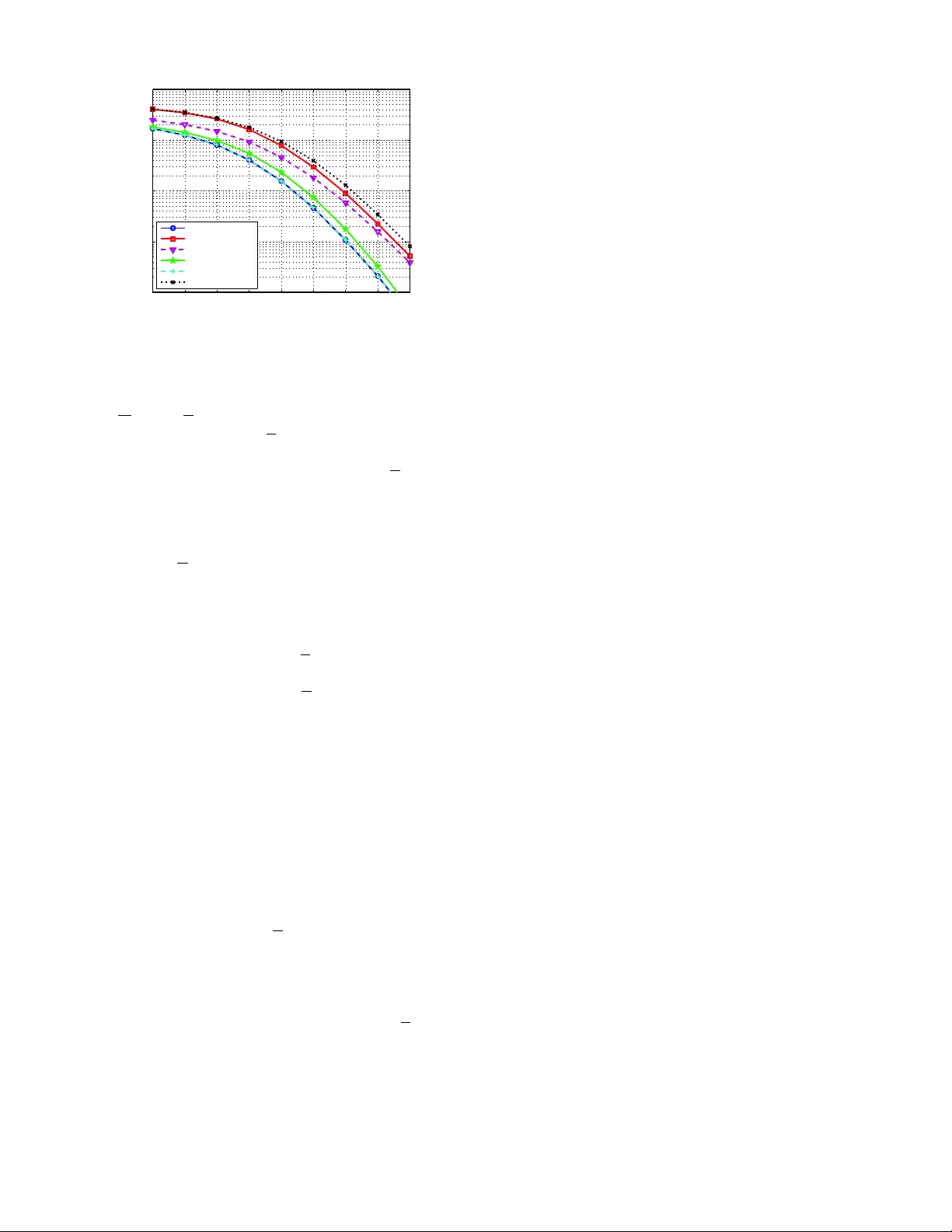
1 Finite Lattice-Size Ef fects in MIMO Detection C. Studer ∗ , D. Seethaler ‡ , and H. Bölcskei ‡ ∗ Integrated Systems Laboratory ETH Zurich, 8092 Zurich, Switzerland e-mail: studer@iis.ee.ethz.ch ‡ Communication T echnology Laboratory ETH Zurich, 8092 Zurich, Switzerland e-mail: {seethal,boelcskei}@nari.ee.ethz.ch Abstract —Many powerful data detection algorithms employ ed in multiple-input multiple-output (MIMO) communication sys- tems, such as sphere decoding (SD) and lattice-reduction (LR)- aided detection, were initially designed for infinite lattices. Detec- tion in MIMO systems is, however , based on finite lattices. In this paper , we systematically study the consequences of finite lattice- size for the perf ormance and complexity of MIMO detection algorithms formulated for infinite lattices. Specifically , we find, considering perf ormance and complexity , that LR does not seem to offer advantages when used in conjunction with SD. I . I N T RO D U C T I O N The computational complexity associated with maximum- likelihood (ML) detection (MLD) in multiple-input multiple- output (MIMO) communication systems poses significant challenges for corresponding VLSI implementations [1]. Promising approaches for complexity reduction make explicit use of the structure in the problem by transforming it into an equi valent lattice decoding 1 problem, where the underlying lattice is finite. Some of the most prominent techniques for efficient lattice decoding were, howe ver , de veloped for infinite lattices, e.g., sphere decoding (SD) [2] or lattice-reduction (LR)-aided detection, e.g., [3], [4]. The goal of this paper is to in vestigate the fundamental differences, in terms of complexity and performance, between MIMO detection on finite and on infinite lattices. W e sho w that relaxation of the MIMO detection problem to infinite lattices followed by LR can reduce the complexity of SD at the cost of a significant performance loss in terms of error rate. This performance loss is caused by symbol estimates that do not belong to the finite lattice and hence require remapping (onto the finite lattice). W e demonstrate that (near-)ML achieving remapping strategies entail a complexity which is comparable to that of SD operating directly on the finite lattice, thus rendering LR in conjunction with SD unattracti ve for practical applications. Notation: Matrices are set in boldface capital letters, vec- tors in boldface lowercase letters. The superscripts T and H stand for transpose and conjugate transpose, respecti vely . W e write A i,j for the entry in the i th row and j th col- umn of the matrix A , b i for the i th entry of the vec- tor b = [ b 1 b 2 · · · b N ] T , and we denote the ` 2 -norm of b ∈ C N as k b k . I N stands for the N × N identity matrix and This work was supported in part by the STREP project No. IST -026905 (MASCO T) within the Sixth Frame work Programme (FP6) of the European Commission. 1 In the context of this paper it would be more appropriate to use the term “lattice detection”. 1 N denotes the N -dimensional all-ones vector . |O | designates the cardinality of the set O and CZ stands for the set of Gaussian integers, i.e., CZ = Z + √ − 1 Z . The real and imaginary part of x ∈ C is denoted by <{ x } and ={ x } , respectiv ely . I I . M I M O D E T E C T I O N A S L A T T I C E D E C O D I N G Consider a coherent MIMO system, i.e., the recei ver has perfect channel state information (CSI) while the transmitter does not hav e CSI, with M transmit and M receive antennas 2 . The bit-stream to be transmitted is mapped to M -dimensional transmit symbol vectors s ∈ O M , where O corresponds to the underlying scalar QAM constellation. The associated complex baseband input-output relation is giv en by y = Hs + n (1) where H stands for the M × M channel matrix, y is the M - dimensional receiv ed signal vector , and n is an i.i.d. circu- larly symmetric complex Gaussian distributed noise vector of dimension M with v ariance N o per complex entry . The signal- to-noise ratio is defined as SNR = E s / N o , where E s denotes the average signal power per receive antenna. A. T ransformation to Lattices In order to see that the MIMO detection problem is equiv- alent to a lattice decoding problem, we start by mapping the elements s ∈ O to elements x ∈ CZ using the transforma- tion x = as + c . The constants a, c ∈ R with a > 0 and c > 0 are independent of s and are chosen such that x ∈ X ⊂ CZ with |X | = |O | and X =  x ∈ CZ | ( k min ≤ <{ x } ≤ k max ) ∧ ( k min ≤ ={ x } ≤ k max )  (2) where k min , k max ∈ Z . Note that (2) can be used for square QAM constellations to check whether x 0 ∈ CZ is in X by performing separate boundary checks for the real and imaginary part of x 0 . In the case of non-square QAM constel- lations the boundary checks take a slightly more complicated form. The transmit vectors s ∈ O M can be mapped to vectors x ∈ X M ⊂ ( CZ ) M according to x = a s + c (3) 2 The restriction to the number of transmit antennas being equal to the number of receive antennas is made for simplicity of exposition. The results are also valid for the number of receive antennas being larger than the number of transmit antennas. 2 where c = c 1 M . The in verse transformation associated with (3) is giv en by s = a − 1 ( x − c ) . The input-output relation (1) can now be transformed into r = Gx + n (4) where G = a − 1 H and r = y + Gc is a translated version of the received vector y . The essence of the transformation of (1) into (4) is that no w the receiv ed vector r can be interpreted as a lattice point u ∈ L ( G ) that has been translated by the additiv e Gaussian noise vector n . Here, L ( G ) , n Gx | x ∈ X M o (5) denotes the finite lattice generated by G . In the remainder of the paper , we shall work with the input-output relation (4) exclusi vely . B. ML Detection MLD in MIMO systems computes the estimate ˆ u ML = D ML ( r ) = arg min u ∈L ( G ) k r − u k (6) which amounts to solving a closest-vector problem (CVP) in the finite lattice L ( G ) . Since each lattice point in L ( G ) is associated with a transmit vector in X M according to the re- lation u = Gx , the ML-estimate ˆ u ML obtained by solving (6) can be transformed into 3 ˆ x ML = G − 1 ˆ u ML , which upon in ver - sion of (3) yields the ML-estimate ˆ s ML . Solving (6) through an exhausti ve search over all lattice points in L ( G ) typically results in high computational complexity as |L ( G ) | = |X | M may be large. C. Relaxation and Lattice Reduction A promising approach to reducing the computational com- plexity associated with solving (6) is to relax the finite lattice in (5) to the infinite lattice 4 L ( G ) , n Gx | x ∈ ( CZ ) M o (7) and to solve a relaxed version of (6) by computing ˆ u ML = D ML ( r ) = arg min u ∈L ( G ) k r − u k (8) i.e., by searching over the infinite lattice generated by G . This search can be carried out more efficiently by using algorithms from lattice theory , e.g., SD [2] possibly in conjunction with LR through the LLL algorithm [5]. As the resulting esti- mate ˆ u ML is not necessarily in L ( G ) , remapping of ˆ u ML onto the finite lattice L ( G ) is required whenev er ˆ u ML / ∈ L ( G ) . In the remainder of the paper, the term “MLD” always refers to the finite-lattice MLD problem (6), whereas “relaxed MLD” is used to refer to the infinite-lattice MLD problem (8). 3 Note that we implicitly assume that G has full rank; this is satisfied, for example, with probability 1, if the entries of G are i.i.d. circularly symmetric complex Gaussian distributed. Furthermore, in practice G − 1 does not have to be computed explicitly as u in (6) can be replaced by Gx and the minimization can be performed over x ∈ X M . 4 In the remainder of the paper, underlined quantities always refer to the infinite-lattice case. The main motiv ation for relaxation resides in the fact that LR can be applied only to infinite lattices. LR computes an equiv alent and “more orthogonal” basis (for the lattice L ( G ) ) with the generator matrix B = GT , where T is an M × M unimodular matrix, i.e., | det( T ) | = 1 with T i,j ∈ CZ ( ∀ i, j ). Thanks to the unimodularity of T , we hav e L ( B ) = L ( G ) . It is important to note that this equiv alence holds only for infinite lattices, in contrast to finite lattices where L ( B ) 6 = L ( G ) , in general. W e therefore conclude that relaxation to an infinite lattice is essential for the application of LR to MIMO detec- tion. W e emphasize that LR, in general, reduces the complexity of a subsequent SD step and results in (often significant) performance improvements when follo wed by sub-optimal detectors. In particular, in [6] it is shown that LR followed by linear detection achiev es full diversity . D. Schnorr-Euc hner Sphere Decoding SD was initially designed for the efficient solution of CVPs on infinite lattices [2], but has also prov en very efficient for MLD [7], [8]. In the follo wing, we briefly revie w the main ingredients of Schnorr-Euchner SD (SESD) with radius reduction for the finite-lattice case [9]. The algorithm starts by performing a QR decomposition (QRD) of G according to G = QR , where the M × M matrix Q is unitary and the upper-triangular M × M matrix R has real-v alued non-ne gati ve entries on its main diagonal. Left- multiplying (4) by Q H leads to the modified input-output relation ˜ r = Rx + ˜ n , where ˜ r = Q H r and ˜ n = Q H n is again (thanks to Q being unitary) i.i.d. circularly sym- metric complex Gaussian distributed with variance N o per complex entry . W e arrange the partial symbol vectors (PSVs) x ( i ) = [ x i x i +1 · · · x M ] T in a tree that has its root just abo ve lev el i = M and leaves on level i = 1 ; the leaves correspond to vectors x ∈ X M . Each PSV is associated with a partial distance (PD) according to d  x ( i )  =   ˜ r ( i ) − R i x ( i )   , i = 1 , 2 , . . . , M (9) where ˜ r ( i ) = [ ˜ r i ˜ r i +1 · · · ˜ r M ] T and R i contains the lower - right ( M − i + 1) × ( M − i + 1) -dimensional sub-block of R . The MLD problem has therefore been transformed into a weighted tree-search problem, where PSVs and PDs are associated with nodes in the tree. For brevity , we shall often say “the node x ( i ) ” meaning the node corresponding to the PSV x ( i ) . Each path through the tree (from the root node do wn to a leaf node) corresponds to a symbol vector x ∈ X M . Note that in the infinite-lattice case, the tree-search problem needs to be relaxed to vectors x ∈ ( CZ ) M . The solution of (6) is giv en by the leaf associated with the smallest metric. The essence of SD is to constrain the search in the tree through a sphere constraint (SC), realized by searching only those nodes that satisfy d  x ( i )  ≤ r , where r is the search radius associated with a hypersphere centered in the received point. SESD refers to conducting the tree search in a depth- first manner and visiting the children of a given node in ascending order of their PDs [9]. Since the PDs d  x ( i )  are non-decreasing as a function of i = M , M − 1 , . . . , 1 , a node x ( i ) violating the SC can be pruned along with 3 the entire subtree emanating from that node. The algorithm initializes r = ∞ and performs the update r ← d ( x ) whene ver a valid leaf node x has been found. This approach is known in the literature as radius reduction [1], [9]. The complexity measure emplo yed in this paper is giv en by the number of nodes visited by SESD in the tree search, including the leaf nodes, b ut excluding the root node. This complexity measure is directly related to the VLSI imple- mentation complexity for the finite-lattice case 5 [1]. The complexity required for preprocessing (i.e., QRD or LR) will be ignored throughout the paper . W e note, howe ver , that in latency-critical applications, the preprocessing comple xity can be critical. In the remainder of the paper, “SESD”, “relaxed SESD”, and “LR-aided SESD” refer to SESD on finite lattices, on infinite lattices, and to LR followed by SESD on infinite lattices, respectively . I I I . C O M P L E X I T Y O F S E S D A N D O F R E L A X E D S E S D W e next analyze the differences in the complexity behavior of SESD and of relaxed SESD. A. Low-SNR Re gime F inite-lattice case: SESD visits a node x ( i ) if the SC d  x ( i )  ≤ r is satisfied. Since the minimum search radius of SESD (guaranteeing that the corresponding hypersphere contains at least one lattice point) is giv en by the Euclidean distance between the received vector and the ML solution, we can conclude that SESD visits at least all nodes x ( i ) satisfying d  x ( i )  ≤ min x ∈X M k ˜ r − Rx k = r min . (10) Thanks to radius reduction, the final (with respect to the repeated tree-trav ersals as described abov e) search radius of SESD corresponds to r min . W e can therefore conclude that the genie-aided choice r = r min for the search radius initialization, indeed, yields a lower bound on the number of nodes visited by SESD. Denoting the transmitted data vector as x 0 ∈ X M , we obtain a lower bound on r min as follows: r min a ) = min x ∈X M   ˜ n + R ( x 0 − x )   ≥ b) ≥ min x ∈X M  k ˜ n k −   R ( x − x 0 )    = = k ˜ n k − max x ∈X M   R ( x − x 0 )   ≥ c) ≥ k ˜ n k − σ max ( R ) K (11) where a) results from ˜ r = Rx 0 + ˜ n , b) follows from the in verse triangle inequality , and c) is a consequence of the Rayleigh-Ritz theorem [10] ( σ max ( R ) denotes the largest singular value of R ) and the fact that the con- stant K = max x , x 0 ∈X M k x − x 0 k is finite in the finite-lattice case. From (11) we can infer that SESD visits at least all nodes x ( i ) satisfying d  x ( i )  ≤ k ˜ n k − σ max ( R ) K. (12) 5 W e expect this complexity measure to be equally relev ant for the infinite- lattice case. Note that setting the search radius equal to the right-hand side (RHS) of (12) will no longer guarantee that the correspond- ing hypersphere contains at least one lattice point. This is, howe ver , irrelev ant for the point we want to make next. Defining v = ˜ n / √ N o , we can rewrite (12) as      v ( i ) + R i  x 0 ( i ) − x ( i )  √ N o      ≤ k v k − σ max ( R ) K √ N o . (13) W e can now see that for N o → ∞ and hence for SNR → 0 , the condition in (13) reduces to   v ( i )   ≤ k v k , which is trivially satisfied for i > 1 for ev ery realization of ˜ n and for gi ven R . In this case, SESD visits at least all nodes down to and including the le vel just above the leaf lev el. An intuitiv e explanation for this effect is that the noise can shift the transmit vector arbitrarily far aw ay from the finite lattice and hence, the RHS of (11) and consequently r min can become arbitrarily large, which inhibits efficient tree pruning. Infinite-lattice case: The fundamental dif ference between the complexity of SESD and of relaxed SESD is due to the fact that in the infinite-lattice case, the maximum distance between the recei ved vector r and the nearest lattice point is bounded for a given (full rank) R . The complexity of relaxed SESD can therefore be lower than that of SESD. The downside is that relaxed SESD is not guaranteed to find the ML solution, which necessarily has to be a point in the finite lattice L ( G ) . Specifically , if relaxed SESD delivers a lattice point outside L ( G ) , this point needs to be remapped onto the finite lattice. Corresponding remapping approaches are described in Section IV. In the following, we derive an analytic upper bound on the complexity of relaxed SESD. The number of nodes x ( i ) on tree lev el i that satisfy the SC with radius r is denoted by C i ( r ) and corresponds to the number of lattice points in L ( R i ) that are within a 2( M − i + 1) -dimensional (real-valued) hypersphere of radius r centered at r ( i ) . This number can be upper-bounded by dividing the volume of a 2( M − i + 1) -dimensional hypersphere of radius r + µ i by the volume of a V oronoi cell in L ( R i ) [11], where µ i corresponds to the covering radius of the lattice L ( R i ) [12]. More specifically , we have [13] C i ( r ) ≤ V ( M − i +1) ( r + µ i ) V ol  L ( R i )  (14) where V k ( r ) = π k k ! r 2 k denotes the volume of a 2 k -dimensional hypersphere with radius r and the volume of a V oronoi cell of L ( R i ) is V ol  L ( R i )  = det( R H i R i ) . In order to derive an upper bound on the total complexity C = P M i =1 C i ( r ) of relaxed SESD, we consider the case where only the first radius update is performed. The first leaf node found by relaxed SESD corresponds to the Babai point ˆ x B [14] and hence the radius after the first update from the initial value r = ∞ is giv en by d  ˆ x B  , which can be upper-bounded as [9], [14] d  ˆ x B  =   ˜ r − R ˆ x B   ≤ v u u t 1 2 M X j =1 R 2 j,j = β . (15) Since the covering radius µ 1 is also upper-bounded by β [11], [15] and, more generally , µ i can be upper-bounded 4 as µ i ≤ q 1 2 P M j = i R 2 j,j = γ i , we have r + µ i ≤ β + γ i , which yields an upper bound on the total complexity of relaxed SESD according to C ≤ M X i =1 V ( M − i +1) ( β + γ i ) det( R H i R i ) . (16) B. High-SNR Re gime In the high-SNR regime, relaxed SESD is likely to return the ML solution. Moreov er , if k ˜ n k is sufficiently small, relaxed SESD and SESD find the same leaf nodes, which will belong to the finite lattice L ( G ) . Consequently , relaxed SESD and SESD will operate with the same search radii and hence the same SCs. Howe ver , the tw o detectors will, in general, not exhibit the same complexity , as the SESD additionally (to the SC) takes into account the finite alphabet nature of X ⊂ CZ , whereas relaxed SESD visits all points in CZ satisfying the SC. Therefore, in the high-SNR regime, SESD tends to result in smaller complexity than relaxed SESD. C. Numerical Complexity Assessment A simple numerical result serves to demonstrate the poten- tial complexity savings of relaxed SESD over SESD in the low-SNR regime. W e assume a MIMO channel with R = I M and M = 4 . Counting all the nodes do wn to and including the lev el just abov e the leaf lev el and noting that only one leaf node is visited by SESD if R is a diagonal matrix, leads to the corresponding complexity C = |X | M − 1 |X | − 1 of SESD for SNR → 0 (see the discussion in the last paragraph of Section III-A). For a 16-QAM alphabet, this leads to C = 4369 nodes. The total complexity of relaxed SESD is upper-bounded by (16), which can be refined by noting that relaxed SESD visits only one leaf node in the case of R = I M . Consequently , we hav e C ≤ 1 + M X i =2 V ( M − i +1) r M 2 + r M − i + 1 2 ! which sho ws that at most 1928 nodes will be visited, irrespec- tiv ely of the SNR. W e can therefore conclude that relaxation can result in a significant complexity reduction at low SNR values. Fig. 1 shows the complexity 6 corresponding to SESD (which yields ML performance) and to relaxed SESD (de- noted by R-SESD). Consistent with the observations made in Sections III-A and III-B, we see that relaxation leads to com- plexity savings in the low-SNR regime, but results in higher complexity in the high-SNR regime. W e can furthermore see 6 All simulation results are for an uncoded M = 4 MIMO system with 16-QAM symbol constellation using Gray labeling. The entries of H are i.i.d. circularly symmetric complex Gaussian distributed with unit variance. For (relaxed) SESD, we use sorted QR-decomposition (SQRD) according to [16], for LR, a complex-valued variant of the LLL algorithm with δ = 3 / 4 and SQRD preprocessing as described in [17], [18]. All complexity and performance simulations are averaged over 640,000 channel realizations and for each channel realization a single noise realization has been generated. that relaxation follo wed by LR (denoted by LR-SESD) leads to lower complexity than SESD for all SNR values. The complexity reductions of R-SESD and LR-SESD over SESD come, ho wev er, at a significant performance loss in terms of error-rate and in the case of LR-SESD also at increased computational complexity in the preprocessing stage caused by the need for LR (realized through the LLL al- gorithm [5], for example). For naiv e lattice decoding, i.e., estimates ˆ u ML / ∈ L ( G ) are simply discarded and an error is declared, Fig. 2 shows a 3 dB SNR loss of LR-SESD com- pared to SESD (MLD). W e emphasize that the performance of R-SESD, not shown in Fig. 2, is identical to that of LR-SESD; the associated complexities are, ho wever , different (cf. Fig. 1). Note that naiv e lattice decoding was shown to achie ve full div ersity , while leading to an unbounded SNR gap (growing logarithmically in SNR) for MIMO systems with an equal number of transmit and receiv e antennas [19]. In the next section, we discuss sev eral approaches to the mitigation of this performance loss, i.e., we consider algorithms for remapping estimates ˆ u ML / ∈ L ( G ) onto L ( G ) . I V . R E M A P P I N G M E T H O D S If the estimate deli vered by relaxed SESD satisfies ˆ u ML ∈ L ( G ) , the lattice point ˆ u ML corresponds to the ML solution (6), i.e., ˆ u ML = ˆ u ML . If ˆ u ML / ∈ L ( G ) and the performance of naive lattice decoding is not sufficient, the solution deli vered by relaxed SESD needs to be remapped onto the finite lattice L ( G ) . Since all constellation points x ∈ X M (corresponding to elements u ∈ L ( G ) through the relation 7 u = Gx ) satisfy (2), determining whether ˆ u ML is in the finite lattice L ( G ) can be performed efficiently through element- wise boundary checks of the real and imaginary parts of ˆ x ML . In the following, we briefly revie w an existing remapping method known as quantization and describe novel remap- ping approaches that realize different performance/comple xity trade-offs. A. Quantization The standard remapping approach known in the literature is quantization and amounts to remapping ˆ x ML / ∈ X M to the closest (in Euclidean distance) symbol vector ˆ x q ∈ X M according to [4], [18] ˆ x q = arg min x ∈X M   ˆ x ML − x   . (17) As quantization corresponds to element-wise slicing of the entries of ˆ x ML to the nearest candidates in X , it requires low computational comple xity . The resulting estimate ˆ x q does, howe ver , not necessarily correspond to the ML solution (6) and hence leads to a (potentially significant) performance loss. Fig. 2 shows the performance obtained by LR-aided SESD followed by remapping through quantization (denoted by LR-SESD, quant.). The numerical results indicate a slight improv ement ov er naive lattice decoding, but still show a 7 In the remainder of the paper , we treat v ectors x ∈ ( CZ ) M and u ∈ L ( G ) as well as x ∈ X M and u ∈ L ( G ) as interchangeable as they are related through the one-to-one mappings u = Gx and u = Gx , respectively . Of course, this assumes that G has full rank. 5 2.5 dB SNR loss compared to ML performance. Finally , Fig. 2 shows the performance obtained by LR-aided successi ve interference cancellation (SIC) on the infinite lattice with remapping through naiv e lattice decoding (denoted by LR-SIC, naiv e). The resulting performance loss, compared to relaxed SESD with remapping through naiv e lattice decoding, is low (approximately 0.25 dB SNR), whereas the complexity of LR- SIC is significantly lower than that of LR-SESD. B. Optimal Lattice Remapping The discussion abov e brings out the importance of remap- ping. It is therefore natural to ask for the optimum lattice remapping strategy in the sense of maximizing the probability of the result of remapping to correspond to the transmitted symbol vector giv en the result of the relaxed detector ˆ u . Let u 0 ∈ L ( G ) be the transmitted vector and assume that the relaxed detector yields D ( r ) = D ( u 0 + n ) = ˆ u , ˆ u ∈ L ( G ) \ L ( G ) . Optimal lattice remapping according to the criterion described abov e now amounts to identifying the lattice point u ∈ L ( G ) which maximizes P[ u 0 = u | D ( r ) = ˆ u ] , i.e., ˆ u opt = arg max u ∈L ( G ) P[ u 0 = u | D ( r ) = ˆ u ] . W e emphasize that the optimum remapping rule depends on D ( r ) and hence, on the relaxed MIMO detector employed. Using Bayes’ s theorem and assuming that all transmit vectors are equally likely , we get ˆ u opt = arg max u ∈L ( G ) P[ D ( r ) = ˆ u | u 0 = u ] (18) which amounts to solving a finite-lattice MLD problem (6) based on the relaxed estimate ˆ u instead of the receiv ed vec- tor r . W e stress that relax ed MLD followed by optimum lattice remapping according to (18) will, in general, not achiev e ML performance as remapping is conducted based on ˆ u rather than on r . F or the sake of simplicity of exposition, in the following, we write P[ D ( r ) = ˆ u | u ] instead of P[ D ( r ) = ˆ u | u 0 = u ] . Closest-vector r emapping: The optimal remapping rule in (18) can, in general, not be expressed in closed form, as it depends on the decision region of the relaxed MIMO detector . W e can, howe ver , obtain a simple remapping strategy that achiev es near-optimal performance by computing an approxi- mation of (18) as follows. W e start by noting that P[ D ( r ) = ˆ u | u ] = Z D ( ˆ u ) f G ( w − u ) d w (19) where f G ( w ) = ( π N o ) − M exp  − N − 1 o k w k 2  is the joint probability density function of a multi-variate complex Gaussian with i.i.d. circularly symmetric components each of which has variance N o and D ( ˆ u ) = n w ∈ C M | D ( w ) = ˆ u o denotes the decision region of the relaxed MIMO detector employed. Next, we consider optimal remapping for relaxed 10 12 14 16 18 20 22 24 26 0 5 10 15 20 25 30 SNR [dB] Complexity SESD (MLD) R-SESD LR-SESD LR-SESD, CVR LR-SESD, MLD Fig. 1. Complexity of SESD (MLD), relaxed SESD (R-SESD), and LR-aided SESD (LR-SESD). MLD, i.e., D ( r ) = D ML ( r ) as defined in (8) and ˆ u = ˆ u ML , and note that in this case (19) formally corresponds to the probability of mistakenly decoding the transmitted point u for ˆ u ML . This probability can be upper-bounded as P h D ML ( r ) = ˆ u ML   u i ≤ Q   ˆ u ML − u   √ 2 N o ! (20) where Q ( a ) = (2 π ) − 1 2 R ∞ a exp( − x 2 2 ) d x . Replacing the func- tion to be maximized ov er in (18) by the upper bound in (20) leads to a nov el remapping rule, which we refer to as closest- vector remapping (CVR) and which is giv en by ˆ u cv = arg min u ∈L ( G )   ˆ u ML − u   . (21) The solution of (21) corresponds to the point ˆ u cv ∈ L ( G ) that is closest (in Euclidean distance) to the lattice point ˆ u ML ∈ L ( G ) \ L ( G ) . W e emphasize that CVR amounts to solving a finite-lattice CVP and can, hence, be carried out by (non- relaxed) SESD with the relaxed ML-estimate ˆ u ML taking the role of the receiv ed point. Note that CVR according to (21) ex- hibits structural similarities to quantization according to (17). Formally , quantization can be seen as CVR with G = I M , which amounts to ignoring the structure of the lattice generated by G . Numerical performance and complexity r esults: Fig. 2 com- pares the performance of relaxed SESD followed by CVR to that obtained by relaxed SESD followed by quantization. W e observe that CVR significantly outperforms quantization (and naiv e lattice decoding) and yields close-to-ML performance. This improvement comes, howe ver , at the cost of having to solve a finite-lattice CVP , namely (21), in contrast to simple element-wise slicing in the case of quantization and to simply discarding estimates that do not belong to L ( G ) in the case of naiv e lattice decoding, both of which exhibit significantly smaller complexity . W e next compare the overall complexity (i.e., the total complexity of both SESD runs) of LR-aided SESD followed by CVR (denoted by LR-SESD, CVR) to that of SESD op- erating directly on the finite lattice, i.e., SESD (MLD). Fig. 1 shows that LR-SESD with CVR outperforms SESD (MLD) only in the very-high-SNR regime with the corresponding complexity savings being minor . In addition, this comparison fa vors LR-SESD with CVR as the additional complexity associated with LR has been neglected. 6 10 12 14 16 18 20 22 24 26 10 -4 10 -3 10 -2 10 -1 10 0 SNR [dB] BER SESD (MLD) LR-SESD, naive LR-SESD, quant. LR-SESD, CVR LR-SESD, MLD LR-SIC, naive Fig. 2. Bit error rate (BER) performance comparison of SESD (MLD), LR-SESD, and LR-SIC. C. T wo-Stage Detection The discussion abov e leads us to the question of whether using D ( r ) = ˆ u for remapping instead of r is sensible. After all, by mapping r onto ˆ u we are potentially discarding useful information. In the follo wing, we show that, indeed, performing remapping based on r rather than on ˆ u leads to a performance improvement (compared to, e.g., CVR) without requiring additional complexity . T o this end, we propose a new detector structure, which consists of two stages. The first stage corresponds to relaxation from L ( G ) to L ( G ) (possibly followed by LR) and using a relaxed MIMO detector . The second stage is inv oked only if the first stage yields a result that does not belong to the finite lattice L ( G ) and corresponds to a MIMO detector operating on the finite lattice. This second-stage detector uses the received vector r instead of ˆ u . W e emphasize that if both stages employ MLD, the tw o-stage detector achie ves ML performance, since in the case of ˆ u ML / ∈ L ( G ) , the second stage performs non-relaxed MLD on the basis of r . Numerical performance and complexity r esults: Fig. 1 shows the overall complexity of two-stage detection (i.e., the total complexity across the two stages) using LR-aided SESD in the first stage and SESD in the second stage (denoted by LR-SESD, MLD). Again, the complexity associated with LR is ignored. Consulting the corresponding performance results in Fig. 2, we can conclude that two-stage detection employing SESD in both stages and LR in the first stage outperforms LR-SESD with CVR both in terms of complexity and per- formance and, hence, the performance loss associated with LR-SESD followed by CVR (compared to ML performance) must result from the fact that ˆ u ML rather than r is used for remapping. W e can furthermore conclude that in the high- SNR re gime the two-stage approach e xhibits slightly lower complexity than SESD, while realizing the same (i.e., ML) performance. W e finally note that the computational complex- ity of LR and the complexity of checking whether ˆ u ∈ L ( G ) has been neglected in this comparison. V . C O N C L U S I O N S W e demonstrated that relaxation from finite to infinite lattices combined with lattice reduction (LR) can reduce the (tree-search) complexity of Schnorr-Euchner sphere decoding (SESD), but generally leads to a significant performance loss. This performance loss is caused by the fact that the relaxed detector does not necessarily deliv er estimates that belong to the finite lattice and hence does not realize ML performance. Remapping methods that yield (close-to) ML performance ne- cessitate solving finite-lattice closest vector problems (CVPs). Hence, if ML performance is required, using SESD directly on the finite lattice seems to require smaller complexity , as remapping is av oided and only one (finite-lattice) CVP needs to be solved. W e proposed an ML-optimal two-stage detector which was shown to require lower complexity than SESD on the finite lattice provided i) the SNR is high enough and ii) the complexity corresponding to LR and to checking whether estimates correspond to the finite lattice is ne glected. Generally speaking, we conclude that relaxation and LR are better suited for use in conjunction with lo w-complexity detectors (such as linear detection or SIC) with overall sub-optimal performance. R E F E R E N C E S [1] A. Burg, M. Borgmann, M. W enk, M. Zellweger , W . Fichtner, and H. Bölcskei, “VLSI implementation of MIMO detection using the sphere decoding algorithm, ” IEEE J ournal of Solid-State Cir cuits , vol. 40, no. 7, pp. 1566–1577, July 2005. [2] U. Fincke and M. Pohst, “Improved methods for calculating vectors of short length in a lattice, including a complexity analysis, ” Math. of Computation , v ol. 44, pp. 463–471, Apr . 1985. [3] H. Y ao and G. W ornell, “Lattice-reduction-aided detectors for MIMO communication systems, ” in Proc. IEEE GLOBECOM , vol. 1, Nov . 2002, pp. 424–428. [4] C. W indpassinger and R. F . H. Fischer , “Low-complexity near- maximum-likelihood detection and precoding for MIMO systems using lattice reduction, ” in Pr oc. IEEE Inf . Theory W orkshop , Mar . 2003, pp. 345–348. [5] A. K. Lenstra, H. W . Lenstra, and L. Lovász, “Factoring polynomials with rational coefficients, ” Mathematische Annalen , vol. 261, no. 4, pp. 515–534, Dec. 1982. [6] M. T aherzadeh, A. Mobasher, and A. K. Khandani, “LLL reduction achiev es the receive div ersity in MIMO decoding, ” IEEE T rans. on Inf. Theory , v ol. 53, no. 12, pp. 4801–4805, Dec. 2007. [7] W . H. Mow , “Maximum likelihood sequence estimation from the lattice viewpoint, ” Master’ s thesis, Chinese University of Hong K ong, Dept. of Information Engineering, June 1991. [8] E. V iterbo and E. Biglieri, “ A univ ersal decoding algorithm for lattice codes, ” Colloque sur le T raitement du Signal et ses Applications (GRETSI) , v ol. 14, pp. 611–614, Sept. 1993. [9] E. Agrell, T . Eriksson, A. V ardy , and K. Zeger, “Closest point search in lattices, ” IEEE Tr ans. on Inf. Theory , vol. 48, no. 8, pp. 2201–2214, Aug. 2002. [10] R. A. Horn and C. R. Johnson, Matrix Analysis . Cambridge Univ . Press, 1985. [11] A. H. Banihashemi and A. K. Khandani, “On the complexity of decoding lattices using the Korkin-Zolotare v reduced basis, ” IEEE Tr ans. on Inf. Theory , v ol. 44, no. 1, pp. 162–171, Jan. 1998. [12] J. H. Conway and N. J. A. Sloane, Spher e P ackings, Lattices and Gr oups , 3rd ed. Springer , 1999. [13] J. M. W ills, “Bounds for the lattice point enumerator, ” Geometriae Dedicata , v ol. 40, no. 2, pp. 237–244, No v . 1991. [14] L. Babai, “On Lovász’ lattice reduction and the nearest lattice point problem, ” Combinatorica , vol. 6, no. 1, pp. 1–13, Mar. 1986. [15] R. Kannan, “Minkowski’ s con ve x body theorem and integer program- ming, ” Math. of Operations Researc h , vol. 12, no. 3, pp. 415–440, Aug. 1987. [16] D. Wübben, R. Böhnke, J. Rinas, V . Kühn, and K.-D. Kammeyer, “Effi- cient algorithm for decoding layered space-time codes, ” IEE Electr onics Letters , vol. 37, no. 22, pp. 1348–1350, Oct. 2001. [17] Y . H. Gan and W . H. Mow , “Complex lattice reduction algorithms for low-comple xity MIMO detection, ” in Pr oc. IEEE GLOBECOM , Nov . 2005, pp. 2953–2957. [18] D. Wübben, R. Böhnke, V . Kühn, and K.-D. Kammeyer , “MMSE-based lattice-reduction for near-ML detection of MIMO systems, ” in Pr oc. ITG/IEEE W orkshop on Smart Antennas , Mar. 2004, pp. 106–113. [19] M. T aherzadeh and A. K. Mahmoud, “On the limitations of the naiv e lattice decoding, ” in Pr oc. IEEE Int. Symp. on Inf. Theory , June 2007, pp. 201–204.