A congruence problem for polyhedra

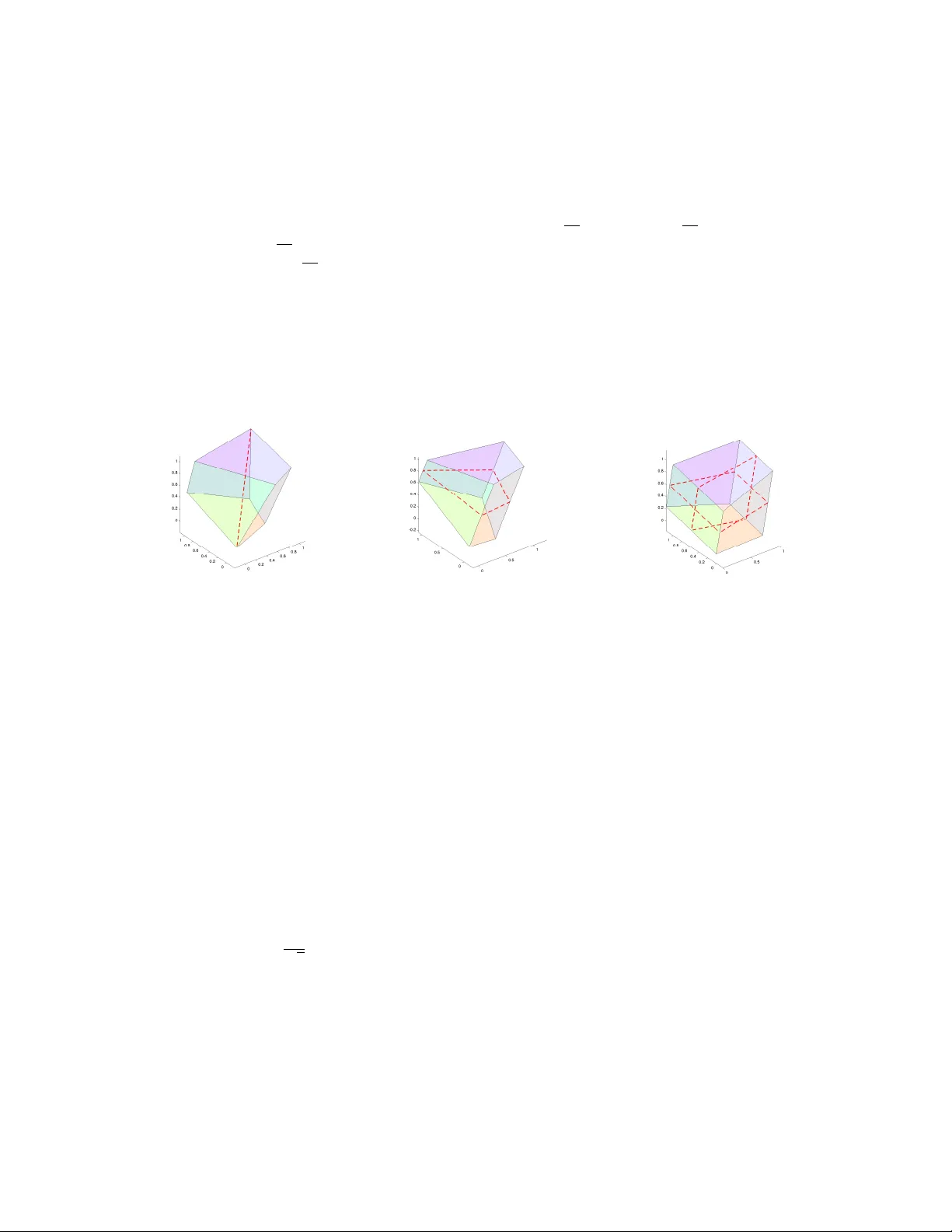
A congruence problem for p olyhedra Alexander Boriso v, Mark Dic kinson, Stuart Hastings Octob er 25, 2018 Abstract It is w ell known that to determine a triangle up to congruence requires three measuremen ts: three sides, t wo sides and the included angle, or one side and t wo angles. W e consider v arious generalizations of this fact to tw o and three dimensions. In particular w e consider the follo wing question: given a con vex p olyhedron P , how many measurements are required to determine P up to congruence? W e sho w that in general the answer is that the num b er of measurements required is equal to the n umber of edges of the p olyhedron. Ho wev er, for many p olyhedra few er measurements suﬃce; in the case of the unit cub e we show that nine carefully chosen measurements are enough. W e also prov e a num b er of analogous results for planar p olygons. In particular we describ e a v ariet y of quadrilaterals, including all rhombi and all rectangles, that can b e determined up to congruence with only four measuremen ts, and w e prov e the existence of n -gons requiring only n measurements. Finally , w e show that one cannot do better: for an y sequence of n distinct points in the plane one needs at least n measuremen ts to determine it up to congruence. 1 In tro duction W e discuss a class of problems ab out the congruence or similarity of three dimensional p olyhedra. The basic format is the following: Problem 1.1. Giv en tw o p olyhedra in R 3 whic h hav e the same combinatorial structure (e.g. b oth are hexahedra with four-sided faces), determine whether a given set of measuremen ts is suﬃcient to ensure that the p olyhedra are congruent or similar. W e will make this more sp eciﬁc b y sp ecifying what sorts of measuremen ts will b e allow ed. F or example, in muc h of the pap er, allo wed measurements will include distances b et w een pairs of vertices, angles b etw een edges, angles b et w een t w o intersecting face diagonals (possibly on diﬀeren t faces with a common v ertex) or b et w een a face diagonal and an e dge, and dihedral angles (that is, angles b etw een tw o adjoining faces). One motiv ation for these choices is given b elo w. Sometimes we are more restrictive, for example, allowing only distance measurements. In tw o dimensions this w as a fundamental question answered b y Euclidean geometers, as (we hop e) ev ery studen t who takes geometry in high sc ho ol learns. If the lengths of the corresp onding sides of tw o triangles are equal, then the triangles are congruen t. The SAS, ASA, and AAS theorems are equally well known. The extension to other shap es is not often discussed, but we will hav e some remarks ab out the planar problem as w ell. It is surprising to us that b ey ond the famous theorem of Cauch y discussed b elo w, we hav e b een unable to ﬁnd m uc h discussion of the problems we consider in the literature, though w e think it is almost certain that they hav e been studied in the past. W e w ould b e appreciative if any reader can p oin t us to relev an t results. Our approach will usually b e to look at the problem lo cally . If the tw o p olyhedra are almost congruent, and agree in a certain set of measuremen ts, are they congruen t? A t ﬁrst glance this looks like a basic question in what is known as rigidity theory , but a little thought shows that it is diﬀerent. In rigidity theory , atten tion is paid to relativ e p ositions of vertices, viewing these as connected by inextensible ro ds whic h are hinged at their ends and so can rotate relativ e to eac h other, sub ject to constraints imp osed b y 1 the ov erall structure of rods. In our problem there is the additional constraint that in an y mov emen t of the v ertices, the com binatorial structure of the p olyhedron cannot change. In particular, an y vertices that were coplanar b efore the mov emen t must b e coplanar after the mo v ement. This feature seems to us to pro duce an interesting area of study . Our original motiv ation for considering this problem came from a v ery practical question encoun tered b y one of us (SPH). If one attempts to mak e solid w o oden mo dels of interesting polyhedra, using standard w o odworking equipmen t, it is natural to wan t to chec k ho w accurate these mo dels are. 1 As a mathematician one ma y b e attracted ﬁrst to the Platonic solids, and of these, the simplest to make app ears to b e the cub e. (The regular tetrahedron lo oks harder, b ecause non-right angles seem harder to cut accurately . ) It is p ossible to purchase lengths of w oo d with a square cross section, called “turning squares” b ecause they are mostly used in lathes. T o mak e a cub e, all one has to do is use a saw to cut oﬀ the correct length piece from a turning square. Of course, one has to do so in a plane p erp endicular to the planes of sides of the turning square. It is obvious that there are sev eral degrees of freedom, meaning sev eral w a ys to go wrong. The piece cut oﬀ could b e the wrong length, or y ou could cut at the wrong angle, or p erhaps the cross section w asn’t square to begin with. So, y ou start measuring to see how well you hav e done. In this measuremen t, though, it seems reasonable to mak e some assumptions. The basic one of interest here is that the saw cuts oﬀ a planar slice. Y ou also assume that this was true at the sawmill where the turning square w as made. So you assume that you ha v e a hexahedron – a p olyhedron with six faces, all of whic h are quadrilaterals. Do y ou hav e a cube? At this p oint you are not asking a question addressed b y standard rigidity theory . One’s ﬁrst impulse ma y b e to measure all of the edges of the hexahedron, with the thought that if these are equal, then it is indeed a cub e. This is quic kly seen to b e false, b ecause the faces could b e rhom bi. Another intriguing p ossibility that we considered early on is that measuring the tw elv e face diagonals might suﬃce. How ev er, we found some examples showing that this w as not the case, and David Allwright [ 2 ] ga v e a short and elegant quaternion-based classiﬁcation of all hexahedra with equal face diagonals. See also an earlier discussion of this problem in [ 13 ]. 2 Clearly some other conﬁguration of measurements, p erhaps including angles, is necessary . It did not take long to come up with several sets of 12 measuremen ts which did the job, but a pro of that this n um b er was necessary eluded us. In our exp erience most p eople, ev en most mathematicians, who are presen ted with this problem do not see an answ er immediately . Apparently the cube is harder than it lo oks, and so one w ould lik e a simpler problem to get some clues. The (regular) tetrahedron comes to mind, and so one asks how many measuremen ts are required to establish that a p olyhedron with four triangular faces is a tetrahedron. No w w e turn to Cauch y’s theorem. Theorem 1.2 (Cauch y , 1839) . Two c onvex p olyhe dr a with c orr esp onding c ongruent and similarly situate d fac es have e qual c orr esp onding dihe dr al angles. If we measure the six edges of our triangular faced ob ject, and ﬁnd them equal, then we hav e established congruence of the faces of our ob ject to those of a tetrahedron. Cauc hy’s theorem tells us that the dihedral angles are the same and this implies the desired congruence. F or a tetrahedron this result is fairly obvious, but for the t wo other Platonic solids with triangular faces, namely the o ctahedron and the icosahedron, it is less so. Hence Cauc h y’s theorem is of practical v alue to the (extremely ﬁnic ky) woo dw ork er, and shows that for these ob jects, the n um b er of edges is at least an upp er bound on the num b er of measuremen ts necessary to pro ve congruence. F rom now on we will denote the num b er of edges of our p olyhedron b y E , the num ber of v ertices by V and the num ber of faces by F . W e will only consider simply connected p olyhedra, so that Euler’s form ula, V + F = E + 2 , holds. It is not hard to giv e an example showing the necessity of conv exity in Cauch y’s result, but it is one where the tw o polyhedra b eing compared are, in some sense, far apart. It was not easy to determine if conv exity 1 The usual metho d of constructing a p olyhedron is by folding a pap er shell. 2 The face diagonals of a hexahedron are equal when these diagonals form t wo congruent regular tetrahedra whose edges intersect in pairs. As it turns out, this arrangement is not unique. W e hav e included All wrigh t’s analysis of the p ossibilities as Appendix A in the p osting of this pap er to 2 w as necessary for lo cal congruence. Can a nonconv ex polyhedron with all faces triangular b e p erturbed smo othly through a family of noncongruen t p olyhedra while keeping the lengths of all edges constan t? The answ er is yes, as was prov ed in a famous and imp ortan t paper b y R. Connelly in 1979.[ 4 ] Cauc hy’s result also gives us an upp er b ound for the num b er of measurements necessary to determine a unit cube: triangulate the cub e b y dividing eac h square face in to a pair of triangles. Then we ha v e a triangular-faced ob ject with eighteen edges, and b y Cauc h y’s theorem those eigh teen edge measuremen ts suﬃce to determine the cub e up to congruence. Ho wev er, we can do better. Start b y considering a square. W e can approach this algebraically b y assuming that one vertex of the square is at (0 , 0) in the plane. Without loss of generality w e can also take one edge along the x -axis, going from (0 , 0) to ( x 1 , 0) for some x 1 > 0 . The remaining vertices are then ( x 2 , x 3 ) and ( x 4 , x 5 ) and this leads to the conclusion that to determine ﬁve unkno wns, w e need ﬁve equations, and so ﬁv e measurements. F or example, we could measure the four sides of the square and one vertex angle, or we could measure a diagonal instead of the angle. W e then use this to study the cub e. Fiv e measurements show that one face is a square of a sp eciﬁc size. Only four more are needed to sp ecify an adjacent face, because of the common edge, and the three more for one of the faces adjoining the ﬁrst tw o. The requirement that this is a hexahedron then implies that we hav e determined the cub e completely , with tw elv e measurements. This is a satisfying result b ecause it shows that E measuremen ts suﬃce for a cub e as w ell as for the triangular faced Platonic solids. Ho wev er, as remark ed earlier, at this stage w e hav e not prov ed the necessit y of t w elv e measurements, only the suﬃciency . One of the most surprising dev elopments for us in this w ork w as that in fact, t w elve are not necessary . It is p ossible to determine a cub e (including its size) with nine measurements of distances and face angles. The reason, even more surprisingly , is that only four measurements are needed to determine the congruence of a quadrilateral to a sp eciﬁc square, rather than ﬁv e as seemed so obvious in the argument ab o v e. W e will giv e the algorithm that determines a square in four measuremen ts in the ﬁnal section of the paper, whic h con tains a num ber of remarks about congruence of p olygons. F or now, we pro ceed with developing a general metho d for p olyhedra. This metho d will also handle similarit y problems, where the s hape of the p olyhedron is speciﬁed up to a scale change. In determining similarity , only angle measurements are in v olv ed. As the reader migh t exp ect, in general E − 1 measurements suﬃce, with one additional length required to get congruence. 2 E measuremen ts suﬃce In this section w e prov e that for a c onvex p olyhedron P with E edges, there is a set of E measurements that, at least lo cally , suﬃces to determine P up to congruence. W e restrict to conv ex p olyhedra mostly for reasons of con venience: man y of the results b elo w should b e true in greater generalit y . (One problem with moving b ey ond conv ex p olyhedra is determining exactly what the term ‘p olyhedron’ should mean: for a recent attempt to give a general deﬁnition of the term ‘nonconv ex p olyhedron’, see the b eautiful pap er [ 9 ].) T o a void any ambiguit y w e b egin with a precise deﬁnition of conv ex p olyhedron. Deﬁnition 2.1. A close d half-sp ac e is a subset of R 3 of the form { ( x, y , z ) ∈ R 3 | ax + by + cz + d ≥ 0 } with ( a, b, c ) 6 = (0 , 0 , 0). A c onvex p olyhe dr on is a subset P of R 3 whic h is b ounded, do es not lie in any plane, and can b e expressed as an in tersection of ﬁnitely many closed half-spaces. The vertices, edges and faces of a conv ex p olyhedron P can b e deﬁned in terms of intersections of P with suitable closed half-spaces. F or example, a fac e of P is a subset of P of the form P ∩ H for some closed half-space H , suc h that P ∩ H lies entirely within some plane but is not contained in any line. Edges and v ertices can b e deﬁned similarly . The original problem refers to t wo polyhedra with the same ‘combinatorial structure’, so w e giv e a notion of abstr act p olyhe dr on which isolates the combinatorial information embo died in a con v ex p olyhedron. 3 Deﬁnition 2.2. The underlying abstr act p olyhe dr on of a con vex p olyhedron P is the triple ( V P , F P , I P ), where V P is the set of vertices of P , F P is the set of faces of P , and I P ⊂ V P × F P is the incidence relation b et w een vertices and faces; that is, ( v , f ) is in I P if and only if the vertex v lies on the face f . Th us to say that t w o p olyhedra P and Q hav e the same combinatorial structure is to say that their underlying abstract p olyhedra are isomorphic ; that is, there are bijections β V : V P → V Q and β F : F P → F Q that resp ect the incidence relation: ( v , f ) is in I P if and only if ( β V ( v ) , β F ( f )) is in I Q . Note that there is no need to record information ab out the edges; we lea v e it to the reader to verify that the edge data and incidence relations inv olving the edges can b e recov ered from the incidence structure ( V P , F P , I P ). The cardinalit y of the set I P is twice the n um b er of edges of P , since |I P | = X f ∈F P (n umber of vertices on f ) = X f ∈F P (n umber of edges on f ) and the latter sum coun ts eac h edge of P exactly twice. F or the remainder of this section, w e ﬁx a conv ex p olyhedron P and write V , E and F for the num ber of vertices, edges and faces of P , resp ectively . Let Π = ( V , F , I ) b e the underlying abstract p olyhedron. W e are in terested in determining which sets of measuremen ts are suﬃcien t to determine P up to congruence. A natural place to start is with a naiv e dimension coun t: ho w many degrees of freedom does one hav e in sp ecifying a polyhedron with the same combinatorial structure as P ? Deﬁnition 2.3. A r e alization of Π = ( V , F , I ) is a pair of functions ( α V , α F ) where α V : V → R 3 giv es a p oin t for each v in V , α F : F → { planes in R 3 } gives a plane for eac h f in F , and the point α V ( v ) lies on the plane α F ( f ) whenever ( v , f ) is in I . Giv en an y conv ex p olyhedron Q together with an isomorphism β : ( V Q , F Q , I Q ) ∼ = ( V , F , I ) of incidence structures we obtain a realization of Π, by mapping eac h vertex of P to the p osition of the corresp onding (under β ) v ertex of Q and mapping each face of P to the plane con taining the corresponding face of Q . In particular, P itself giv es a realization of Π, and when con v enien t w e’ll also use the letter P for this realization. Con versely , while not every realization of Π comes from a con v ex p olyhedron in this w a y , an y realization of Π that’s suﬃciently close to P in the natural top ology for the space of realizations gives—for example by taking the conv ex h ull of the image of α V —a conv ex p olyhedron whose underlying abstract p olyhedron can b e identiﬁed with Π. So the n um b er of degrees of freedom is the dimension of the space of realizations of Π in a neigh b orhoo d of P . No w we can count degrees of freedom. There are 3 V degrees of freedom in sp ecifying α V and 3 F in sp ecifying α F . So if the |I | = 2 E ‘vertex-on-face’ conditions are indep enden t in a suitable sense then the space of all realizations of Π should hav e dimension 3 V + 3 F − 2 E or—using Euler’s form ula—dimension E + 6. W e must also take the congruence group into accoun t: we ha v e three degrees of freedom av ailable for translations, and a further three for rotations. Thus if w e form the quotient of the space of realizations b y the action of the congruence group, we exp ect this quotient to hav e dimension E . This suggests that E measuremen ts should suﬃce to pin do wn P up to congruence. In the remainder of this section w e show ho w to make the abov e naive dimension coun t rigorous, and ho w to identify sp eciﬁc sets of E measurements that suﬃce to determine congruence. The main ideas are: ﬁrst, to use a combinatorial lemma ( Lemma 2.7 ) to sho w that the linearizations of the vertex-on-face conditions are linearly indep enden t at P , allo wing us to use the inv erse function theorem to show that the space of realizations really do es hav e dimension E + 6 near P and to give an inﬁnitesimal criterion for a set of measurements to b e suﬃcient ( Theorem 2.10 ), and second, to use an inﬁnitesimal version of Cauch y’s rigidit y theorem to iden tify suﬃcient sets of measurements. The v arious measuremen ts that we’re in terested in can b e thought of as real-v alued functions on the space of realizations of Π (deﬁned at least on a neighborho o d of P ) that are in v arian t under congruence. W e single out one particular t ype of measuremen t: given tw o vertices v and w of P that lie on a common face, the fac e distanc e asso ciated to v and w is the function that maps a realization Q = ( α V , α F ) of Π to the distance from α V ( v ) to α V ( w ). In other words, it corresponds to the measurement of the distance b et w een the vertices of Q corresp onding to v and w . The main result of this section is the following theorem. 4 Theorem 2.4. L et P b e a c onvex p olyhe dr on with underlying abstr act p olyhe dr on ( V , F , I ) . Then ther e is a set S of fac e distanc es of P such that (i) S has c ar dinality E , and (ii) lo c al ly ne ar P , the set S c ompletely determines P up to c ongruenc e in the fol lowing sense: ther e is a p ositive r e al numb er ε such that for any c onvex p olyhe dr on Q and isomorphism β : ( V , F , I ) ∼ = ( V Q , F Q , I Q ) of underlying abstr act p olyhe dr a, if 1. e ach vertex v of P is within distanc e ε of the c orr esp onding vertex β V ( v ) of Q , and 2. m ( Q ) = m ( P ) for e ach me asur ement m in S , then Q is c ongruent to P . Rephrasing: Corollary 2.5. L et P b e a c onvex p olyhe dr on with E e dges. Then ther e is a set of E me asur ements that is suﬃcient to determine P up to c ongruenc e amongst al l ne arby c onvex p olyhe dr a with the same c ombinatorial structur e as P . W e’ll prov e this theorem as a corollary of Theorem 2.10 below, which gives conditions for a set of measuremen ts to b e suﬃcien t. W e ﬁrst ﬁx some notation. Cho ose n um b erings v 1 , . . . , v V and f 1 , . . . , f F of the vertices and faces of Π, and write ( x i ( P ) , y i ( P ) , z i ( P )) for the co ordinates of vertex v i of P . W e translate P if necessary to ensure that no plane that con tains a face of P passes through the origin. This allo ws us to giv e an equation for the plane con taining f j in the form a j ( P ) x + b j ( P ) y + c j ( P ) z = 1 for some nonzero triple of real num b ers ( a j ( P ) , b j ( P ) , c j ( P )); similarly , for any realization Q of Π that’s close enough to P the i th v ertex of Q is a triple ( x i ( Q ) , y i ( Q ) , z i ( Q ) and the j th plane of Q can b e describ ed b y an equation a j ( Q ) x + b j ( Q ) y + c j ( Q ) z = 1. Hence the coordinate functions ( x 1 , y 1 , z 1 , x 2 , y 2 , z 2 , . . . , a 1 , b 1 , c 1 , . . . ) giv e an embedding in to R 3 V +3 F of some neigh b orhoo d of P in the space of realizations of Π. F or every pair ( v i , f j ) in I a realization Q should satisfy the ‘vertex-on-face’ condition a j ( Q ) x i ( Q ) + b j ( Q ) y i ( Q ) + c j ( Q ) z i ( Q ) = 1 . Let φ i,j b e the function from R 3 V +3 F to R deﬁned by φ i,j ( x 1 , y 1 , z 1 , . . . , a 1 , b 1 , c 1 , . . . ) = a j x i + b j y i + c j z i − 1 , and let φ : R 3 V +3 F → R 2 E b e the vector-v alued function whose comp onen ts are the φ i,j as ( v i , f j ) runs o ver all elements of I (in some ﬁxed order). Then a v ector in R 3 V +3 F giv es a realization of Π if and only if it maps to the zero vector under φ . W e next present a combinatorial lemma, Lemma 2.7 , that appears as an essen tial comp onen t of many pro ofs of Steinitz’s theorem, characterizing edge graphs of p olyhedra. (See Lemma 2.3 of [ 9 ], for example.) W e giv e what we b elieve to b e a new pro of of this lemma. First, an observ ation that is an easy consequence of Euler’s theorem. Lemma 2.6. Supp ose that Γ is a planar bip artite gr aph of or der r . Then ther e is an or dering n 1 , n 2 , . . . , n r of the no des of Γ such that e ach no de n i is adjac ent to at most thr e e pr e c e ding no des. Pr o of. W e giv e a pro of b y induction on r . If r ≤ 3 then an y ordering will do. If r > 3 then we can apply a standard consequence of Euler’s formula (see, for example, Theorem 16 of [ 3 ]), which states that the num ber of edges in a bipartite planar graph of order r ≥ 3 is at most 2 r − 4. If every no de of Γ had degree at least 4 then the total num ber of edges would be at least 2 r , contradicting this result. Hence every nonempty planar bipartite graph has a no de of degree at most 3; call this no de n r . Now remov e this no de (and all inciden t edges), leaving again a bipartite planar graph. By the induction h ypothesis, there is an ordering n 1 , . . . , n r − 1 satisfying the conditions of the theorem, and then n 1 , . . . , n r giv es the required ordering. Lemma 2.7. L et P b e a c onvex p olyhe dr on. Consider the set V ∪ F c onsisting of al l vertic es and al l fac es of P . It is p ossible to or der the elements of this set such that every vertex or fac e in this set is incident with at most thr e e e arlier elements of V ∪ F . 5 Pr o of. W e construct a graph Γ of order V + F as follows. Γ has one no de for each vertex of G and one no de for eac h face of G . Whenever a vertex v of P lies on a face f of P we introduce an edge of Γ connecting the no des corresponding to v and f . Since P is con vex, the graph Γ is planar; indeed, by choosing a p oint on each face of P , one can dra w the graph Γ directly on the surface of P and then pro ject on to the plane. (The graph Γ is known as the L evi gr aph of the incidence structure Π = ( V , F , I ).) No w apply the preceding lemma to this graph. W e no w show that the functions φ i,j are indep enden t in a neigh b orhoo d of P . W rite D φ ( P ) for the deriv ative of φ at P ; as usual, w e regard Dφ ( P ) as a 2 E -by-(3 V + 3 F ) matrix with real en tries. Lemma 2.8. The derivative D φ ( P ) has r ank 2 E . In more abstract terms, this lemma implies that the space of all realizations of Π is, in a neighborho o d of P , a smo oth manifold of dimension 3 V + 3 F − 2 E = E + 6. Pr o of. W e prov e that there are no non trivial linear relations on the 2 E ro ws of D φ ( P ). T o illustrate the argument, suppose that the v ertex v 1 lies on the ﬁrst three faces and no others. Placing the rows corresp onding to φ 1 , 1 , φ 1 , 2 and φ 1 , 3 ﬁrst, and writing simply x 1 for x 1 ( P ) and similarly for the other co ordinates, the matrix D φ ( P ) has the following s tructure. D φ ( P ) =          a 1 b 1 c 1 0 . . . 0 x 1 y 1 z 1 0 0 0 0 0 0 0 . . . 0 a 2 b 2 c 2 0 . . . 0 0 0 0 x 2 y 2 z 2 0 0 0 0 . . . 0 a 3 b 3 c 3 0 . . . 0 0 0 0 0 0 0 x 3 y 3 z 3 0 . . . 0 0 0 0 . . . . . . . . . ∗ ∗ ∗ 0 0 0          Here the vertical double bar separates the deriv ativ es for the vertex co ordinates from those for the face co ordinates. Since the faces f 1 , f 2 and f 3 cannot contain a common line, the 3-by-3 submatrix in the top left corner is nonsingular. Since v 1 lies on no other faces, all other entries in the ﬁrst three columns are zero. Th us any nontrivial linear relation of the rows cannot in v olv e the ﬁrst three rows. So D φ ( P ) has full rank (that is, rank equal to the num ber of ro ws) if and only if the matrix obtained from D φ ( P ) by deleting the ﬁrst three rows has full rank—that is, rank 2 E − 3. Extrap olating from the ab ov e, given any v ertex that lies on exactly three faces, the three rows corresp onding to that vertex ma y b e remov ed from the matrix D φ ( P ), and the new matrix has full rank if and only if D φ ( P ) does. The dual statemen t is also true: exchanging the roles of vertex and face and using the fact that no three vertices of P are collinear we see that for an y triangular face f we may remo v e the three ro ws corresp onding to f from D φ ( P ), and again the resulting matrix has full rank if and only if the D φ ( P ) do es. Applying this idea inductiv ely , if every vertex of P lies on exactly three faces (as in for example the regular tetrahedron, cub e or do decahedron), or dually if every face of P is triangular (as in for example the tetrahedron, o ctahedron or icosahedron) then the lemma is prov ed. F or the general case, we choose an ordering of the faces and vertices as in Lemma 2.7 . Then, starting from the top end of this ordering, we remov e faces and vertices from the list one-by-one, remo ving corresp onding ro ws of D φ ( P ) at the same time. A t each remo v al, the new matrix has full rank if and only if the old one do es. But after removing all faces and vertices we’re left with a 0-b y-2 E matrix, which certainly has rank 0. So D φ ( P ) has rank 2 E . W e now prov e a general criterion for a set of measurements to b e suﬃcient. Given the previous lemma, this criterion is essentially a direct consequence of the in verse function theorem. Deﬁnition 2.9. A me asur ement for P is a smo oth function m deﬁned on an op en neigh borho o d of P in the space of realizations of Π, such that m is inv arian t under rotations and translations. Giv en an y such measurement m , it follo ws from Lemma 2.8 that we can extend m to a smo oth function on a neighborho od of P in R 3 V +3 F . Then the deriv ativ e D m ( P ) is a row vector of length 3 V + 3 F , well-deﬁned up to a linear com bination of the ro ws in Dφ ( P ). 6 Theorem 2.10. L et S b e a ﬁnite set of me asur ements for Π ne ar P . L et ψ : R 3 V +3 F → R | S | b e the ve ctor- value d function obtaine d by c ombining the me asur ements in S , and write Dψ ( P ) for its derivative at P , an | S | -by- (3 V + 3 F ) matrix whose r ows ar e the derivatives D m ( P ) for m in S . Then the matrix D ( φ, ψ )( P ) =  D φ ( P ) D ψ ( P )  has r ank at most 3 E , and if it has r ank exactly 3 E then the me asur ements in S ar e suﬃcient to determine c ongruenc e: that is, for any r e alization Q of Π , suﬃciently close to P , if m ( Q ) = m ( P ) for al l m in S then Q is c ongruent to P . Pr o of. Let Q ( t ) b e any smooth one-dimensional family of realizations of Π such that Q (0) = P and Q ( t ) is congruent to P for all t . Since each Q ( t ) is a v alid realization, φ ( Q ( t )) = 0 for all t . Diﬀerentiating and applying the chain rule at t = 0 giv es the matrix equation D φ ( P ) Q 0 (0) = 0 where Q 0 (0) is thought of as a column vector of length 3 V + 3 F . The same argument applies to the map ψ : since Q ( t ) is congruent to P for all t , ψ ( Q ( t )) = ψ ( P ) is constant and Dψ ( P ) Q 0 (0) = 0. W e apply this argumen t ﬁrst to the three families where Q ( t ) is P translated t units along the x -axis, y -axis, or z -axis resp ectively , and second when Q ( t ) is P rotated by t radians around the x -axis, the y -axis and the z -axis. This gives 6 column v ectors that are annihilated by b oth D φ ( P ) and D ψ ( P ). W riting G for the (3 V + 3 F )-by-6 matrix obtained from these column vectors, we hav e the matrix equation  D φ ( P ) D ψ ( P )  G = 0 . It’s straightforw ard to compute G directly; we leav e it to the reader to c hec k that the transpose of G is         1 0 0 1 0 0 . . . − a 2 1 − a 1 b 1 − a 1 c 1 − a 2 2 − a 2 b 2 − a 2 c 2 . . . 0 1 0 0 1 0 . . . − a 1 b 1 − b 2 1 − b 1 c 1 − a 2 b 2 − b 2 2 − b 2 c 2 . . . 0 0 1 0 0 1 . . . − a 1 c 1 − b 1 c 1 − c 2 1 − a 2 c 2 − b 2 c 2 − c 2 2 . . . 0 − z 1 y 1 0 − z 2 y 2 . . . 0 − c 1 b 1 0 − c 2 b 2 . . . z 1 0 − x 1 z 2 0 − x 2 . . . c 1 0 − a 1 c 2 0 − a 2 . . . − y 1 x 1 0 − y 2 x 2 0 . . . − b 1 a 1 0 − b 2 a 2 0 . . .         F or the ﬁnal part of this argument, we introduce a notion of normalization on the space of realizations of Π. W e’ll sa y that a realization Q of Π is normalize d if v 1 ( Q ) = v 1 ( P ), the v ector from v 1 ( Q ) to v 2 ( Q ) is in the direction of the p ositiv e x -axis, and v 1 ( Q ), v 2 ( Q ) and v 3 ( Q ) all lie in a plane parallel to the xy -plane, with v 3 ( Q ) lying in the p ositiv e y -direction from v 1 ( P ) and v 2 ( P ). In terms of coordinates w e require that x 1 ( P ) = x 1 ( Q ) < x 2 ( Q ), y 1 ( P ) = y 1 ( Q ) = y 2 ( Q ) < y 3 ( Q ) and z 1 ( P ) = z 1 ( Q ) = z 2 ( Q ) = z 3 ( Q ). Clearly ev ery realization Q of Π is congruent to a unique normalized realization, whic h we’ll refer to as the normalization of Q . Note that the normalization operation is a con tin uous map on a neighborho o d of P . Without loss of generalit y , rotating P around the origin if necessary , w e ma y assume that P itself is normalized. The condition that a realization Q b e normalized gives six more conditions on the co ordinates of Q , corresp onding to six extra functions χ 1 , . . . , χ 6 , whic h w e use to augment the function ( φ, ψ ) : R 3 V +3 F → R 2 E + | S | to a function ( φ, ψ , χ ) : R 3 V +3 F → R 2 E + | S | +6 . These six functions are simply χ 1 ( Q ) = x 1 ( Q ) − x 1 ( P ), χ 2 ( Q ) = y 1 ( Q ) − y 1 ( P ), χ 3 ( Q ) = z 1 ( Q ) − z 1 ( P ), χ 4 ( Q ) = y 2 ( Q ) − y 1 ( P ), χ 5 ( Q ) = z 2 ( Q ) − z 1 ( P ) and χ 6 ( Q ) = z 3 ( Q ) − z 1 ( P ). Claim 2.11. The 6-by-6 matrix Dχ ( P ) G is in vertible. Pr o of. The matrix for G was given earlier; the pro duct D χ ( P ) G is easily veriﬁed to b e         1 0 0 0 z 1 − y 1 0 1 0 − z 1 0 x 1 0 0 1 y 1 − x 1 0 0 1 0 − z 2 0 x 2 0 0 1 y 2 − x 2 0 0 0 1 y 3 − x 3 0         7 whic h has nonzero determinan t ( y 3 − y 1 )( x 2 − x 1 ) 2 . As a corollary , the columns of G are linearly independent, which pro v es that the matrix in the statemen t of the theorem has rank at most 3 E . Similarly , the rows of D χ ( P ) must b e linearly indep enden t, and moreov er no non trivial linear combination of those ro ws is a linear com bination of the ro ws of Dψ ( P ). Hence if D ψ ( P ) has rank exactly 3 E then the augmented matrix   D φ ( P ) D ψ ( P ) D χ ( P )   has rank 3 E + 6. Hence the map ( φ, ψ , χ ) has injectiv e deriv ativ e at P , and so b y the in v erse function theorem the m ap ( φ, ψ , χ ) itself is injective on a neighborho o d of P in R 3 V +3 F . Now supp ose that Q is a p olyhedron as in the statement of the theorem. Let R b e the normalization of Q . Then φ ( R ) = φ ( Q ) = φ ( P ) = 0, ψ ( R ) = ψ ( Q ) = ψ ( P ), and χ ( R ) = χ ( P ). So if Q is suﬃciently close to P , then b y contin uit y of the normalization map R is close to P and hence R = P by the inv erse function theorem. So Q is congruen t to R = P as required. Deﬁnition 2.12. Call a set S of measuremen ts suﬃcient for P if the conditions of the ab o v e theorem apply: that is, the matrix D ( φ, ψ )( P ) has rank 3 E . Corollary 2.13. Given a suﬃcient set S of me asur ements, ther e’s a subset of S of size E that’s also suﬃcient. Pr o of. Since the matrix D ( φ, ψ )( P ) has rank 3 E by assumption, and the 2 E rows coming from D φ ( P ) are all linearly indep enden t b y Lemma 2.8 , w e can ﬁnd E ro ws corresponding to measurements in S such that D φ ( P ) together with those E rows has rank 3 E . The ﬁnal ingredient that we need for the pro of of Theorem 2.4 is the inﬁnitesimal version of Cauch y’s rigidit y theorem, originally due to Dehn, and later given a simpler pro of by Alexandrov. W e phrase it in terms of the notation and deﬁnitions ab o v e. Theorem 2.14. L et P b e a c onvex p olyhe dr on, and supp ose that Q ( t ) is a c ontinuous family of p olyhe dr a sp e cializing to P at t = 0 . Supp ose that the r e al-value d function m ◦ Q is stationary (that is, its derivative vanishes) at t = 0 for e ach fac e distanc e m . Then Q 0 (0) is in the sp an of the c olumns of G ab ove. Pr o of. See Chapter 10, section 1 of [ 1 ]. See also section 5 of [ 7 ] for a short self-contained version of Alexan- dro v’s proof. Corollary 2.15. The set of al l fac e distanc es is suﬃcient. Pr o of. Let S b e the collection of all face distances. Then the matrix D ( φ, ψ )( P ) has rank 3 E . Now Theo- rem 2.14 implies that for any column vector v such that D ( φ, ψ )( P ) v = 0, v is in the span of the columns of G . Hence the kernel of the map D ( φ, ψ )( P ) has dimension exactly 6 and so by the rank-nullit y theorem together with Euler’s formula the rank of D ( φ, ψ )( P ) is 3 V + 3 F − 6 = 3 E . No w Theorem 2.4 follo ws from Corollary 2.15 together with Corollary 2.13 . Finding an explicit suﬃcient set of E face distances is no w a simple matter of turning the proof of 2.13 in to a constructive algorithm. First compute the matrices D φ ( P ) and D ψ ( P ) (the latter corresponding to the set S of al l face distances). Initialize a v ariable T to the empty set. Now iterate through the rows of D ψ ( P ): for eac h row, if that ro w is a linear combination of the rows of D φ ( P ) and the rows of D ψ ( P ) corresp onding to measurements already in T , discard it. Otherwise, add the corresp onding measurement to T . Even tually , T will b e a suﬃcien t set of E face distances. A computer program has b een written in the language Python to implemen t this algorithm. This program is attac hed as Appendix B of the online version of this pap er, av ailable at www.arXiv.org. W e hop e that 8 the commen ts within the program are suﬃcient explanation for those who wish to try it, and we thank Eric Korman for a num b er of these comments. The algorithm works more generally . Giv en an y suﬃcien t set of measuremen ts, whic h ma y include angles, it will extract a subset of E measurements which is suﬃcien t. It will also ﬁnd a set of angle measurements whic h determines a p olyhedron up to similarit y . As an example we consider a similarity calculation for a do decahedron. Our allo w ed measuremen ts will b e the set of angles formed by pairs of lines from a vertex to tw o other points on a face con taining that v ertex. In Figure 2 w e sho w a set of 29 such angles which the program determined to characterize a dodecahedron up to similarity . Figure 2. A set of 29 angles whic h locally determine a do decahedron up to similarit y . There is no restriction of the metho d to Platonic solids. Data for a num b er of other examples can be found in the program listing. Among these examples are sev eral whic h are non-con v ex. The program app ears to give a result for man y of these, but we hav e not extended the theory b eyond the conv ex case. 2.1 Related work The results and ideas of section 2 are, for the most part, not new. The idea of an abstract p olyhedron represen ted by an incidence structure, and its realizations in R 3 , app ears in section 2 of [ 14 ]. In Corollary 15 of that pap er, Whiteley prov es that the space of realizations of a ‘spherical’ incidence structure (equiv alen t to an incidence structure arising from a con v ex p olyhedron) has dimension E . The essential com binatorial con tent of the pro of of Lemma 2.8 is often referred to as ‘Steinitz’s lemma’, and a v ariet y of proofs app ear in the literature ([ 10 ], [ 8 ]); we b eliev e that the proof abov e is new. 3 Ho w man y measuremen ts are enough? Theorem 2.4 provides an upp er b ound for the n um ber of distance/angle measuremen ts needed to describe a p olyhedron with given combinatorial structure. But it turns out that many interesting p olyhedra can b e de- scrib ed with few er measurements. In particular, a cub e can b e determined b y 9 distance/angle measurements instead of 12 . Also, 10 distance measurements (no angles use d) suﬃce. This phenomenon appears already in dimension tw o. Much of this section deals with p olygons and sets of p oin ts in the plane. In this simpler setting one can often ﬁnd precisely the smallest num b er of measuremen ts needed. Extending these results to p olyhedra, with or without ﬁxing their com binatorial structure, certainly deserv es further study . 9 So, w e turn our atten tion to p olygons. Unlike polyhedra, their combinatorial structure is relativ ely simple, esp ecially if we restrict to the case of conv ex p olygons. One can argue ab out the kinds of measurements that should b e allo w ed, but the following three seem the most natural to us. Deﬁnition 3.1. Supp ose that A 1 A 2 · · · A n is a conv ex polygon. (More generally , supp ose { A 1 , A 2 , ..., A n } is a sequence of distinct p oints on the plane). Then the following are called simple measuremen ts: 1. distances | A i A j | , i 6 = j 2. angles ∠ A i A j A k for i, j, k distinct 3. ‘diagonal angles’ b et w een A i A j and A k A l . Other quantities migh t also b e considered, lik e the distance from A i to A j A k , but in practice these would require several measurements. It is natural to ask how man y simple measuremen ts are needed to determine a p olygon up to isometry . In the case of triangle the answer is 3 . There are a couple of diﬀerent w a ys to do it, whic h are very important for the classical Euclidean Geometry (SSS, SAS, SSA, ASA, AAS). It is appropriate to note that tw o sides of a triangle and an angle adjacent to one of the sides do not alwa ys determine the triangle uniquely . But they do determine it lo cally (as in part ii of Theorem 2.4 ). It is easy to see that for an y n − gon P = A 1 · · · A n the following (2 n − 3) measuremen ts suﬃce: the n − 1 distances | A 1 A 2 | , | A 2 A 3 | , . . . , | A n − 1 A n | , together with the n − 2 angles ∠ A 1 A 2 A 3 , . . . , ∠ A n − 2 A n − 1 A n . Observ e also that instead of using distances and angles, one can use only distances, by substituting | A i − 1 A i +1 | for ∠ A i − 1 A i A i +1 . The following theorem implies that for most polygons one can not get aw a y with fewer measurements. T o mak e this rigorous, we will assume that A 1 = (0 , 0) , and that A 2 = ( x 2 , 0) for some x 2 > 0. It then b ecomes ob vious that to each polygon w e can associate a p oin t in R 2 n − 3 , corresp onding to the undetermined co ordinates x 2 , x 3 , y 3 , . . . , x n , y n with ( x i , y i ) 6 = ( x j , y j ) for i 6 = j . Theorem 3.2. Denote by S the set of al l p oints in R 2 n − 3 obtaine d by the pr o c e dur e ab ove fr om those p olygons that c an b e determine d up to isometry by fewer than 2 n − 3 me asur ements. Then S has me asur e zer o. Pr o of. Observe that any set of 2 n − 3 sp eciﬁc measurements is a smo oth map from R 2 n − 3 to itself. There is only a ﬁnite num ber of suc h maps, with measurements c hosen from the the t ypes 1,2 and 3. At a non-critical p oin t, the map has an inv erse. The result is then a consequence of Sard’s theorem (Chapter 2, Theorem 8 of [ 12 ]). The ab o v e theorem is clearly not new, and we claim no originalit y for its statement or pro of. F or n = 3 it implies that for a generic triangle one needs at least three simple measuremen ts. This is true for an y triangle, b ecause t wo measuremen ts are clearly not enough. F or n = 4 the theorem implies that a generic conv ex p olygon requires 5 measurements. One can b e tempted to believe that no quadrilateral can b e describ ed by few er than 5 measurements. In fact, the ﬁrst reaction of most mathematicians, seems to b e that if a general case requires 5 measuremen ts, all special cases do so as w ell. The follo wing example seems to conﬁrm this in tuition. Example 3.3. Supp ose P = A 1 A 2 A 3 A 4 is a quadrilateral. Supp ose ∠ A 2 A 1 A 4 = α 1 , ∠ A 3 A 4 A 1 = α 2 , | A 1 A 2 | = d 1 , | A 3 A 4 | = d 2 , and ∠ A 1 A 2 A 3 = α 3 . F or most p olygons P these ﬁve measurements are suﬃcien t to determine P up to congruence. How ev er for some P they are not suﬃcient. F or example, if P is a square, there are inﬁnitely many p olygons with the same measurements: all rectangles with the same | A 1 A 2 | . The ab o v e example suggests that the sp ecial p olygons require at least as many measuremen ts as the generic ones. So (2 n − 3) should be the smallest num ber of simple measuremen ts required for an y n − gon. Ho wev er, despite the ab ov e example, this is very far from the truth: man y interesting n − gons can be determined by fewer than (2 n − 3) simple measurements. 10 The simplest example in this direction is not usually considered a p olygon. Supp ose A 1 A 2 A 3 A 4 is a set of 4 p oin ts on the plane that lie on the same line, in the natural order. Then the 4 distances | A 1 A 4 | , | A 1 A 2 | , | A 2 A 3 | A 3 A 4 | determine the conﬁguration up to the isometry . This means that any subset of four points on the plane with the same corresp onding measurements is congruent to A 1 A 2 A 3 A 4 . The pro of of this is, of course, a direct application of the triangle inequalit y: | A 1 A 4 | ≤ | A 1 A 3 | + | A 3 A 4 | ≤ | A 1 A 2 | + | A 1 A 2 | + | A 2 A 3 | + | A 3 A 4 | One can think of A 1 A 2 , A 2 A 3 , A 3 A 4 , and A 1 A 4 as of rods of ﬁxed length. When | A 1 A 4 | = | A 1 A 2 | + | A 1 A 2 | + | A 2 A 3 | + | A 3 A 4 | , the conﬁguration allo ws no ro om for wiggling, all ro ds m ust b e lined up. This degenerate example easily generalizes to n points and n distance measuremen ts. More surprisingly , it generalizes to some conv ex p olygons. Deﬁnition 3.4. A p olygon is called exc eptional if it can b e describ ed lo cally by fewer than 2 n − 3 measure- men ts. Ob viously , no triangles are exceptional, in the ab ov e sense. But already for the quadrilaterals, there exist some exceptional ones, that could b e deﬁned b y four rather than ﬁv e measureme n ts. The biggest surprise for us w as the following observ ation. Prop osition 3.5. A l l squar es ar e exc eptional! Sp e ciﬁc al ly, for a squar e AB C D the fol lowing four me asur ements distinguish it among al l quadrilater als: | AB | , | AC | , | AD | , ∠ B C D . Pr o of. Supp ose A 0 B 0 C 0 D 0 is another quadrilateral with | A 0 B 0 | = | AB | , | A 0 C 0 | = | AC | , | A 0 D 0 | = | AD | , and ∠ B 0 C 0 D 0 = ∠ B C D . If | AB | = d, this means that | A 0 B 0 | = | A 0 D 0 | = d, | A 0 C 0 | = d √ 2 , and ∠ B 0 C 0 D 0 = π 2 . W e claim that the quadrilateral A 0 B 0 C 0 D 0 is congruent to the square AB C D . Indeed, consider A 0 ﬁxed. Then B 0 and D 0 lie on the circle of radius d cen tered at A 0 , while C 0 lies on the circle of radius d √ 2 centered at A 0 . Then π 2 is the maximal p ossible v alue of the angle B 0 C 0 D 0 and it is achiev ed when ∠ A 0 B 0 C 0 = ∠ A 0 D 0 C 0 = π 2 , making A 0 B 0 C 0 D 0 a square, with the side | A 0 B 0 | = d. The idea of showing that a particular polygon occurs when some angle or length is maximized within giv en constrain ts, and that there is only one suc h maxim um, is at the heart of all of the examples in this section. It is related to the notion of second order rigidity of tensegrity netw orks, see [ 6 ] and [ 11 ]. One immediate generalization of this construction is the following 3-parameter family of exceptional quadrilaterals. Prop osition 3.6. Supp ose that AB C D is a c onvex quadrilater al with ∠ AB C = ∠ C D A = π 2 . Then AB C D is exc eptional. It is determine d up to c ongruenc e by the fol lowing four me asur ements: | AB | , | AD | , | AC | , and ∠ B C D . Pr o of. Consider an arbitrary quadrilateral AB C D with the same four measurements as the quadrilateral that w e are aiming for (note that w e are not assuming that the ∠ AB C = ∠ C D A = π 2 ). W e can consider the points A and C ﬁxed on the plane. Then the points B and D lie on tw o ﬁxed circles around A, with radius | AB | and radius | AD | . Among all such pairs of p oints on this circle, on opp osite sides of AC , the maxim um p ossible v alue of ∠ B C D is obtained for only one choice of B and D . This is the choice which mak es C B and C D tangent to the circle at B and D , and so ∠ AB C and ∠ AD C are right angles, and the quadrilateral AB C D is congruent to the one we are aiming for. This family of quadrilaterals includes all rectangles. In a sense it is the biggest p ossible: one cannot hop e for a four-parameter family requiring just four measurements. Another suc h family is given b elow. Note that it includes all rhombi that are not squares. Prop osition 3.7. Supp ose AB C D is a c onvex quadrilater al, and for given B and D , and given acute angles θ 1 , θ 2 , cho ose A and C so that ∠ D AB = θ 1 , ∠ D C B = θ 2 , and | AC | is as lar ge as p ossible. Then this determines a unique quadrilater al, up to c ongruenc e, and this quadrilater al has the pr op erty that | AB | = | AD | and | C B | = | C D | . 11 W e leav e the pro of to the reader. It implies that for the set of quadrilaterals AB C D such that AC is a p erpendicular bisector of B D , and the angles ∠ D AB and ∠ D C B are acute, the measurements | B D | , | AC | , ∠ D AB and ∠ DC B are suﬃcien t to determine AB C D . As Da vid Allwrigh t p oin ted out to the authors, one can further extend this example to the situation when ∠ D AB + ∠ D C B < π 2 . The existence of so man y exceptional quadrilaterals suggested that for bigger n it ma y b e p ossible to go w ell below the (2 n − 3) measuremen ts. This is indeed correct, for every n there are p olygons that can b e deﬁned by just n measurements. Prop osition 3.8. Supp ose that A 1 A 2 · · · A n is a c onvex p olygon, with ∠ A 1 A 2 A 3 = ∠ A 1 A 3 A 4 = · · · = ∠ A 1 A k A k +1 = · · · = ∠ A 1 A n − 1 A n = π 2 (Note that many such p olygons exist for every n ). Then A 1 A 2 · · · A n is exc eptional, mor e over the distanc es | A 1 A 2 | , | A 1 A n | and the angles ∠ A k A k +1 A 1 , 2 ≤ k ≤ n − 1 determine the p olygon. Pro of. Supp ose ∠ A k A k +1 A 1 = α k , 2 ≤ k ≤ ( n − 1) . Then b ecause of the Law of Sines for the triangles 4 A 1 A k A k +1 , we obtain the following sequence of inequalities: | A 1 A n | ≤ | A 1 A n − 1 | sin α n − 1 ≤ | A 1 A n − 2 | sin α n − 1 · sin α n − 2 ≤ · · · ≤ | A 1 A 2 | sin α n − 1 · · · · · sin α 2 Equalit y is achiev ed if and only if all angles A 1 A k A k +1 are right angles, whic h implies the result. One can ask whether an ev en smaller n um ber of measurements migh t w ork for some v ery sp ecial p olygons. The following theorem sho ws that in a v ery strong sense the answer is negative. Theorem 3.9. F or any se quenc e of distinct p oints A 1 , A 2 , . . . , A n on the plane, one ne e ds at le ast n distanc e / angle / diagonal angle me asur ements to determine it up to plane isometry. Pr o of. At least one distance measuremen t is needed, and we can assume that it is | A 1 A 2 | . W e assume that A 1 A 2 is ﬁxed, so the p ositions of the other n − 2 p oints determine the set up to isometry . W e iden tify the ordered set of co ordinates of these p oin ts with a p oin t in R 2( n − 2) = R 2 n − 4 . The set of all sequences of distinct p oin ts then corresp onds to an op en set U ⊂ R 2 n − 4 . Each measuremen t of type 1, 2, or 3 determines a smo oth submanifold V ⊂ U . The following observ ation is the main idea of the proof. Lemma 3.10. Supp ose that x ∈ V . Then ther e exists an aﬃne subsp ac e W of R 2 n − 4 , of dimension at le ast 2 n − 6 , which c ontains x and is such that for some op en b al l B c ontaining x we have W ∩ B ⊂ V . Pr o of. The pro of of this lemma in volv es sev eral diﬀerent cases, dep ending on the kind of measurements used and whether A 1 and/or A 2 are in v olv ed. W e giv e some examples, the other cases b eing similar. First suppose that the p olygon is the unit square, with vertices at A 1 = (0 , 0) , A 2 = (1 , 0) , A 3 = (1 , 1) , and A 4 = (0 , 1) Supp ose that the measurement is the angle ∠ A 2 A 1 A 3 . With A 1 and A 2 ﬁxed, we are free to mo v e A 3 along the line y = x , and A 4 arbitrarily . In this case, then, W could b e three dimensional, one more than promised b y the Lemma. Second, again with the unit square, suppose that the measurement is the distance from A 3 to A 4 . In this case, w e can mov e A 3 and A 4 the same distance along parallel lines. Thus, W = { (1 + c, 1 + d, c, 1 + d ) } whic h is the desired t wo-dimensional aﬃne space. Finally , suppose that n ≥ 5 and that the measuremen t is the angle b et w een A 1 A k and A l A m where 1 , 2 , k , l , m are distinct. In this case we can mov e A l arbitrarily , giving tw o free parameters, and w e can mo v e A m so that A l A m remains parallel to the original line containing these p oints. Then the length | A l A m | can b e changed. This gives a third parameter. Then the length A 1 A k can b e changed, giving a fourth, and the remaining n − 5 p oints can be mo v ed, giving 2 n − 10 more dimensions. In this case, W is 2 n − 6 dimensional. W e leav e other cases to the reader. 12 Con tinuing the proof of Theorem 3.9 , w e ﬁrst sho w that k ≤ n − 3 measuremen ts is insuﬃcien t to determine the p oin ts A 1 , . . . , A n . Recall that one measurement, | A 1 A 2 | , was already used. Supp ose that a conﬁguration x ∈ R 2 n − 4 b elongs to all the v arieties V 1 , . . . , V k . W e will prov e that x is not an isolated p oin t in V = ∩ k i =1 V i . Pr o of. Denote the aﬃne subspaces obtained from Lemma 3.10 corresp onding to V i and x b y W i . Let W = W 1 ∩ · · · ∩ W k . Since each W i has dimension at least 2 n − 6, its codimension in R 2 n − 4 is less than or equal to 2 . 3 Hence co dim W ≤ co dim W 1 + · · · + co dim W k ≤ 2 k ≤ 2 ( n − 3) < 2 n − 4 , so W must ha v e dimension at least 2 . Since W is con tained in all of the v arieties V 1 , .., V k , there is a t w o- dimensional aﬃne subspace of points con taining x and satisfying all of the measuremen ts. A neigh borho od of x in this subspace is con tained in U , showing that x is not isolated. The case k = n − 2 is tric kier, because the dimensional coun t do es not w ork in suc h a simple w a y . In this case, it is p ossible that W = W 1 ∩· ··∩ W k = { x } . Ho wev er, W 0 = W 2 ∩ · · · ∩ W k m ust hav e dimension at least 2. W e now consider the space W 1 in more detail. Denote the measuremen t deﬁning V 1 b y f 1 : R 2 n − 4 → R . The linearization of f 1 at x is its deriv ative, D f 1 ( x ) . F or measuremen ts of types 1, 2, or 3 ab ov e it is not hard to see that D f 1 ( x ) 6 = 0 . If X is the n ull space of the 1 × (2 n − 4) matrix Df 1 ( x ), then the tangent space of V 1 at x can b e deﬁned as the aﬃne subspace T x ( V 1 ) = x + X . This has dimension 2 n − 5. It is p ossible that W 1 = T x ( V 1 ) . This is the case in the ﬁrst example in the pro of of the Lemma ab o ve. Then, dim W 1 = 2 n − 5. Ev en if dim ( W 0 ) = 2 , we m ust ha v e dim( W ) ≥ 1, and since W ∩ U ⊂ V , x is not isolated in V . How ev er in the second example in the Lemma ab o v e, (a distance measurement for the s quare), dim W 1 = 2 < dim T x ( V 1 ) = 3 . Supp ose we add as the last tw o measurement the distance from A 4 to A 2 . Then one can easily w ork out the spaces exactly , and sho w that V 1 ∩ W 0 , when pro jected onto the ﬁrst three coordinates ( x 3 , y 3 , x 4 ), is the in tersection of a v ertical cylinder with the x 3 , x 4 plane. Again, x is not isolated in V . W e ha ve left to consider the general case, where dim W 1 = 2 n − 6. (W e are assuming that in the lemma we alw a ys choose the maximal W .) Since dim T x ( V 1 ) = 2 n − 5 and dim W 0 = 2, W 0 ∩ T x ( V 1 ) must b e one dimensional. W e wish to show that x is not isolated in V 1 ∩ W 0 . W e consider the map g 1 = f 1 | W 0 . If D g 1 6 = 0, then the implicit function theorem implies that 0 is not an isolated zero of g 1 in W 0 , proving the theorem. T o sho w that D g 1 6 = 0 we can use the chain rule. Let i : W 0 → R 2 n − 4 b e the iden tit y on W 0 . Then g 1 = f 1 ◦ i and so b y the chain rule, Dg 1 = D f 1 ◦ i. If Dg 1 = 0 , then ( D f 1 ) | W 0 = 0 , which implies that W 0 ⊂ T x ( V 1 ) . Since dim W 0 = 2 , this contradicts the earlier assertion that W 0 ∩ T x ( V 1 ) is one dimensional, completing the pro of of the theorem. Similar ideas can b e used to construct other interesting examples of exceptional p olygons and p olyhedra. The following are w orth mentioning. 1. There exist tetrahedra determined by just 5 measuremen ts, instead of the generic 6. In particular, if measurement of dihedral angles is p ermitted, the regular tetrahedron can b e determined using 5 measuremen ts. It seems unlikely that 4 would ever work. 2. There exist 5-vertex conv ex p olyhedra that are characterized by just 5 measuremen ts. Moreov er, four of the vertices are on the same plane, but, unlike in the b eginning of the pap er, we do not ha v e to assume this a priori! T o construct such an example, we start with an exceptional quadrilateral AB C D as in Prop osition Prop osition 3.6 , with | AD | < | AB | . W e then add a vertex E outside of the plane AB C D , so that ∠ AD E = ∠ AE B = π 2 . There are obviously many such p olyhedra. Now notice that the distances | AD | , | AC | , and angles ∠ AE D , ∠ AB E , ∠ B C D completely determine the conﬁguration. 3. As pointed out earlier, using four measurements for a square, one can determine the cub e with just 9 distance / angle measurements. In terestingly , one can also use 10 distance measurements for a cub e. If 3 If V is an aﬃne subspace of R m , then it is of the form x + X , where X is a subspace of R m . If the orthogonal complement of X in R m is Y , then the codimension of V is the dimension of Y . 13 A 1 B 1 C 1 D 1 is its base and A 2 B 2 C 2 D 2 is a parallel face, then the six distances b etw een A 1 , B 1 , D 1 and A 2 completely ﬁx the corner. Then | A 1 C 2 | , | B 2 C 2 | , | D 2 C 2 | , and | C 1 C 2 | determine the cub e, because | A 1 C 2 | 2 ≤ | B 2 C 2 | 2 + | D 2 C 2 | 2 + | C 1 C 2 | 2 , with the equality only when the segmen ts B 2 C 2 , D 2 C 2 , and C 1 C 2 are p erpendicular to the corresp ond- ing faces of the tetrahedron A 1 B 1 D 1 A 2 . The last example sho ws that the problem is not totally trivial even when w e only use the distance measuremen ts. It is natural to ask for the smallest n um b er of distance measurements needed to ﬁx a non- degenerate n − gon in the plane. W e ha v e the following theorem. Theorem 3.11. Supp ose A 1 , A 2 , . . . , A n ar e p oints in the plane, with no thr e e of them on the same line. Then one ne e ds at le ast min(2 n − 3 , 3 n 2 ) distanc e me asur ements to determine it up to a plane isometry. Pro of. Denote by k ( n ) the smallest n umber of distance measurements that allows us to ﬁx some non- degenerate conﬁguration as ab o v e. W e need to show that k ( n ) ≥ min(2 n − 3 , 3 n 2 ) . W e use induction on n. So supp ose that the statement is true for all sets of few er than n p oin ts, and that there is a non-degenerate conﬁguration of n p oin ts, A 1 , A 2 , . . . , A n that is ﬁxed by k measurements where k < 2 n − 3 and k < 3 n 2 . Because k < 3 n 2 , there is some p oint A i , which is b eing used in less than 3 measurements. If it is only used in 1 measurement, the conﬁguration is obviously not ﬁxed. So we can assume that it is used in tw o distance measuremen ts, | A i A 1 | and | A i A 2 | . Because A 1 , A 2 , and A i are not on the same line, the circle with radius | A i A 1 | around A 1 and the circle with radius | A i A 2 | around A 2 in tersect transversally at A i . Now remov e A i and these tw o measuremen ts. By the induction assumption, the remaining system of ( n − 1) p oin ts admits a small p erturbation. This small p erturbation leads to a small p erturbation of the original system. Q. E. D. F or n ≤ 7 the ab ov e b ound coincides with the upp er b ound (2 n − 3) for the minimal num ber of measure- men ts (see note after Theorem 1). One can show that for n ≥ 8 , 3 n 2 is the optimal b ound, with the regular o ctagon b eing the simplest ‘distance-exceptional’ p olygon. In fact there are at least tw o diﬀerent wa ys to deﬁne the regular o ctagon with 12 measuremen ts. Example 3.12. Supp ose A 1 A 2 A 3 . . . A 8 is a regular octagon. Its 8 sides and the diagonals | A 1 A 5 | , | A 8 A 6 | , | A 2 A 4 | , and, ﬁnally , | A 3 A 7 | determine it among all o ctagons. A pro of is elementary but too messy to include here, its main idea is that | A 3 A 7 | is the biggest p ossible with all other distances ﬁxed. In fact, one can show that the distance b et ween the midp oin ts of A 1 A 5 and A 6 A 8 is maximal when ∠ A 5 A 1 A 8 = ∠ A 6 A 5 A 1 = 3 π 8 . Example 3.13. Supp ose A 1 A 2 A 3 . . . A 8 is a regular o ctagon. Its 8 sides and the 4 long diagonals determine it among all o ctagons. This follows from [ 5 ], Corollary 1 to Theorem 5. In fact, this example can be generalized to any regular (2 n ) − gon: a tensegrity structure with cables for the edges and struts for the long diagonals has a prop er stress due to its symmetry and thus is rigid. This pro vides an optimal b ound for the case of ev en num ber of p oin ts, and one can get the result for the o dd num ber of p oin ts just b y adding one p oin t at a ﬁxed distance to tw o vertices of the regular (2 n ) − gon. W e should note that tensegrit y netw orks and their generalizations hav e b een extensiv ely studied, see for example [ 6 ]. There are man y open questions in this area, some of which could b e relativ ely easy to answ er. F or example, w e do not know whether either of the results for the cube (9 measuremen ts, or 10 distance measurements) is best p ossible. Also, it is relatively easy to determine a regular hexagon by 7 measurements, but it is not kno wn if 6 suﬃce. One can also try to extend the general results of this section to the three-dimensional case. Metho ds of Theorem 3.11 pro duce a low er estimate of (2 n ) for the n um ber of distance measurements needed to determine the set of n p oin ts, no four of which lie on the same plane. One should also note that many of the exceptional p olygons that we hav e constructed, for instance the square, are unique ev en when considered in 14 the three-dimensional space: the measurements guarantee their planarit y . The question of determining the smallest n um b er of measurements, using distances and angles, with the planarity conditions for the faces, seems to b e both the hardest and the most interesting. But even without the planarit y conditions or without the angles the answer is not known. 4 Ac kno wledgmen ts The authors wish to thank David Allwright for many v aluable commen ts on previous version of the manuscript. W e also thank Joseph O’Rourk e and the anonymous referee for their exceptionally thorough and detailed reviews and for p ointing out a n umber of relev an t references to the literature. References [1] A. D. Alexandro v. Convex p olyhe dr a . Springer Monographs in Mathematics. Springer-V erlag, Berlin, 2005. T ranslated from the 1950 Russian edition by N. S. Dairbeko v, S. S. Kutateladze and A. B. Sossinsky , With comments and bibliograph y by V. A. Zalgaller and app endices by L. A. Shor and Y u. A. V olko v. [2] David Allwright. Quadrilater al-fac e d hexahe dr ons with al l fac e-diagonals e qual . Preprint. [3] B´ ela Bollob´ as. Mo dern gr aph the ory , volume 184 of Gr aduate T exts in Mathematics . Springer-V erlag, New Y ork, 1998. [4] Rob ert Connelly . A coun terexample to the rigidity conjecture for p olyhedra. Inst. Hautes ´ Etudes Sci. Publ. Math. , (47):333–338, 1977. [5] Rob ert Connelly . Rigidity and Energy . Inventiones Math. , (66), 11–33, 1982. [6] Rob ert Connelly and W alter Whiteley . Second-order rigidity and prestress stability for tensegrity frame- w orks. SIAM J. Discr ete Math. , 9(3):453–491, 1996. [7] Herman Gluc k. Almost all simply connected closed surfaces are rigid. Ge ometric T op olo gy (Pr o c. Conf. Park City, Utah, 1974) volume 438 of L e ctur e Notes in Mathematics . Springer-V erlag, 1975. 225-239. [8] Branko Grun baum Convex Polytop es , volume 221 of Gr aduate T exts in Mathematics . Springer-V erlag, New Y ork, 2003. [9] Branko Gr ¨ un baum. Graphs of p olyhedra; polyhedra as graphs. Discr ete Math. , 307(3-5):445–463, 2007. [10] L. A. Lyusternik Convex Figur es and Polyhe dr a Dov er, 1963 [11] B. Roth and W. Whiteley . T ensegrity frameworks. T r ans. A mer. Math. So c. , 265(2):419–446, 1981. [12] Michael Spiv ak. A c ompr ehensive intr o duction to diﬀer ential ge ometry. Vol. I . Publish or P erish, Inc., Houston, T exas, third edition, 1999. [13] T. T arnai and E. Mak ai. A Mov able P air of T etrahedra. Pr o c e e dings of the R oyal So ciety of L ondon. Series A, Mathematic al and Physic al Scienc es, Vol. 423, 419–442. [14] W alter Whiteley . How to describ e or design a p olyhedron. Journal of Intel ligent and R ob otic Systems , 11:135–160, 1994. 15 A Quadrilateral-faced hexahedrons with all face-diagonals equal b y Da vid Allwrigh t In this app endix we classify hexahedrons with quadrilateral faces with all face-diagonals of length d . W e shall show that such a hexahedron lies in either (a) a 1-parameter family with dihedral symmetry of order 6 and all the faces congruent, or (b) a 2-parameter family with a plane of symmetry and 2 congruent opp osite faces joined b y 4 symmetric trap ezoids. The cub e is a sp ecial case of b oth families and in fact has the maxim um volume and the maxim um surface area. W e ﬁrst construct the tw o families and then sho w that the classiﬁcation is complete. T o construct the ﬁrst family , let AB C D b e a regular tetrahedron with base B C D in the xy -plane, vertex A on the z -axis, and edges of length d . Let l b e a line parallel to the base and passing through the z -axis, and c ho ose l suc h that the rotation of the line segment AB through π ab out l in tersects the line segmen t C D . This is a single constraint on a 2-parameter family of lines so there is a 1-parameter family of such lines l . Then let A 0 , B 0 , C 0 , D 0 b e the rotations of A, B , C , D through π ab out l . By c hoice of l , the p oin ts A 0 C B 0 D are coplanar and form a conv ex quadrilateral with b oth diagonals of length d . But rotation through π ab out l and rotation through 2 π/ 3 about the z -axis together generate a dihedral group of order 6 p ermuting these 8 p oin ts. Then the images of the quadrilateral A 0 C B 0 D under that group are the 6 congruen t faces of a hexahedron with all face-diagonals of length d . T o construct the second family , let AB C D b e a regular tetrahedron with edge length d , and let P b e a plane with AB on one side and C D on the other, and such that the reﬂection of AB in P intersects C D . This is a single constraint on a 3-parameter family of planes, so there is a 2-parameter family of suc h planes P . Then let A 0 , B 0 , C 0 , D 0 b e the reﬂections of A, B , C, D in P . By c hoice of P , the points A 0 C B 0 D form a quadrilateral with both diagonals of length d . Its reﬂection in P has the same prop ert y . The p oin ts AA 0 C 0 C then hav e AA 0 parallel to C C 0 (b oth p erpendicular to P ) so they are coplanar and form a symmetric trapez oid with b oth diagonals d . The same holds for the other faces that cut P , so again w e ha ve a hexahedron with the required prop ert y . T o complete the classiﬁcation w e no w sho w than any hexahedron with all face-diagonals equal must lie in one of these families. So, suppose we hav e suc h a hexahedron, let a 0 b e one vertex and let a 1 , a 2 , a 3 b e the other ends of the diagonals of the 3 faces meeting at a 0 . Then a 1 , a 2 and a 3 are also face-diagonally opp osite one another in pairs, so a 0 , a 1 , a 2 , a 3 are the vertices of a regular tetrahedron, T a , of edge length d sa y . In fact, let us choose origin at a 0 , scaling d = √ 2 and orient the co ordinate axes so that a 1 = (0 , 1 , 1), a 2 = (1 , 0 , 1) and a 3 = (1 , 1 , 0). If w e let b i b e the other v ertices of the hexahedron, with b i diagonally opp osite a i , then the b i also form a tetrahedron, T b , with edge length d , but of the opp osite orientation. So in fact w e ma y write b i = b 0 − L a i and L will then b e a proper orthogonal matrix. The conditions on the b 0 and L no w are that all the faces m ust b e planar, and m ust not in tersect eac h other except at the edges where they meet. Eac h face has vertices a i , b j , a k , b l where { i, j, k , l } are some p erm utation of { 0 , 1 , 2 , 3 } . The condition for face a 0 , b 3 , a 1 , b 2 to b e planar is A 1 : 0 = [ a 1 , b 0 − L a 2 , b 0 − L a 3 ] = [ a 1 , L a 2 , L a 3 ] − [ b 0 , a 1 , L ( a 2 − a 3 )] . (1) Equally , the condition for the face b 0 , a 2 , b 1 , a 3 to b e planar is B 1 : 0 = [ b 0 − b 1 , b 0 − a 2 , b 0 − a 3 ] = [ L a 1 , a 2 , a 3 ] − [ b 0 , L a 1 , a 2 − a 3 ] . (2) So the 6 planarity conditions are A 1 , B 1 and the equations A 2 , A 3 , B 2 , B 3 obtained from them by cyclic p erm utation of the indices { 1 , 2 , 3 } . Since w e now hav e 6 inhomogeneous linear equations for the 3 com- p onen ts of b 0 , consistency of these equations constrains L . It seems computationally easiest to ﬁnd what these constraints are by representing L in terms of a unit quaternion q = q 0 + q 1 i + q 2 j + q 3 k , so that L x = q x q . If L is rotation by θ ab out a unit vector n then q = ±  cos( 1 2 θ ) + n sin( 1 2 θ )  , and we shall choose the represen tation with q 0 > 0. Then a determinan t calculation b y Mathematica sho ws that consistency of equations A 1 , A 2 , B 1 , B 2 giv es either q 1 = ± q 2 or some q i = 0 for i 6 = 0. Similarly , b y cyclic p ermutation w e deduce that either (a) q 1 = ± q 2 = ± q 3 , or (b) q 1 = 0 or q 2 = 0 or q 3 = 0. Stating this geometrically , in 16 case (a) the axis of the rotation L is parallel to one of the axes of 3-fold rotational symmetry of T a ; while in case (b) it is coplanar with one of the pairs of opposite edges of T a . In case (a), if we c ho ose q 1 = + q 2 = + q 3 then the solution is parametrised by q 1 , b 0 = ( b, b, b ) with b = (1 − 4 q 2 1 ) / (1 − 6 q 2 1 ), b 1 = b 0 − L a 1 = b 0 −  4 q 2 1 , ( q 0 − q 1 ) 2 , ( q 0 + q 1 ) 2  and b 2 , b 3 are obtained from b 1 b y cyclic permutation of coordinates. This naturally is the 1-parameter family of solutions constructed earlier with 3-fold rotational symmetry ab out the (1 , 1 , 1) direction. The other choices of ± signs giv e congruent hexahedrons to this family . The solution remains v alid for − 1 / √ 12 < q 1 < +1 / √ 12: at the ends of this range when q 1 = ± 1 / √ 12 the vertex a i coincides with b i ∓ 1 where those suﬃces are taken from { 1 , 2 , 3 } (mo d 3), and for | q 1 | > 1 / √ 12 the p olyhedron b ecomes improp er because some pairs of faces intersect. An example (with q 1 = 0 . 2) is sho wn in Figure 1(a) . (a) (b) (c) In case (a) the dashed line is the axis of 3-fold rotational symmetry . In case (b) the dashed lines mark the plane of symmetry . In case (c) the dashed lines mark the 2 planes of symmetry . Figure 1: Hexahedrons with all face-diagonals equal. In case (b), supp ose to b e deﬁnite w e take q 3 = 0, so q 2 0 + q 2 1 + q 2 2 = 1. Then the co ordinates of b 0 are b 0 =  1 + q 0 q 2 + q 1 q 2 − q 2 2 + 2 q 1 q 2 2 /q 0 , q 2 0 − q 0 q 1 + q 1 q 2 + q 2 2 − 2 q 2 1 q 2 /q 0 , q 2 0 + q 0 q 1 − q 0 q 2 + 2 q 1 q 2  . (3) This then forms the 2-parameter family constructed earlier, and it can b e chec k ed that the face a 0 , b 2 , a 3 , b 1 is congruent to b 0 , a 1 , b 3 , a 2 , and that there is a plane of symmetry P with b 3 − i b eing the reﬂection of a i in P . An example (with q 1 = 0 . 2, q 2 = 0 . 25) is giv en in Figure 1(b) , where the congruent faces are roughly kite-shap ed. It remains a v alid solution ov er the region deﬁned by the inequalities | q 1 | + | q 2 | < 1 √ 2 ,  1 − ( | q 1 | + | q 2 | ) 2   1 − 2( | q 1 | + | q 2 | ) 2  > 2 | q 1 q 2 | ( | q 1 | + | q 2 | ) 2 . (4) On the edge of this region P passes through a vertex and so tw o of the faces fail to b e prop er quadrilaterals, and outside this region the p olyhedron becomes improper b ecause some pairs of faces intersect. In case (b) when two of the q i v anish, say q 2 = q 3 = 0, then there are two planes of symmetry , and the faces are 2 congruent rectangles and 4 congruent symmetric trap ezoids, illustrated (for q 1 = 0 . 2) in Figure 1(c) . 17 B Algorithm for ﬁnding a suﬃcient set of measuremen ts In this app endix we give Python co de that implements an algorithm to ﬁnd a suﬃcient set of measurements. The co de should b e compatible with versions 2.4 and later of Python. The co de also uses the ‘numpy’ pac k age, freely av ailable from http://numpy.scipy.org . from nump y imp ort array, reshap e, concatenate, transp ose, compress, \ ﬂoat64, zeros, ones, eye, cross, inner, outer, sometrue from nump y.linalg imp ort det, svd from math imp ort sqrt, acos, pi, cos, sin from iterto ols imp ort chain, groupb y from op erator imp ort itemgetter def ﬁrst(iterable): return iterable.next() def all(conditions): for c in conditions: if not c: return c return T rue def any(conditions): for c in conditions: if c: return c return F alse # −−−−−−−−−−−−−−−−−−−−−−−−−−−−−−−−−−−−−−− # Numeric al line ar algebr a. We use singular value de c omp osition to # determine the nul lsp ac e of a matrix. def norm(v): return sqrt(inner(v, v)) def rank(A, eps = 1e − 12): return sum(svd(A)[1] > 1e − 12) def indep endent(A, eps = 1e − 12): ”””Determine whether the rows of the matrix A are linearly indep enden t””” return len(A) == 0 or sum(svd(A)[1] > 1e − 12) == len(A) def nullspace(A, eps = 1e − 12): ”””n ull space of the given matrix A Find a return a basis for the space of vectors v such that Av = 0.””” , D, VT = svd(A) # the se c ond r eturn value (D) of svd is the list of the entries of # the diagonal matrix, in de cr e asing or der; if the original matrix # has shap e (m, n) then D has length min(m, n). We ne e d to p ad it # out to length n. scale = max(D[0], 1e − 3) condition num b er = min(a for a in D/scale if a > eps) 18 if condition num ber < = 1e − 6: # warn that r esults may b e unreliable prin t \ ”W arning: matrix app ears ill − conditioned; ” + \ ”results may b e unreliable.” + \ ”Condition num b er: %s” % condition num ber prin t ”singular v alue arra y: ” ,D return compress(concatenate( (D/scale < = eps, [T rue] ∗ (A.shap e[1] − len(D)))), VT, axis=0) def indep endent subset(lab elled ro ws, A, eps = 1e − 12): ”””ﬁnd an indep enden t subset from a lab elled list of vectors Giv en a lab elled list of pairs (lab el, row) where each row is a v ector of length n, and an initial m − by − n matrix A of rank m, return a list of lab els corresp onding to a maximal subset of the giv en vectors that, together with the rows of A, forms a linearly indep enden t set.””” subset = [] B = A.copy() Bn ull = nullspace(B) for lab el, ro w in lab elled ro ws: if sometrue(abs(inner(Bnull, row)) > eps): subset.app end(label) B = concatenate((B, [row])) Bn ull = nullspace(B) return subset # −−−−−−−−−−−−−−−−−−−−−−−−−−−−−−−−−−−−−−− # Planes, lines and p oints # A p oint in Euclide an 3 − sp ac e is r epr esente d as usual simply as a # ve ctor of 3 r e al numb ers; it’s also o c c asional ly c onvenient to think # of it as an element of pr oje ctive 3 − sp ac e, identifying [x, y, z] # with [x : y : z : 1]. # A line in P3 wil l b e r epr esente d simply as a p air of p oints. # The plane with e quation ax + by + cz + d = 0 is r epr esente d as a # quadruple [a, b, c, d] of r e al numb ers; this r epr esentation is # cle arly unique only up to sc aling by a nonzer o c onstant. A p oint # [x, y, z] lies on a plane [a, b, c, d] if and only if the inner # pr o duct of [x, y, z, 1] with [a, b, c, d] vanishes. class NoUniqueSolution(Exception): pass def plane containing p oints(points): ”””Find the unique plane containing a giv en set of p oints Giv en a list of p oin ts in pro jective 3 − space, determine whether they lie on a unique plane, and if so return that plane. If not, raise a NoUniqueSolution exception.””” 19 v = nullspace(arra y(points)) if len(v) == 1: return v[0] elif len(v) > 1: raise NoUniqueSolution( ”more than one plane contains the giv en p oin ts” ) elif len(v) < 1: raise NoUniqueSolution( ”p oints are not coplanar” ) def line containing p oints(points): v = nullspace(arra y(points)) if len(v) == 2: return tuple(v) elif len(v) > 2: raise NoUniqueSolution( ”more than one line contains the given p oin ts” ) elif len(v) < 2: raise NoUniqueSolution( ”p oints are not collinear” ) def p oint av oiding planes(planes): ”””ﬁnd a p oin t in P3 not lying on any plane in the given list””” n = len(planes)+1 base = [] for plane set in concatenate( (transp ose([ey e(3, dtype=ﬂoat64)] ∗ n, [1, 0, 2]), − transp ose([[range(n)] ∗ 3], [1, 2, 0])), 2): base.app end(ﬁrst(p for p in plane set if all(indep endent(base + [p, plane]) for plane in planes))) return nullspace(arra y(base))[0] # −−−−−−−−−−−−−−−−−−−−−−−−−−−−−−−−−−−−−−− # class for r epr esenting p ermutations of ﬁnite sets; this is use d for # the two p ermutations of darts r e quir e d to sp e cify the c ombinatorial # structur e of a p olyhe dr on. class Perm utation(ob ject): ”””P ermutation of a ﬁnite set””” def init (self, pairlist): ”””initialize from a list of key, v alue pairs””” self.p erm map = dict(pairlist) self.domain = set(self.p erm map.keys()) if self.domain != set(self.p erm map.v alues()): raise V alueError( ”map is not a p erm utation” ) def eq (self, other): return self.p erm map == other.p erm map def ne (self, other): return not (self == other) def iter (self): return self.p erm map.iteritems() def getitem (self, key): return self.p erm map[key] 20 @staticmetho d def identit y(S): ”””iden tity p erm utation on the given set””” return Perm utation((s, s) for s in S) def m ul (self, other): if self.domain == other.domain: return Perm utation((k, self[other[k]]) for k in other.p erm map.keys()) else : raise V alueError( ”diﬀerent domains in multiplication” ) def str (self): return ”” .join(map(str, self.cycles()[0])) repr = str @staticmetho d def fromcycle(cycles): ”””initialize from a list of cycles””” return Perm utation((c[i − 1],c[i]) for c in cycles for i in range(len(c))) def cycles(self): ”””return a list of the cycles of the given p erm utation, together with a function that maps every element of the domain to the cycle con taining it.””” p = dict(self.p erm map) def cycle starting at(p, v): cycle = [] while v in p: cycle.app end(v) v = p.p op(v) return tuple(cycle) cycle list = [] while p: cycle list.app end(cycle starting at(p, min(p))) cycle containing = dict((e, c) for c in cycle list for e in c) return cycle list, ( lambda x: cycle con taining[x]) def equiv alence classes(S, pairs): ”””giv en a set or list S, and a sequence of pairs (s, t) of elements of S, compute the equiv alence classes of S generated by the relations s ˜ t for (s, t) in pairs. Returns a list of equiv alence classes, with each equiv alence class giv en as a list of elements of S. Example: >>> equiv alence classes(range(10), [(1, 4), (2, 6), (2, 3), (0, 7), (1, 8), (3, 0)]) [[0, 2, 3, 6, 7], [1, 4, 8], [5], [9]] 21 ””” # Algorithm b ase d on that describ e d in ‘Numeric al R e cip es in C, # 2nd e dition’, section 8.6; in turn b ased on Knuth. def ro ot(s): while s != parent[s]: s = parent[s] return s paren t = dict((s, s) for s in S) for s, t in pairs: s, t = ro ot(s), ro ot(t) if s != t: paren t[max(s, t)] = min(s, t) # by this stage, two elements s and t ar e in the same e quivalenc e # class if and only if they have the same r o ot. So we just # have to c ol le ct to gether items with the same r o ot. return [map(itemgetter(1), c[1]) for c in groupb y(sorted((ro ot(s), s) for s in S), itemgetter(0))] # −−−−−−−−−−−−−−−−−−−−−−−−−−−−−−−−−−−−−−− class CombinatorialError(Exception): def init (self, message, abstract p oly): self.message = message self.abstract p oly = abstract p oly def str (self, message, abstract p oly): return message class AbstractPolyhedron(ob ject): ”””Com binatorial data asso ciated to an (oriented) p olyhedron. The fundamental element of the combinatorial information is the ‘dart’. One dart is asso ciated to each pair (v, f) where v is a v ertex, f is a face, and v is inciden t with f. Thus each dart has an asso ciated v ertex and face, each vertex can b e describ ed by the set of darts around it, and each face can b e describ ed by the set of darts on it. Each dart is also naturally asso ciated to an edge: in general for a dart d = (v, f) there will b e tw o edges inciden t with b oth v and f; let w b e the next vertex from v on f, mo ving ∗ counterclockwise ∗ around f, then we asso ciate the edge v − w to the dart (v, f). No w the combinatorial data needed are completely describ ed by tw o p erm utations: one that asso ciates to each dart d the next dart coun terclo c kwise that’s asso ciated to the same vertex, and one that asso ciates to each dart d the next dart counterclockwise that’s asso ciated to the same face. A ttributes of an AbstractPolyhedron instance: darts : a list of the underlying darts of the p olyhedron; these can b e 22 instances of any class that’s equipp ed with an ordering, for example in tegers or strings. v ertexcycle : a Perm utation instance such that for each dart d, asso ciated to a vertex v, vertexcycle[d] is the next dart around v from d, moving counterclockwise around v. facecycle: similar to vertexcycle: gives the p erm utation of darts around each face, again counterclockwise. edgecycle: comp osition of vertexcycle with facecycle. Sends a dart d to the other dart asso ciated to the same edge. v ertices: list of vertices of the p olyhedron. Each vertex is (curren tly) represented as a list of darts. faces: list of faces of the p olyhedron edges: list of edges of the p olyhedron comp onen ts : list of comp onents of the p olyhedron; each comp onen t is represented as a list of darts. F or a connected (nonempty) p olyhedron, there will b e only one comp onen t. euler : the Euler characteristic of the abstract p olyhedron V : function that asso ciates to a given dart d the corresp onding v ertex F : function asso ciating to each dart d the corresp onding face E : function asso ciating to each dart d the corresp onding edge ””” def init (self, vertexcycle, facecycle): ”””giv en p erm utations ‘vertexcycle’ and ‘facecycle’ describing the vertex and face p erm utations on a set of darts, v alidate and construct the corresp onding abstract (oriented) p olyhedron. ””” if vertexcycle.domain == facecycle.domain: self.darts = vertexcycle.domain else : raise CombinatorialError( ”the vertex and face p erm utations ” \ ”should hav e the same underlying set of darts” , self) self.edgecycle = vertexcycle ∗ facecycle self.facecycle = facecycle self.v ertexcycle = vertexcycle if self.edgecycle ∗ self.edgecycle != Perm utation.iden tit y(self.darts): raise CombinatorialError( ”ev ery cycle of the edge p erm utation ” \ ”should hav e length < = 2” , self) self.v ertices, self.V = self.vertexcycle.cycles() self.faces, self.F = self.facecycle.cycles() self.edges, self.E = self.edgecycle.cycles() self.comp onen ts = equiv alence classes(self.darts, c hain(self.vertexcycle, self.facecycle)) self.euler = 2 − len(self.darts) − 2 ∗ len(self.comp onen ts) \ + len(self.vertices) + len(self.edges) + len(self.faces) 23 # additional che cks that apply to a c onne cte d p olyhe dr on, # emb e ddable in R3 with planar fac es. self.v alidate() # some b asic combinatorial op er ations; others c an b e deﬁned similarly def vertices on face(self, f): return map(self.V, f) def vertices on edge(self, e): return map(self.V, e) def faces around vertex(self, v): return map(self.F, v) def faces around edge(self, e): return map(self.F, e) def edges on face(self, f): return map(self.E, f) def edges around vertex(self, v): return map(self.E, v) def str (self): return ””” \ Abstract p olyhedron with: dart set : %s v ertex p erm utation : %s face p ermutation : %s edge p ermutation : %s ””” % (self.darts, self.vertexcycle, self.facecycle, self.edgecycle) repr = str def v alidate(self): # e ach e dge should c ontain at least two darts; e ach vertex and fac e # should have at le ast thr e e. bad edge = any(len(c) < 2 for c in self.edges) if bad edge: raise CombinatorialError( ”edge %s has the wrong length: it ” \ ”should inv olve exactly tw o darts” % bad edge, self) bad vertex = any(len(c) < 3 for c in self.vertices) if bad vertex: raise CombinatorialError( ”v ertex %s has the wrong length: it ” \ ”should inv olve at least three darts” % bad v ertex, self) bad face = any(len(c) < 3 for c in self.faces) if bad face: raise CombinatorialError( ”face %s has the wrong length: it ” \ ”should inv olve at least three darts” % bad face, self) # verify that the abstr act p olyhe dr on is c onne cte d if len(self.comp onents) != 1: raise CombinatorialError( ”Disconnected p olyhedron. ” \ ” Comp onents: %s” % self.comp onen ts, self) class Polyhedron(AbstractP olyhedron): # a p olyhe dr on should c onsist of: # (1) an underlying abstr act p olyhe dr on # (2) an emb e dding of that abstr act p olyhe dr on def init (self, vertexcycle, facecycle, embedding, allowScaling = F alse): # initialize the c ombinatorial data AbstractP olyhedron. init (self, vertexcycle, facecycle) 24 # stor e p osition information for vertic es (in P3) v ertexeqn = dict( (self.V(d), array(pos + [1.])) for d, p os in embedding.items()) # verify that every vertex has had its position given # exactly onc e if not (len(vertexeqn) == len(embedding) == len(self.v ertices)): raise V alueError( ”missing vertices or rep eated vertex ” \ ”in given embedding” ) # ﬁnd the c o or dinates of the plane for e ach fac e (in P3) # this r aises an err or if the set of given p oints is not c oplanar faceeqn = {} for f in self.faces: v ertex positions = [vertexeqn[v] for v in self.vertices on face(f)] try : faceeqn[f] = plane con taining p oints(v ertex p ositions) except NoUniqueSolution: raise V alueError( ”the p oin ts of face %s do not lie ” ”in a unique plane” % (str(f))) # cho ose a r efer enc e p oint in P3 that do esn’t lie on any of the planes # and do esn’t lie on the plane at inﬁnity basept = p oin t a v oiding planes(faceeqn.v alues() + [array([0., 0., 0., 1.])]) # pr oje ct into R3, shifting so that the r efer enc e p oint go es # to (0, 0, 0) Then none of the fac es go es thr ough 0, 0, 0, so # e ach fac e c an b e r epr esente d by a triple a, b, c, # c orr esp onding to the e quation ax + by + cz + 1 = 0. v ertexp os = dict((v, p[:3]/p[3] − basept[:3]/basept[3]) for v, p in vertexeqn.items()) facep os = dict((f, e[:3] ∗ basept[3]/inner(e, basept)) for f, e in faceeqn.items()) # now ﬁl l in the r elationmatrix (= D(phi)) am bient dim = 3 ∗ (len(self.vertices)+len(self.faces)) relationmatrix = zeros((len(self.darts), ambien t dim), dtype = ﬂoat64) for i, d in enumerate(self.darts): # c onstruct the r ow c orr esp onding to a vertex −− fac e p air v = self.V(d) f = self.F(d) vi = 3 ∗ self.vertices.index(v) ﬁ = 3 ∗ (len(self.vertices)+self.faces.index(f)) relationmatrix[i, vi:vi+3] = facep os[f] relationmatrix[i, ﬁ:ﬁ+3] = vertexpos[v] # che ck to se e whether the r elation matrix has ful l r ank if rank(relationmatrix) != len(relationmatrix): prin t ( ”W arning: relation matrix has rank %d; ” ”exp ected rank %d” % (rank(relationmatrix), len(relationmatrix))) # c ompute the ve ctors of the Lie gr oup: shifts, r otations and sc alings shifts = [eye(3, dtype=ﬂoat64) for v in self.vertices] + \ 25 [outer(facep os[f], facep os[f]) for f in self.faces] shifts = reshap e(transp ose(shifts, [1, 0, 2]), (3, ambien t dim)) rotations = \ [cross(ey e(3, dtype=ﬂoat64), vertexpos[v]) for v in self.vertices] + \ [cross(ey e(3, dtype=ﬂoat64), facep os[f]) for f in self.faces] rotations = reshap e(transp ose(rotations, [1, 0, 2]), (3, ambien t dim)) if allowScaling: scalings = [vertexpos[v] for v in self.vertices] + \ [ − facep os[f] for f in self.faces] scalings = reshap e(scalings, (1, ambien t dim)) liealgebra = concatenate((shifts, rotations, scalings)) else : liealgebra = concatenate((shifts, rotations)) self.euler characteristic = \ len(self.faces) + len(self.vertices) − len(self.edges) # Polyhe dr on attributes: # darts : list of darts (= vertex − fac e p airs) # vertic es : list of darts r epr esenting the vertic es, one p er vertex # fac es : list of darts r epr esenting the fac es, one p er fac e # lie algebr a c ontains the ve ctors of the lie algebr a # vertexcycle[d] : the dart obtaine d by moving c ounter clo ckwise # ab out the vertex asso ciate d to d # fac e cycle[d] : the dart obtaine d by moving c ounter clo ckwise # ab out the fac e asso ciate d to d # vertexp os[v] : the p osition of vertex v in R3 (after shifting to # make sur e that no fac es contain 0, 0, 0) # fac ep os[f] : the plane c ontaining face f (after shifting), given # by a triple (a, b, c) r epr esenting the plane with e quation # ax + by + cz + 1 = 0. # emb e dding[v] : the original p osition of vertex v # fac e e qn[f] : the e quation of fac e f (b efor e shifting), given # by a 4 − tuple (a, b, c, d) repr esenting the plane with # e quation ax + by + cz + d = 0. self.liealgebra = liealgebra self.v ertexp os = vertexpos self.facep os = facep os self.allo wScaling = allowScaling self.am bient dim = ambien t dim self.relationmatrix = relationmatrix self.v ertexeqn = vertexeqn self.faceeqn = faceeqn def ﬁlter measurements(self, measurementlist): measuremen ts used = indep enden t subset([(m, m.deriv ativ e()) for m in measurementlist], self.relationmatrix) defect = self.ambien t dim − len(self.liealgebra) − \ len(self.relationmatrix) − len(measurements used) return measurements used, defect def length(self, v1, v2): return LengthMeasurement(self, v1, v2) 26 def angle(self, v1, v2, v3): return AngleMeasurement(self, v1, v2, v3) def dihedral(self, f1, f2): return DihedralMeasurement(self, f1, f2) class Measurement(ob ject): ”””Class representing a particular measurement of a p olyhedron.””” # we’l l sub class this for length, angle and dihe dr al angle # me asur ements # e ach sub class should implement value(), derivative(), str() pass # Note that the length me asur ement actual ly only ne e ds to dep end on # the abstr act polyhe dr on; we ne e d a genuine emb e dde d p olyhe dr on only # to apply the me asur ement. class LengthMeasurement(Measuremen t): ”””Class representing the measurement of the distance b et w een tw o vertices of a p olyhedron.””” def init (self, P, v1, v2): if not (v1 in P.vertices and v2 in P.vertices): raise V alueError( ”inv alid vertices” ) if P.allowScaling: raise V alueError( ”working up to similarity only; ” ”length measurements not p ermitted” ) # P is the p olyhe dr on; v1 and v2 ar e the r elevant vertic es self.P = P self.v1, self.v2 = v1, v2 def str (self): return ”Length measurement V(%s) −− V(%s)” % (self.v1[0], self.v2[0]) def v alue(self): return norm(self.P.vertexpos[self.v1] − self.P.vertexpos[self.v2]) def deriv ative(self): P = self.P p1, p2 = P.vertexpos[self.v1], P.vertexpos[self.v2] diﬀ = p1 − p2 length = norm(diﬀ) ro w = zeros((len(P.vertices) + len(P.faces), 3), dtype=ﬂoat64) ro w[P.vertices.index(self.v1)] += diﬀ/length ro w[P.vertices.index(self.v2)] − = diﬀ/length return reshap e(row, (P.am bient dim,)) class AngleMeasurement(Measuremen t): 27 # c osine of the angle v2 − v1 − v3 def init (self, P, v1, v2, v3): if not all(v in P.vertices for v in [v1, v2, v3]): raise V alueError( ”inv alid vertices” ) self.P = P self.v1, self.v2, self.v3 = v1, v2, v3 def str (self): return ”Angle measurement V(%s) −− V(%s) −− V(%s)” % \ (self.v2[0], self.v1[0], self.v3[0]) def v alue(self): P = self.P (p1, p2, p3) = (P.vertexpos[self.v1], P.v ertexp os[self.v2], P.vertexpos[self.v3]) diﬀ2, diﬀ3 = p2 − p1, p3 − p1 return inner(diﬀ2, diﬀ3)/norm(diﬀ2)/norm(diﬀ3) def deriv ative(self): ”””v ector representing the deriv ativ e of the cosine of the angle measuremen t b et w een vectors v2 − v1 and v3 − v1””” P = self.P (p1, p2, p3) = (P.vertexpos[self.v1], P.v ertexp os[self.v2], P.vertexpos[self.v3]) diﬀ2, diﬀ3 = p2 − p1, p3 − p1 a23 = inner(diﬀ2, diﬀ3) a22 = inner(diﬀ2, diﬀ2) a33 = inner(diﬀ3, diﬀ3) M = sqrt(a22 ∗ a33) cosangle = a23/M dv1 = (diﬀ2 ∗ a23/a22 + diﬀ3 ∗ a23/a33 − diﬀ2 − diﬀ3)/M dv2 = (diﬀ3 − diﬀ2 ∗ a23/a22)/M dv3 = (diﬀ2 − diﬀ3 ∗ a23/a33)/M ro w = zeros((len(P.vertices) + len(P.faces), 3), dtype = ﬂoat64) ro w[P.vertices.index(self.v1)] += dv1 ro w[P.vertices.index(self.v2)] += dv2 ro w[P.vertices.index(self.v3)] += dv3 return reshap e(row, (P.am bient dim,)) class DihedralMeasurement(Measuremen t): # me asur ement of the angle b etwe en fac es f1 and f2 def init (self, P, f1, f2): if not all(f in P.faces for f in [f1, f2]): raise V alueError( ”inv alid faces” ) self.P = P self.f1, self.f2 = f1, f2 def str (self): return ”Dihedral measurement F(%s) −− F(%s)” % (self.f1[0], self.f2[0]) def v alue(self): 28 # angle b etwe en two fac es: the fac es have c orr esp onding emb eddings n1, n2 = self.P.facep os[self.f1], self.P.facep os[self.f2] # n1 and n2 ar e (not ne c essarily unit) normal ve ctors to the # two fac es note that n1 and n2 don’t ne c essarily have # c orr esp onding orientations: one of n1 and n2 might p oint # outwar ds while the other p oints inwards. We ne e d to ﬁx # this. F or now we just c ompu te the (c osine of the) angle # b etwe en n1 and n2. return inner(n1, n2)/norm(n1)/norm(n2) def deriv ative(self): P = self.P n1, n2 = P.facep os[self.f1], P.facep os[self.f2] a11 = inner(n1, n1) a12 = inner(n1, n2) a22 = inner(n2, n2) dn1 = (n2 − n1 ∗ a12/a11)/sqrt(a11 ∗ a22) dn2 = (n1 − n2 ∗ a12/a22)/sqrt(a11 ∗ a22) ro w = zeros((len(P.vertices) + len(P.faces), 3), dtype=ﬂoat64) ro w[len(P.vertices) + P.faces.index(self.f1)] += dn1 ro w[len(P.vertices) + P.faces.index(self.f2)] += dn2 return reshap e(row, (P.am bient dim,)) # −−−−−−−−−−−−−−−−−−−−−−−−−−−−−−−−−−−−−−− # Output r outines def print p olyhedron(P): prin t ”V ertices (num b er, p osition, cycle) \ n” \ ” −−−−−−−−−−−−−−−−−−−−−−−−−−−−−−−−−− ” prin t ”” .join( ”%2d ” % v[0] + ”(% 7.4f, % 7.4f, % 7.4f) ” % tuple(P.v ertexeqn[v][:3]/P.vertexeqn[v][3]) + str(v) + ” \ n” for v in P.vertices) prin t ”F aces (num b er, equation, cycle) \ n” \ ” −−−−−−−−−−−−−−−−−−−−−−−−−−−−−−− ” prin t ”” .join( ”%2d ” % f[0] + ”% 7.4fx + % 7.4fy + % 7.4fz = % 7.4f ” % tuple(P.faceeqn[f]) + str(f) + ” \ n” for f in P.faces) # print r esults in a me aningful format def print results(P, results): for r in results: prin t ”%s: exp ected v alue: % 7.4f” \ % (r, r.v alue()) # −−−−−−−−−−−−−−−−−−−−−−−−−−−−−−−−−−−−−−− # Platonic solids tetrahedron = Polyhedron( v ertexcycle = Perm utation.fromcycle([ 29 [0, 6 ,3], [1, 5, 9], [2, 11, 7], [4, 8, 10]]), facecycle = Perm utation.fromcycle([range(i, i+3) for i in range(0, 12, 3)]), em b edding = dict([ [0, [1., 1., 1.]], [1, [1., − 1., − 1.]], [2, [ − 1., 1., − 1.]], [4, [ − 1., − 1., 1.]]])) cub e = P olyhedron( v ertexcycle = Perm utation.fromcycle([ [0, 4, 8], [1, 11, 22], [2, 21, 19], [3, 18, 5], [6, 17, 15], [7, 14, 9], [10, 13, 23], [12, 16, 20]]), facecycle = Perm utation.fromcycle( [range(i, i+4) for i in range(0, 24, 4)]), em b edding = dict([ [0, [1., 1., 1.]], [1, [1., 1., − 1.]], [2, [1., − 1., − 1.]], [3, [1., − 1., 1.]], [6, [ − 1., − 1., 1.]], [7, [ − 1., 1., 1.]], [10, [ − 1., 1., − 1.]], [12, [ − 1., − 1., − 1.]]])) t wisted cube = Polyhedron( v ertexcycle = Perm utation.fromcycle([ [0, 4, 8], [1, 11, 22], [2, 21, 19], [3, 18, 5], [6, 17, 15], [7, 14, 9], [10, 13, 23], [12, 16, 20]]), facecycle = Perm utation.fromcycle( [range(i, i+4) for i in range(0, 24, 4)]), em b edding = dict([ [0, [59./51., 451./510., 451./510.]], [1, [1., 1., 0.]], [2, [13./17., − 13./170., − 13./170.]], [3, [1., 0., 1.]], [6, [0., .1, 1.1]], [7, [0., 1., 1.]], [10, [0., 1.1, 0.1]], [12, [0., 0., 0.]]])) t wisted cube2 = Polyhedron( v ertexcycle = Perm utation.fromcycle([ [0, 4, 8], [1, 11, 22], [2, 21, 19], [3, 18, 5], [6, 17, 15], [7, 14, 9], [10, 13, 23], [12, 16, 20]]), facecycle = Perm utation.fromcycle( [range(i, i+4) for i in range(0, 24, 4)]), em b edding = dict([ [0, [ − 1.1, − 1.1, 1.]], [1, [1., 1., − 1.]], [2, [ − 1.1, .9, − 1.]], [3, [1., − 1., 1.]], [6, [.9, .9, 1.]], [7, [ − 1., 1., 1.]], [10, [.9, − 1.1, − 1.]], [12, [ − 1., − 1., − 1.]]])) 30 # r otate 2nd tetr ahe dr on by 45 de gr e es ab out z − axis # tr ansformation: [x, y, z] − > [x c ost − y sint, x sint + y c ost, z] theta = 0.3 cost = cos(theta) sin t = sin(theta) t wisted cube3 = Polyhedron( v ertexcycle = Perm utation.fromcycle([ [0, 4, 8], [1, 11, 22], [2, 21, 19], [3, 18, 5], [6, 17, 15], [7, 14, 9], [10, 13, 23], [12, 16, 20]]), facecycle = Perm utation.fromcycle( [range(i, i+4) for i in range(0, 24, 4)]), em b edding = dict([ [0, [1., 1., 1.]], [2, [1., − 1., − 1.]], [6, [ − 1., − 1., 1.]], [10, [ − 1., 1., − 1.]], [1, [cost − sint, sint+cost, − 1.]], [3, [cost+sint, sint − cost, 1.]], [7, [ − cost − sint, − sint+cost, 1.]], [12,[ − cost+sin t, − sint − cost, − 1.]]])) o ctahedron = P olyhedron( v ertexcycle = Perm utation.fromcycle( [range(i, i+4) for i in range(0, 24, 4)]), facecycle = Perm utation.fromcycle([ [0, 4, 8], [1, 11, 22], [2, 21, 19], [3, 18, 5], [6, 17, 15], [7, 14, 9], [10, 13, 23], [12, 16, 20]]), em b edding = dict([ [0, [ 1., 0., 0.]], [4, [ 0., 0., 1.]], [8, [ 0., 1., 0.]], [12, [ − 1., 0., 0.]], [16, [ 0., − 1., 0.]], [20, [ 0., 0., − 1.]]])) t, tr = (sqrt(5)+1.)/2., (sqrt(5) − 1.)/2. do decahedron = P olyhedron( v ertexcycle = Perm utation.fromcycle([ [0, 5, 11], [1, 10, 16], [2, 15, 21], [3, 20, 26], [4, 25, 6], [7, 29, 58], [8, 57, 54], [9, 53, 12], [13, 52, 49], [14, 48, 17], [18, 47, 44], [19, 43, 22], [23, 42, 39], [24, 38, 27], [28, 37, 59], [30, 35, 41], [31, 40, 46], [32, 45, 51], [33, 50, 56], [34, 55, 36]]), facecycle = Perm utation.fromcycle( [range(i, i+5) for i in range(0, 60, 5)]), em b edding = dict([ [0, [1., 1., 1.]], [1, [t, tr, 0.]], [2, [1., 1., − 1.]], [3, [0., t, − tr]], [4, [0., t, tr]], [7, [ − 1., 1., 1.]], [8, [ − tr, 0., t]], [9, [tr, 0., t]], [13, [1., − 1., 1.]], [14, [t, − tr, 0.]], [18, [1., − 1., − 1.]], 31 [19, [tr, 0., − t]], [23, [ − tr, 0., − t]], [24, [ − 1., 1., − 1.]], [28, [ − t, tr, 0.]], [30, [ − 1., − 1., − 1.]], [31, [0., − t, − tr]], [32, [0., − t, tr]], [33, [ − 1., − 1., 1.]], [34, [ − t, − tr, 0.]]]), allo wScaling = T rue) icosahedron = Polyhedron( v ertexcycle = Perm utation.fromcycle( [range(i, i+5) for i in range(0, 60, 5)]), facecycle = Perm utation.fromcycle([ [0, 5, 11], [1, 10, 16], [2, 15, 21], [3, 20, 26], [4, 25, 6], [7, 29, 58], [8, 57, 54], [9, 53, 12], [13, 52, 49], [14, 48, 17], [18, 47, 44], [19, 43, 22], [23, 42, 39], [24, 38, 27], [28, 37, 59], [30, 35, 41], [31, 40, 46], [32, 45, 51], [33, 50, 56], [34, 55, 36]]), em b edding = dict([ [0, [1., t, 0.]], [5, [0., 1., t]], [10, [t, 0., 1.]], [15, [t, 0., − 1.]], [20, [0., 1., − t]], [25, [ − 1., t, 0.]], [30, [ − 1., − t, 0.]], [35, [ − t, 0., − 1.]], [40, [0., − 1., − t]], [45, [1., − t, 0.]], [50, [0., − 1., t]], [55, [ − t, 0., 1.]]])) # a tetr ahe dr on with a notch taken out of the c enter of one e dge. The # r esult is a p olyhe dr on with 12 e dges, 6 fac es and 8 vertic es; the # abstr act p olyhe dr on c an b e r e alize d as a simple p olyhe dr on, but not # as a c onvex p olyhe dr on (the c orr esp onding planar gr aph is not # 3 − c onne cte d, so Steinitz’ the orem do esn’t apply). notc hed tetrahedron = Polyhedron( v ertexcycle = Perm utation.fromcycle([ [0, 12, 6], [1, 11, 18], [2, 20, 22], [3, 21, 9], [4, 8, 17], [5, 16, 13], [7, 14, 15], [10, 23, 19]]), facecycle = Perm utation.fromcycle([ [0, 1, 2, 3, 4, 5], [6, 7, 8, 9, 10, 11], [12, 13, 14], [15, 16, 17], [18, 19, 20], [21, 22, 23]]), em b edding = dict([ [0, [1., 1., 1.]], [1, [0.5, 1., 0.5]], [2, [ − 0.5, 0., 0.5]], [3, [ − 0.5, 1., − 0.5]], [4, [ − 1., 1., − 1.]], [5, [ − 1., − 1., 1.]], [7, [1., − 1., − 1.]], [10, [0.5, 0., − 0.5]]])) 32 square pyramid = Polyhedron( v ertexcycle = Perm utation.fromcycle([ [0, 3, 6, 9], [1, 11, 13], [2, 12, 4], [5, 15, 7], [8, 14, 10]]), facecycle = Perm utation.fromcycle([ [0, 1, 2], [3, 4, 5], [6, 7, 8], [9, 10, 11], [12, 13, 14, 15]]), em b edding = dict([ [0, [0., 0., 1.]], [1, [1., 1., 0.]], [2, [ − 1., 1., 0.]], [5, [ − 1., − 1., 0.]], [8, [1., − 1., 0.]]])) # squar e pyr amid with two of the triangular fac es equal degenerate square p yramid = Polyhedron( v ertexcycle = Perm utation.fromcycle([ [0, 3, 6, 9], [1, 11, 13], [2, 12, 4], [5, 15, 7], [8, 14, 10]]), facecycle = Perm utation.fromcycle([ [0, 1, 2], [3, 4, 5], [6, 7, 8], [9, 10, 11], [12, 13, 14, 15]]), em b edding = dict([ [0, [0., 0., 1.]], [1, [1., 1., 0.]], [2, [0., 0., 0.]], [5, [ − 1., − 1., 0.]], [8, [1., − 1., 0.]]])) # torus (emb e dding as p olyhe dron with 9 quadrilater al fac es) deﬁne d # for exp erimentation purposes only; sinc e it’s not a c onvex # p olyhe dr on, the assumptions of the p ap er and the algorithm don’t # apply. Exp e ct the Polyhe dr on() c al l for the torus to thr ow up a # warning: ”Warning: r elation matrix has r ank 35; exp e cte d r ank 36”. s3 = sqrt(3.) hs3 = s3/2. torus = Polyhedron( facecycle = Perm utation.fromcycle( [range(i, i+4) for i in range(0, 36, 4)]), v ertexcycle = Perm utation.fromcycle([ [0, 9, 34, 27], [1, 26, 31, 4], [2, 7, 16, 13], [3, 12, 21, 10], [5, 30, 35, 8], [6, 11, 20, 17], [14, 19, 28, 25], [15, 24, 33, 22], [18, 23, 32, 29]]), em b edding = dict([ [0, [1., 0., 0.]], [1, [ − .5, hs3, 0.]], [2, [ − 1., s3, 1.]], [3, [2., 0., 1.]], [5, [ − .5, − hs3, 0.]], [6, [ − 1., − s3, 1.]], [14, [ − 1., s3, − 1.]], 33 [15, [2., 0., − 1.]], [18, [ − 1., − s3, − 1.]]])) # szilassi p olyhe dr on; c ombinatorial information b ase d on the he awo o d gr aph szilassi = AbstractPolyhedron( v ertexcycle = Perm utation.fromcycle( [range(i, i+3) for i in range(0, 42, 3)]), facecycle = Perm utation.fromcycle( [[(i + j) % 42 for i in [0, 5, 31, 27, 26, 40]] for j in range(0, 42, 6)])) # −−−−−−−−−−−−−−−−−−−−−−−−−−−−−−−−−−−−−−− # attempt to ﬁnd a set of angles that’s suﬃcient for a do de c ahe dr on; # we c an do this using fac e me asur ements only D = do decahedron faceangles = [] for f in D.faces: vs = D.vertices on face(f) for i in range(5): for j in range(i+1, 5): for k in range(j+1, 5): faceangles.app end(AngleMeasuremen t(D, vs[i], vs[j], vs[k])) faceangles.app end(AngleMeasuremen t(D, vs[j], vs[k], vs[i])) results, defect = do decahedron.ﬁlter measurements(faceangles) prin t ”Regular do decahedron” prin t polyhedron(do decahedron) if defect == 0: prin t ”A suﬃcient set of angle measurements for the do decahedron” prin t results(dodecahedron, results) else : prin t ( ”The following measurements are indep enden t, ” ”but not inﬁnitesimally suﬃcient.” ) prin t ”%d more measurements are required” % defect prin t results(dodecahedron, results) 34

A congruence problem for polyhedra

Original Paper

Comments & Academic Discussion

Leave a Comment

Original Paper

Related Papers

Comments & Academic Discussion

Leave a Comment