Benchmarking the solar dynamo with Maxima

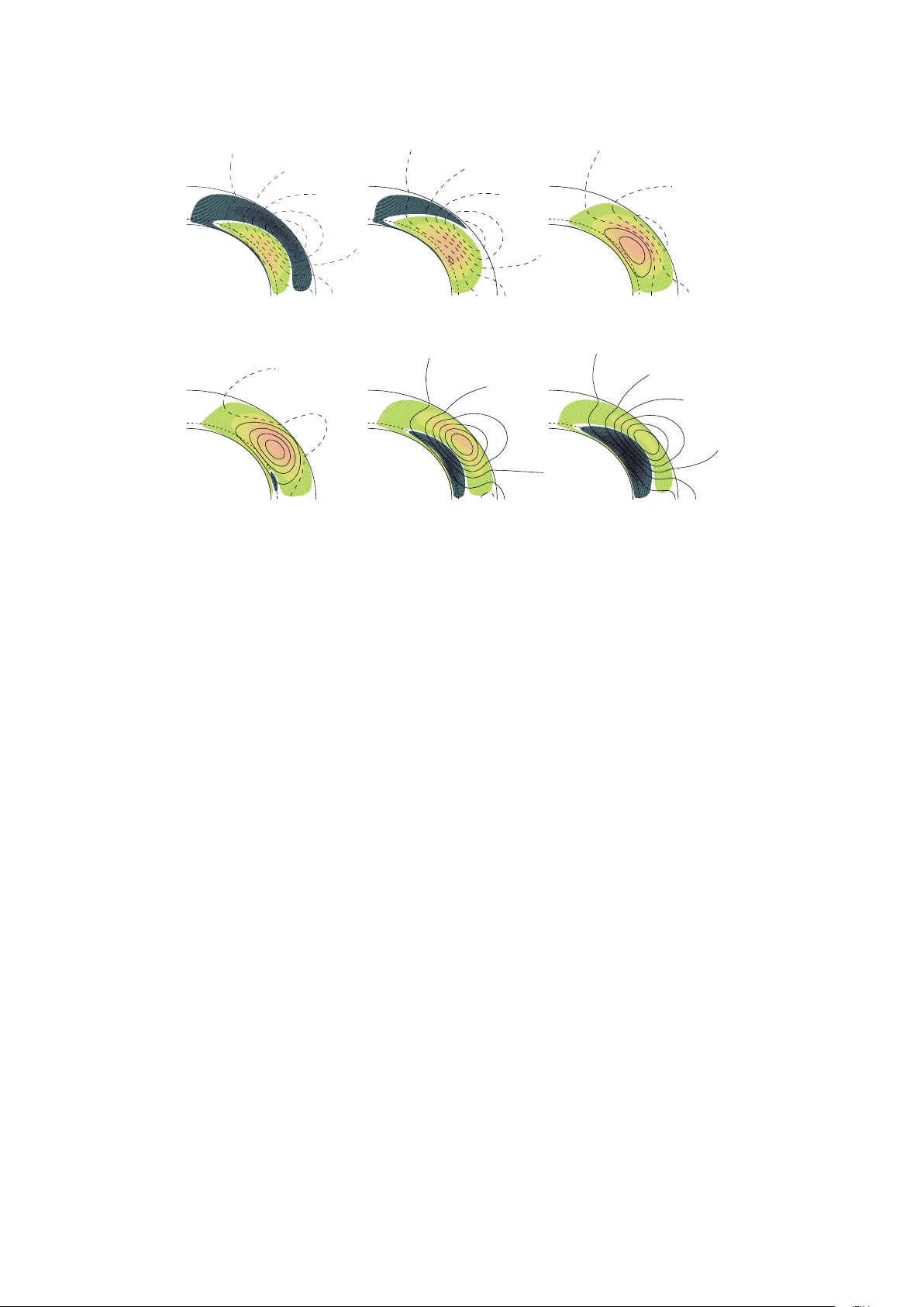
Benc hmarking the solar dynamo with Maxima ∗ V alery Pipin (Institute Solar-T errestrial Ph ysics, Irkutsk) No vem b er 16, 2021 Recen tly , Jouv e et al [2] published the pap er that presen ts the n umerical b enc hmark for the solar dynamo mo dels. Here, I would lik e to sho w a wa y how to get it with help of computer algebra system Maxima. This wa y was used in [4] to test some new ideas in the large-scale stellar dynamos. What y ou need are the latest version of Maxima-5.16.3 (preferable compiled against the fastest lisps like sb cl or cmucl-sse2) and some knowledge of the global (sp ectral) metho ds to solve the PDE eigen v alue problem. F or the quite comprehensive in tro duction to these metho ds please lo ok at the b o ok by John Boyd [1]. The basic steps to solve the problem are: 1. the mathematical form ulation (equation+boundary conditions) 2. choice the basis function and pro ject equations to the basis 3. find matrices (apply some in tegration pro cedure in case of Galerkin metho d) 4. apply linear algebra The whole consideration is divided for tw o cases. As the first case w e explore the largest free deca y mo des in the sphere whic h is submerged in v acuum. In this problem the all dynamo effects are neglected. As the second case I test the α Ω dynamo in the solar conv ection zone with the tachocline included. Lets consider the spherical geometry . The ev olution of the axisymmetric large-scale mag- netic field (LSMF), h B i = e φ B + curl  A e φ r sin θ  , (where r is radius, θ - co-latitude, e φ - the unit azim uthal v ector) in the turbulen t media sub jected to the differential rotation in the spherical shell can b e describ ed with equations: ∂ B ∂ t = 1 r ∂ (Ω , A ) ∂ ( r , θ ) + 1 r ∂  r E θ  ∂ r − ∂ E r ∂ θ ! , (1) ∂ A ∂ t = r sin θ E φ , (2) In equations ab o v e, the turbulent contribution is expressed through the comp onents of the mean electromotive force (MEMF) E = h u 0 × b 0 i , where u 0 , b 0 are the small-scale fluctuated v elo cit y and magnetic field resp ectively , Ω = Ω ( r , θ ) - the given angular v elo city distribution. F or the sake of simplicity we restrict consideration to the case of α Ω dynamo with isotropic turbulen t diffusion. Hence, w e ha v e E r = − η T r sin θ ∂ sin θ B ∂ θ (3) E θ = η T r ∂ r B ∂ r (4) r sin θ E φ = η T  ∂ 2 A ∂ r 2 + sin θ r 2 ∂ ∂ θ 1 sin θ ∂ A ∂ θ  + ˆ α ( r , θ ) η T GB r sin 2 θ (5) ∗ The text w ere pro cessed with Emaxima (h ttp://Maxima.sf.net) 1 where η T - turbulent diffusion, ˆ α ( r , θ ) - dimensionless function to mo del the α effect, G = ∇ log ρ - stratification parameter. W e adopt the model parameters given in [2]. The b oundary conditions are ∂ r B ∂ r = 0 , A = 0 - at the bottom and v acuum conditions - at the top of con vec- tion zone. F or the computation all the equations are written in dimensionless form with new radial co ordinate x = r/R  . Moreo v er, to pro ject equations on the basis function we use the co ordinate transformation to the in terv al where basis is orthogonal. As the first step we consider the solutions for the largest free-decay mo des. This intends to test the accuracy of the b oundary conditions implementation pro cedure and the sp eed of con vergence. W e neglect all the dynamo effects in (1, 2) and return to equations: ∂ B ∂ t = 1 x ∂ 2 ( xB ) ∂ x 2 + 1 x 2 ∂ ∂ θ 1 sin θ ∂ (sin θ B ) ∂ θ , (6) ∂ A ∂ t = ∂ 2 A ∂ x 2 + sin θ x 2 ∂ ∂ θ 1 sin θ ∂ A ∂ θ , (7) where for the sake of simplicity we hav e assumed that magnetic diffusivity is constan t ov er the depths and equations are written in dimensionless form. Lets consider the integration domain on the radial co ordinate to be x ∈ [0 , 1] and for latitude - from pole to pole. Ha ving the regular conditions at the origin and v acuum b oundary conditions at the top, w e can get the analytical solutions of (6, 7). They can b e expressed via the spherical Bessel functions. F or the sak e of simplicity we restrict ourselv es to solutions for the largest mo des. W e decomp ose the eigenmo des as follows B ( x, θ , t ) = e λt X n X m ˆ b nm S ( B ) n ( x ) P 1 m (cos ( θ )) , (8) A ( x, θ , t ) = e λt X n X m ˆ a nm sin ( θ ) S ( A ) nm ( x ) P 1 m (cos ( θ )) , (9) where P 1 m are the asso ciated Legendre p olynomials and other functions w ere found via basis recom bination of the Legendre p olynomials, namely , S ( B ) n ( x ) = x ( P 2 n +1 ( x ) − P 1 ( x )) , (10) S ( A ) nm ( x ) = x  P 2 n +1 ( x ) − P 1 ( x ) ((2 n + 1) (2 n + 2) + 2 ( m + 1)) (2 m + 4)  , (11) Her e, e ach element of b asis satisfies the b oundary c onditions individual ly . F or the largest deca y mo des w e ha ve S ( B ) 1 ( x ) ∝ j 1 ( αx ), λ = − α 2 ( α ≈ 4 . 4934) and S ( A ) 1 ( x ) ∝ j 1 ( π x ), λ = − π 2 . Similar to [3], the eigen vectors are scaled as S ( B ) 1 ( . 5) = 1 and S ( A ) 1 (1) = 1. The errors are measured as E ( λ ) = | λ true − λ num | and E ( B ) = R 1 0 | B true − B num | 2 dx . The results of b enc hmark are given in the T able 1. Next b enchmark is related to one giv en in the pap er [2]. The detail of the mo del can b e found in that pap er. W e consider the results for test B, whic h is for α Ω dynamo with external v acuum b oundary conditions and jump othe magnetic diffusivit y below the b otom of con v ection zone. F or the magnetic fields w e ha ve used the following set of the mo des: S ( B ) n ( x ) =  P n − 1 ( x ) − 13 (2 n + 1) P n ( x ) 13 n 2 + 26 n + 6 − (13 n 2 − 7) P n +1 ( x ) 13 n 2 + 26 n + 6  , (12) S ( A ) nm ( x ) = x  P n ( x ) + (2 n + 3) P n +1 ( x ) n 2 + 4 n + 2 m/f + 4 − ( n 2 + 4 n + 2 m/f + 1) P n +2 ( x ) n 2 + 4 n + 2 m/f + 4  , (13) 2 N E ( λ ) , B E (B) 3 3.83e-5 6.849e-4 4 9.984e-8 4.365e-9 5 1.207e-10 2.497e-12 6 8.707e-14 9.068e-16 7 1.77e-14 4.80e-19 8 5.32e-15 6.263e-23 E ( λ ) , A E (A) 1.08e-7 3.98e-9 5.651e-11 1.255e-12 9.68e-14 2.142e-16 7.72e-14 2.136e-20 1.38e-14 1.325e-24 1.90e-14 4.427e-29 T able 1: Con vergence of the decay mo des to the larges mo de of analytic solution of (6,7). N is the n um b er of mo des in radial basis. Resolution C crit α ω 8x8 .443 180.5 10x10 .4175 175.1 12x12 .4095 172.2 13x13 .411 172.4 14x14 .4122 172.7 16x16 .4125 172.9 T able 2: Mo del B of [2]. Resolution N × M means that N mo des is used in decomp osition on radius and M - on latitude. where factor f = 2 1 − x i app ears due the co ordinate transformation [ x i , 1] → [ − 1 , 1] and x i = 0 . 65 is b ottom of in tegration domain. The results are shown at the table 2 and Figure 1. Note, that our results are quite close to those in [2]. The small difference can be attributed to the difference in the metho d of solution of the problem. The largest deca y mo de of the diffusion op erator Here, I giv e some details of the abov e computation within Maxima. The strongest side of the computer algebra system is that most of the computational w ork is done exactly . F or example, all the deriv ativ es in (6, 7) are computed directly by substitution of (8, 9) to (6, 7). The integration ov er space domain has to b e done to pro ceed with the Galerkin metho d. This is carried out with help of the Gauss-Legendre pro cedure. The pro cedure is based on the so-called ”collo cation p oints and weigh ts” metho d. The collo cation p oints are the set of zeros of the Legendre p olynomial of the order > N where N is the num b er of the greatest mo de among n = 1 , . . . N in (8, 9). The collo cation p oin ts and w eigh ts can b e found via subprogram ”pseudp.mac”. It is giv en in App endix. The maxima session is started with the general definitions: kill(all)$ batchload("pseudp.mac")$ (xb:0.,xe:1.)$ bftorat:true$ float2bf:true$ ratprint:false$ fpprec:64$ ratepsilon:1.e-32$ 3 t=0.115 t=0.118 t=0.122 t=0.125 t=0.130 t=0.133 Figure 1: Mo del B of [2]. Snapshots of evolution of torioidal magnetic fileds (shado wed density plot) and p oloidal fields (sho wn with streamlines) o ver the half of cycle. chn(x):=x$ realGr(L1,L2):=(if realpart(L1) >= realpart(L2) then true else false)$ Here, w e find the collo cation points and w eights on radius, (np:5,Nch:4*np,xchwh:gaulegP(-1,1,Nch,1), xch:xchwh[1],wh:xchwh[2])$ and on latitude, (NT:6,NTT:6*NT,mut_w:gaulegP(-1,1,NTT,1),mut:mut_w[1],w:mut_w[2])$ Next, we define the indices for the basis functions and the parities for the toroidal and p oloidal eigenmo des, Nch:length(xch)$ NTT:length(mut)$ for m:1 thru NT do( for n:1 thru np do( ki:np*(m-1)+n,ni[ki]:n,mi[ki]:m))$ ni:makelist(ni[i],i,1,NT*np)$ mi:makelist(mi[i],i,1,NT*np)$ NN:NT*np$ parity_b:0$ parity_a:0$ 4 Note, that only a half of [ − 1 , 1] in terv als is used in computations. This leads to the computa- tional econom y and to increase the sp ectral resolution of the code. The follo wing are the part of the co de which defines the basis functions on radius ( S ( B ) n → chtb n , S ( A ) nm → chta nm ) and latitude, kill(chtb1,chtb)$ chtb[n](x):=x*(legendre_p(1,x)-legendre_p(2*n+1,x))$ makelist(taylor(chtb[i](x),x,0,1),i,1,np)$ plot2d(makelist(chtb[i](x),i,1,np),[x,-1,1])$ kill(chta00)$ chta00(n,l,x):=x*(legendre_p(2*n+1,x) -((2*n+1)*(2*n+2)+2*l+2)*legendre_p(1,x)/(2*l+4))$ chta[n,l](x):=chta00(n,2*l-1,x), kill(Pl10,Pla,Plb)$ Pl10(n,x):=expand((sqrt((2*n+1)/(2*n*(n+1)))*assoc_legendre_p(n,1,x)))$ Pla[n](x):=block(if parity_a=0 then bfloat(Pl10(2*n-1,x)) else bfloat(Pl10(2*n,x)) ) $ Plb[n](x):=block(if parity_b=0 then bfloat(Pl10(2*n-1,x)) else bfloat(Pl10(2*n,x)) ) $ As you see, w e use o dd or even asso ciated Legendre p olynomial in resp ectiv e of the parity c hoice. T o accelerate the in tegration pro cedure w e calculate the matrices of basis functions o ver the sets of collo cation p oin ts, remarray(PLB,PLA)$ kill(PLB1,PLA1)$ PLB[n,i]:=bfloat(Plb[n](mut[i]))$ PLA[n,i]:=bfloat(Pla[n](mut[i]))$ PLA1[n,i]:=bfloat(Pla[n](mut[i])*w[i])$ PLB1[n,i]:=bfloat(Plb[n](mut[i])*w[i])$ CHTB[n,j]:=bfloat(chtb[n](xch[j]))$ CHTA[n,m,j]:=bfloat(chta[n,m](xch[j]))$ makelist(makelist(makelist(CHTA[n,m,j],n,1,np),m,1,NT),j,1,Nch)$ CHTB1[n,j]:=bfloat(chtb[n](xch[j])*wh[j])$ CHTA1[n,m,j]:=bfloat(chta[n,m](xch[j])*wh[j])$ makelist(makelist(makelist(CHTA1[n,m,j],n,1,np),m,1,NT),j,1,Nch)$ genmatrix(PLB,NT,NTT)$ genmatrix(PLA,NT,NTT)$ genmatrix(PLA1,NT,NTT)$ genmatrix(PLB1,NT,NTT)$ genmatrix(PLB2,NT,NTT)$ genmatrix(CHTB,np,Nch)$ genmatrix(CHTB1,np,Nch)$ No w we can to pro ceed to solution of the problem (6, 7). They can b e treated separately . Firstly w e define the left parts of (6,7), kill(AA,BB)$ AA[ki,kj]:=bfloat(sum(CHTA1[ni[ki],mi[ki],j]*CHTA[ni[kj],mi[kj],j]* sum(PLA1[mi[ki],i]*PLA[mi[kj],i],i,1,NTT),j,1,Nch))$ BB[ki,kj]:=bfloat(sum(CHTB1[ni[ki],j]*CHTB[ni[kj],j] 5 *sum(PLB1[mi[ki],i]*PLB[mi[kj],i],i,1,NTT),j,1,Nch))$ BB:genmatrix(BB,NN,NN)$ AA:genmatrix(AA,NN,NN)$ Note, the integration is just a pro duct of sums o ver collo cation p oin ts. Now lets compute the righ t part of (6). The computations are straigh tforward. The radial part is, kill(CHTB_d2)$ CHTB_d2[n,j]:=bfloat(subst([x=xch[j]], expand((diff(diff(chtb[n](x),x),x) ))))$ genmatrix(CHTB_d2,np,Nch)$ kill(et_d)$ et_d[ki,kj]:=bfloat(sum(CHTB_d2[ni[kj],j]*CHTB1[ni[ki],j],j,1,Nch) *sum(PLB[mi[kj],i]*PLB1[mi[ki],i],i,1,NTT))$ et_d:genmatrix(et_d,NN,NN)$ The latitudinal part is computed as follo ws kill(PLB_d2,PLB_d2m,PLB_d1,PLB_d)$ PLB_d2m[n,i]:=bfloat(subst([mu=mut[i]],expand((sqrt(1-mu^2) *diff(diff(sqrt(1-mu^2)*Plb[n](mu),mu),mu)))))$ genmatrix(PLB_d2m,NT,NTT)$ kill(er_d)$ er_d[ki,kj]:=bfloat(sum(CHTB1[ni[ki],j]*CHTB[ni[kj],j]/chn(xch[j])^2,j,1,Nch) *sum(PLB1[mi[ki],i]*PLB_d2m[mi[kj],i],i,1,NTT))$ er_d:genmatrix(er_d,NN,NN)$ In vert the left part of and solve the eigen v alue problem with help of lapack BMI:invert_by_lu(BB)$ realGr0(L1):=(if realpart(L1) >=0 then true else false)$ load(lapack)$ MT:BMI.(er_d+et_d)$ lamb:(dgeev(MT,true))$ ... ;; Loading #P"/usr/share/maxima/5.16.3/share/lapack/lapack/binary-cmucl/dtrevc.sse2f". No w, lets sort the eigen v alues, lmb:sort(flatten((col(lamb,1))[1]),realGr); [- 20.19072855751148, - 48.83125052872499, - 59.68036461428608, - 87.54250816953108, - 108.8085726200047, - 119.8731393320569, - 135.9006458324267, - 169.2937978826357, - 193.7765731289586, - 203.8596788530381, - 238.1199364033153, - 241.2729384729356, - 260.8709651925637, - 277.930972796181, - 320.6253098224506, 6 - 328.0254017082749, - 373.0041226108443, - 410.8018157235754, - 505.412713312208, - 577.4557504236772, - 665.4381736491396, - 809.3382250971157, - 851.3024977594987, - 882.9750962899574, - 932.6139588501989, - 970.2769707279747, - 1049.716092377411, - 1259.650734653339, - 1830.07144488619, - 2585.672953057317] The relev ant spherical Bessel functions of the problem are jn(n,x):=spherical_bessel_j(n,x)$ jnR(n,x):=x*spherical_bessel_j(n,x)$ Next w e compute the first root of j n ( x ) and compare it with the first eigenv alue, a1:find_root(jn(1,x),x,4,5)$ sqrt(abs(first(lmb)))-a1; 1.207158817351228e-10 Similarly , w e solve (7). At the first, w e in vert the left part of it AMI:invert_by_lu(AA)$ Then calculate the righ t part and apply lapac k solv er, kill(CHTA_d2,PLA_d2)$ CHTA_d2[n,m,j]:=subst([x=xch[j]],(diff(diff(chta[n,m](x),x),x)))$ makelist(makelist(makelist(CHTA_d2[n,m,j],n,1,np),m,1,NT),j,1,Nch)$ PLA_d2[n,i]:=bfloat(subst([mu=mut[i]],(sqrt(1-mu^2) *diff(diff(sqrt(1-mu^2)*Pla[n](mu),mu),mu))))$ genmatrix(PLA_d2,NT,NTT)$ kill(ef_d)$ ef_d[ki,kj]:=bfloat(sum(CHTA_d2[ni[kj],mi[kj],j] *CHTA1[ni[ki],mi[ki],j],j,1,Nch)* sum(PLA1[mi[ki],i]*PLA[mi[kj],i],i,1,NTT) +sum(CHTA[ni[kj],mi[kj],j]*CHTA1[ni[ki],mi[ki],j] /chn(xch[j])^2,j,1,Nch)* sum(PLA1[mi[ki],i]*PLA_d2[mi[kj],i],i,1,NTT))$ ef_d:genmatrix(ef_d,NN,NN)$ MT:(AMI.ef_d)$ lamb:(dgeev(MT,true))$ Then, w e sort the eigen v alues and compare the largest eigen mo de with the first zero of J 1 / 2 ( x ), lmb1:sort(flatten((col(lamb,1))[1]),realGr)$ float(sqrt(abs(first(lmb1)))-%pi); - 9.681144774731365e-14 T o compare the eigenfunctions w e ha ve to apply the scaling S ( B ) 1 ( . 5) = 1 and S ( A ) 1 (1) = 1. The solution of dynamo problem is obtained in essentially the same wa y . I will put the co de for it somewhere in the public place. 7 References [1] J. P . Bo yd. Chebyshev and F ourie Sp e ctr al Metho ds . Dov er: NY, 2001. [2] L. Jouve, A.S. Brun, R. Arlt, A. Brandenburg, M. Dikpati, A. Bonanno, P .J. K¨ ap yl¨ a, D. Moss, M. Remp el, P . Gilman, M.J. Korpi, and A.G. Koso vic hev. A solar mean field dynamo bechmark. Astr on and Astr ophys. , 483:950–960, 2008. [3] P .W. Livermore and A. Jackson. A comparison of numerical schemes to solve the magnetic induction eigen v alue problem in a spherical geometry . Ge ophys. Astr ophys. Fluid Dyn. , 99:467–480, 2005. [4] V.V. Pipin and N. Seehafer. Stellar dynamos with Ω × J effect Astr on and Astr ophys. , in prin t, 2008. App endix The subroutine to find the collo cation p oints and w eghts for the p olynomial order of n in in terv al [ x 1 , x 2]. The Newton metho d is applied, load(orthopoly)$ orthopoly_returns_intervals:false$ fpprec:32$ float2bf:true$ ratprint:false$ load("linearalgebra")$ gaulegP(x1,x2,n):= block([xm,wm,A0,i,mm,pp,xm,xl,z,z1,numer,eps], kill(xt,w), eps:1.e-16,fpprec:32, (if oddp(n) then mm:(n+1)/2 else mm:n/2), xm:0.5*(x2+x1), xl:0.5*(x2-x1), for i: 1 while i <= mm do ( z:bfloat(cos(%pi*(i-0.25)/(n+0.5))), do (pp:bfloat(n*(z*legendre_p(n,z)-legendre_p(n-1,z))/(z*z-1.0)), z1:z,z:bfloat(z1-legendre_p(n,z)/pp), if abs(z-z1) < eps then return(z1)), xt[i]:xm-xl*z1, xt[n+1-i]:xm+xl*z1), A:bfloat(genmatrix(lambda([i,j],legendre_p(i-1,xt[j])),n,n)), RH:bfloat(transpose(matrix( makelist((if i=1 then defint(legendre_p(0,x),x,-1,1) else 0),i,1,n)))), w: bfloat(invert_by_lu(A) . RH), return([makelist(xt[i],i,1,n),flatten(makelist(w[i],i,1,n))]))$ 8