High-speed kinks in a generalized discrete $phi^4$ model

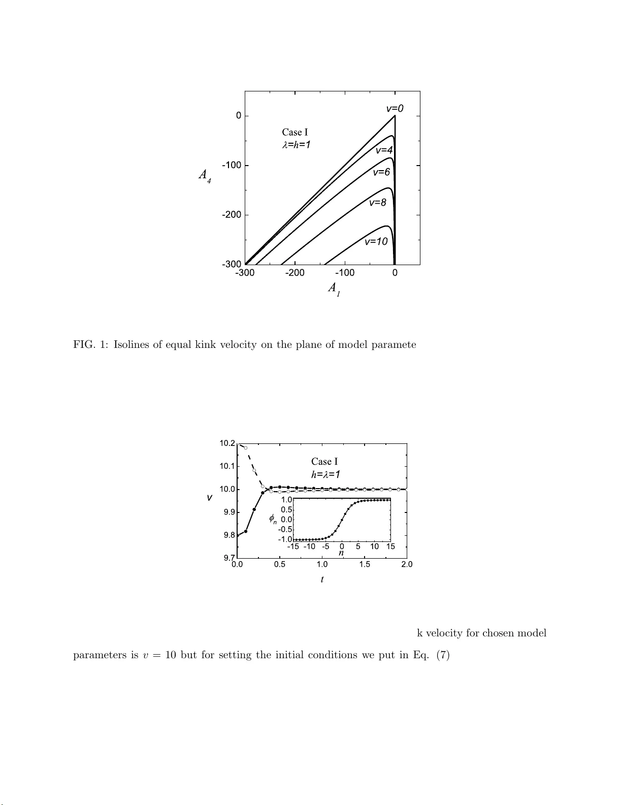
APS/123-QED High-sp eed kinks in a g eneralized discrete φ 4 mo del Sergey V. Dmitriev 1 , Avinash K ha re 2 , P ana y otis G. Kevrekidis 3 , Av adh Saxena 4 and Ljup´ co Hadˇ zievsk i 5 1 Institute for Metals Sup erplasticity Pr oblems RAS, 39 Khalturina, Ufa 450001, R ussia 2 Institute of Physics, Bhub aneswar, Orissa 75 1005, In d ia 3 Dep artment o f Mathematics an d Statistics, University of Massachusetts, A mherst, MA 0100 3-4515, USA 4 Center fo r Nonline ar Studies and T he or etic al Division, L os A la mos National L ab or atory, L os Alamos, New Mexic o 87545, USA 5 Vinc a I nstit ute of Nucle ar Sci e n c e, PO Box 522,11001 B elgr ade, Serbia (Dated: August 14, 2021) Abstract W e co nsider a generaliz ed discrete φ 4 mo del and d emo nstrate that it can supp ort exact moving kink solutions in t he form o f tanh with a n arbitrarily large v elo ci t y . T h e constructed exact mo ving solutions are dep enden t o n the sp ecific v alue of the propagation ve lo city . W e demonstrate that in this class of mo dels, giv en a sp ecific ve lo c it y , th e p roblem of fin d ing the exact moving solution is in tegrable. Namely , this pr o blem originally expressed as a three-p oin t map can b e r e duced to a tw o-p oin t map, from which the exact m oving solutions can b e d eriv ed iterativ ely . It w as also found that these high-sp eed kinks can b e stable and robust against p erturb at ions introd uced in the initial conditions. P ACS num b ers: 05.45.-a , 05.45.Yv, 63.20.-e 1 I. INTR ODUCTION Solitary wa v es pla y imp ortant role in a great v ariet y of applications b ec ause they are robust against perturbations and they can transp ort v arious phy sical quantities suc h a s mass, energy , momen tum, electrical c harge, and also info rmation [1, 2]. Many p opular con t inuum nonlinear equations supp ort tra v eling solutions, but for their discrete analogs the existence of trav eling solutions w as no t systematically studied un t il recen tly . Previously , only a few in tegrable lattices were kno wn to supp ort mov ing solitons, e.g., the T o da lattice [3] and the Ablowitz-Ladik lattice [4], the former b eing the discrete v ersion of the K d V equation and the la tter of the nonlinear Sc hr¨ odinger (NLS) equation. While integrable lattices of other k ey con t inuum models are also av ailable [5, 6], these integrable situatio ns are still rather exceptional and typic ally not directly relev an t to exp e rimen tal settings. On the other hand, recen tly sev eral wide classes of discrete mo dels supp orting translatio n ally in v ariant (TI) static or stationary solutions ha v e been discov ered and in v estigated for the discrete Klein-Gordon equation [7, 8, 9 , 10, 11, 12, 13, 1 4 , 15, 1 6, 17 , 18 , 19] and the discrete NLS equation [20, 21, 22, 2 3 , 24, 25]. Static solitary w a ve s in suc h lattices p ossess the translational Goldstone mo de [10, 18 , 19, 20, 21, 22], which means that the solitary w av es mo ving with vanishing v elo cit y can b e regarded as the exact solutions to these discrete equations (althoug h there are issues for finite but small v elo cities as explained e.g., in [26, 27]). Mo ving solutions pr o pagating along a lattice at finite v elo cit y ha ve also b een found analytically in [21, 22] and with the help of sp e cially tuned n umerical approache s in [2 4 , 26, 27, 28, 29, 30 , 31, 32]. T ra velin g bright solitons in the NLS lattice mo del with saturable nonlinearit y are also v ery interesting [27, 33, 34]. F o r this mo del the existence of soliton frequencies with v anishing Peie rls-Nabarro energy barrier w a s demonstrated. It w as sho wn that fo r the sp ecifi c f re quencies the static version of the mo del equation coincides with that of the integrable Ablowitz -Ladik equation [3 4]. This implies in the mapping analysis a p ossibilit y to reduce the three-p oin t map to a t wo-p oin t map. Ho wev er, the studied mo del equation is not integrable and while t he solitary w av es mo ving with small v elo cit y w ere nu merically obtained for the sp e cific frequencies, the question ab out the existence of solitary w av es mov ing with finite v elo cities remains op en. Existence of la ttice s supp orting the static TI solutions and t h e exact solutions mo ving with finite v elo cit y p oses a natural question, ab out whether there is a relation b et w een them. 2 In the presen t study w e answ er this question in the p ositiv e, creating a link b et w een these t wo classes of solutions b elo w. On the other hand, as regards the solitar y wa v e motion, another in teresting question is the existence of upp er b ound for the propagatio n v elo cit y . In view of Loren tz in v ariance, clearly the solitary w a ves in contin uum nonlinear equations of t he Klein-Gordon type hav e limitations on their pro pagation v elo cit y . One of the questions that w e examine b elo w is whether a similar restriction exists in the corresp onding discrete mo dels. Since the L o re n tz in v ariance is no longer a symmetry of the discre te nonlinear systems, strictly sp eakin g there need not be a ny restriction on the propaga tion v elo cit y . Ho w ev er, naiv ely one w ould exp ect that ty pically the propagation velocity in the discrete nonlinear system s w ould b e similar to the ones supp orted by their con tinuous counterparts and not dev elop sup e rsonic v alues. Recen tly , three o f us [22] confirmed t h is naiv e expectation in a generalized discrete NLS equation. A natura l question, how ev er, is whether this alwa ys holds true. Althoug h in some case examples, this has already b een a dd ressed [26 ], here w e address this question (and its negativ e answ er) more systematically in the framew o r k o f the recen tly studied discrete φ 4 mo del [19]: d 2 φ n dt 2 = 1 h 2 ( φ n +1 + φ n − 1 − 2 φ n ) + λφ n − A 1 φ 3 n − A 2 2 φ 2 n ( φ n +1 + φ n − 1 ) − A 3 2 φ n ( φ 2 n +1 + φ 2 n − 1 ) − A 4 φ n φ n +1 φ n − 1 − A 5 2 φ n +1 φ n − 1 ( φ n +1 + φ n − 1 ) − A 6 2 ( φ 3 n +1 + φ 3 n − 1 ) , (1) with the mo del parameters satisfying the normalization constraint 6 X k =1 A k = λ . (2) In Eq. (1) , φ n ( t ) is the unkno wn function defined on the lattice x n = hn with the lattice spacing h > 0. Without loss of generality it is sufficien t to consider the cases λ = 1 and λ = − 1. Our results will b e displa ye d a s follows. Analytical results are collected in Sec. I I. Examples of the exact mov ing solutions to Eq. (1) ar e giv en in Sec. I I A to Sec. II C. Then, in Sec. I I D, w e deriv e a con tinuum analog of Eq. (1) and find its kink solution. In Sec. I I E sp ectrum o f t he v acuum solution of Eq. ( 1 ) is obtained. The relatio n b et w een 3 the exact mo ving solutions and in tegrable maps is established in Sec. I I F. Section I I I is dev oted to the num erical analysis o f stabilit y and robustness of mo ving kinks. W e presen t our conclusions in Sec. IV. I I. ANAL YTICAL RESUL TS Our appro a c h to deriving analytical solutions will b e, at least in the b eginning of this section somewhat similar in spirit to the inv erse metho d of [35]. That is, w e will p ostulate the desired solution and will identify the mo de l parameters for whic h this solution will b e a v alid one, as w e explain in more detail b elo w. A. Mo ving sn solution It is easy to sho w that an exact solutio n t o Eq. (1) is φ n = A sn[ β ( hn + hx 0 − v t ) , m ] , (3) pro vided the f ollo wing relations are satisfied: A 5 ns(2 hβ , m ) = − A 3 ns( hβ , m ) , A 1 A 2 = − 2 mβ 2 v 2 , A 6 = 0 , (4) 2 A 2 h 2 = 2 A 4 ns( hβ , m )ns(2 hβ , m ) + A 2 ns 2 ( hβ , m ) − A 3 cs( hβ , m )ds( hβ , m ) − A 5 [cs(2 hβ , m )ds(2 hβ , m ) − ns 2 (2 hβ , m )] , (5) 2 − λh 2 A 2 h 2 = A 4 ns 2 ( hβ , m ) + A 2 cs( hβ , m )ds( hβ , m ) − A 3 ns 2 ( hβ , m ) + (1 + m ) β 2 v 2 A 2 . (6) In Eq. (3), A is the amplitude, v is the propagat io n v elo cit y , β is a parameter relat ed to the (in v erse) width, x 0 is an arbitrary p osition shift, 0 ≤ m ≤ 1 is the Jacobi elliptic function (JEF) mo dulus. F urther, ns( x, m ) = 1 / s n( x, m ) , cs( x, m ) = cn( x, m ) / sn ( x, m ) and ds ( x, m ) = dn( x, m ) / sn( x, m ), where sn( x, m ), cn( x, m ), and dn( x, m ) denote standard JEFs. 4 Solution parameters x 0 and m can b e chos en arbitrarily . Equations (4) to (6) establish fiv e constraints f rom whic h one can find the three solution parameters A , v , a n d β , and t w o constrain ts on mo del parameters h , λ , and A i ( i = 1 , 2 , ..., 6 ). It is po s sible to construct some other moving JEF solutions, fo r example, mo ving cn a n d dn solutions (and hence hyperb olic pulse solutions of the sec h t yp e) but w e do not discuss these here. B. Exact moving kink solution In the limit m → 1, the ab o ve movin g sn solution reduces to the mo ving kink solution φ ( x, t ) = tanh [ β ( hn + hx 0 − v t )] , (7) and the relations (4) to (6) take the simpler form β 2 = − A 1 2 v 2 , 2 A 3 = − A 5 (1 + T ) , A 6 = 0 , (8) 2 T h 2 = A 4 (1 + T ) + A 2 + A 5 2 (1 + 2 T − T 2 ) , (9) (2 − h 2 λ ) T h 2 = A 4 + A 2 (1 − T ) + A 5 2 (1 + T ) − A 1 T , (10) where T = tanh 2 ( hβ ) . (11) One can see that the solution is defined only if A 1 ≤ 0. It is w orth p oin ting out that the static [22] and the moving JEF as w ell as hyperb olic soliton solutions exist in this mo del in the follo wing sev en cases: (i) only A 2 nonzero (ii) only A 4 nonzero (iii) A 3 , A 5 nonzero (iv) A 2 , A 4 nonzero (v) A 2 , A 3 , A 5 nonzero (vi) A 3 , A 4 , A 5 nonzero (vii) as discussed ab o v e A 2 , A 3 , A 4 , A 5 all nonzero. F urther, while in t he static case, solutions exist only if A 1 , A 6 = 0, in the moving case solutions exist o nly if A 6 = 0 , A 1 6 = 0. It may b e noted that these conclusions are v alid for sn , cn , dn as w ell a s t a nh , sec h solutions. Moreo ver, while in the static case, the kink solution exists only if λ > 0, the mo ving kink solution is p ossible ev en when λ < 0. In fa c t, it turns o ut that in cases (i), ( ii) and (iii) kink solution with a large velocity v is p ossible only if λ < 0. While Eqs. (8) to (10) give a general set of restrictions on the mo del parameters sup- p orting the exact mo ving kink, b elo w w e extract and analyze three par t icular cases where the r estrictions attain a v ery simple and transparent fo r m . 5 Case I. Only A 1 , A 2 , and A 4 are nonzero. These parameters are sub ject to the constrain t of Eq. (2) and one can take A 1 ≤ 0 a nd A 4 ≤ A 1 − λ + 2 /h 2 as free parameters. F rom equations (8) to (1 0) and ( 2 ) w e get β 2 = − A 1 2 v 2 , A 4 = 2 h 2 − λ − A 1 T , A 2 = λ − A 1 − A 4 . (12) W e note that the kink v elo cit y v can hav e an arbitrary v alue in case λ > 0. Indeed, for c hosen λ and h , one can take any v and then, using the express ions of Eq. (12), find subsequen tly the in v erse kink width β and the remaining mo del parameters A 4 and A 2 . As a sub case of case I, one can tak e only A 1 and A 2 nonzero. F rom Eq. (12) w e get β 2 = − A 1 2 v 2 , 2 T = h 2 λ + 2 v 2 h 2 β 2 , A 2 = λ − A 1 . (13) F r o m here it is clear that the kink solution with large v is only p ossible in this case if λ < 0. Similar argumen ts are a ls o v alid in cases (ii) and (iii) discussed ab o v e. Case I I. Another intere sting case is when ( A 2 , A 3 , A 5 nonzero): A 2 = λ − 2 h 2 − A 1 , A 3 = λ − 2 h 2 − A 1 + A 4 , A 5 = − λ + 4 h 2 + A 1 − 2 A 4 , A 6 = 0 , (14) with A 1 and A 4 b eing free para m eters. It is clear that the constrain t o f Eq. (2) is satisfied for a n y A 1 and A 4 . Conditions (8) to (10) reduce to β 2 = − A 1 2 v 2 , A 5 = A 1 − λ T . (15) Th us, w e hav e a t wo-parameter set of mo ving kinks. Kink solution exists f or A 1 < 0 a nd A 4 > 2 /h 2 . In this case to o the kink v elo cit y v can o btain an y v alue. As it w as found in [1 9], for A 1 = 4 γ 1 λ, A 2 = 6 γ 2 λ, A 3 = (1 − 4 γ 1 − 8 γ 2 ) λ, A 4 = A 5 = 0 , A 6 = 2 γ 2 λ , (16) with a r b itrary γ 1 and γ 2 , the mo del Eq. (1) has the Hamiltonian H = X n h ˙ φ 2 n 2 + ( φ n − φ n − 1 ) 2 2 h 2 + λ 4 − λ 2 φ 2 n + γ 1 φ 4 n + γ 2 φ n φ n − 1 ( φ 2 n + φ 2 n − 1 ) +  1 4 − γ 1 − 2 γ 2  φ 2 n φ 2 n − 1 i , (17) 6 and hence energy is conserv ed in this mo del. Simple analysis o f Eqs. (8) to (10) suggests that among the mo dels supp orting t he exact movin g kink solutions there are no Hamiltonian mo dels. C. Exact moving trigonometric solution and mo ving four-p eriodic solution Exact moving trigon ometric solution. The discrete mo del of Eq. (1) supp orts an exact mo ving solution of the form φ n = A sin[ hβ ( n + x 0 ) − v t ] , (18) ev en when A i , i = 1 , ..., 6 are all no nzero provided λh 2 − 2 + 2 cos( hβ ) + v 2 = A 2 h 2 sin 2 ( hβ )[ A 3 − A 4 + (3 A 6 − A 5 ) cos( hβ )] , (19) A 1 + A 4 + A 3 cos(2 hβ ) + ( A 2 + A 5 ) cos( hβ ) + A 6 cos( hβ )[4 cos 3 ( hβ ) − 3] = 0 . (20) F r o m here, one can w ork out sp ec ific relations in the case of v arious mo dels. F or example, consider the Hamiltonian mo del with t he parameters satisfying Eq. (16) . It is easy to chec k that the moving sin e solution exists in this mo del provided λh 2 − 2 + 2 cos( hβ ) + v 2 = A 2 λh 2 sin 2 ( hβ )[1 − 4 γ 1 − 8 γ 2 + 6 γ 2 cos( hβ )] , (21) 4 γ 1 + (1 − 4 γ 1 − 8 γ 2 ) cos(2 hβ ) + 8 γ 2 cos 3 ( hβ ) = 0 . (22) Exact moving four-site p erio di c solution. F or β h = π / 2 the ab o v e moving tr ig onometric solution reduces to the mo ving fo ur-perio dic solution of the form φ n = A sin h π 2 ( n + x 0 ) − v t i , (23) with A 1 + A 4 = A 3 , A 2 = λh 2 − 2 + v 2 A 1 h 2 . (24) 7 F o r the Hamiltonian mo del, Eq. (24) reduces to γ 1 + γ 2 = 1 8 , A 2 = λh 2 − 2 + v 2 4 γ 1 λh 2 . (25) Ev en in t he Hamiltonian case the trigonometric solutio n can hav e a n arbitrarily large v elo c- it y . D. Appro ximate moving kink solution The discrete mo del of Eq. (1) with finite h can supp ort the solutio ns v arying slowly with n (the same class o f solutions can b e studied near the con tinuum limit, using h as a small expansion para m eter). F or suc h solutions one can use the expansion φ ( h ) ≈ φ + hφ x + (1 / 2) h 2 φ xx and substitute in Eq. (1) φ n = φ (0), φ n ± 1 = φ ( ± h ) to obtain φ tt = φ xx + λφ − λφ 3 − 1 2 h 2 B φ 2 φ xx − h 2 D φφ 2 x , (26) where B = A 2 + 2 A 3 + 2 A 4 + 3 A 5 + 3 A 6 , D = A 3 − A 4 − A 5 + 3 A 6 , (27) and Eq. (2) w as used. F or B = D = 0 Eq. (26) reduces to the con tin uum φ 4 equation. This equation a ls o stems from Eq. (26) in the limit h → 0. Equation ( 2 6 ) supp orts the follo wing kink solution φ ( x, t ) = tanh [ β ( x + x 0 − v t )] , (28) pro vided the f ollo wing t wo conditions ar e satisfied β 2 = λ 2 (1 − v 2 ) + h 2 D , B + D = 0 . (29) This is the quasi-contin uum analog of the solution of Eq. (7 ). Let us analyze the case of λ = 1, whic h corresp onds to the double-w ell p oten tial. F or D = B = 0 or/and h = 0 w e ha ve the classical con t inuum φ 4 kink with the propag ation velocity limited as | v | < 1. On the o the r hand, for nonzero D = − B and nonzero h , there is no limitation on the kink propagation v elo cit y . In other w ords, fast kinks are p ossible in Eq. (26) only in the presence 8 of sev era l comp eting nonlinear terms. Note that in case B , D 6 = 0, Eq. (26) is no t Loren tz in v ariant. F o r wide kinks, i.e. when β ≪ h , one can use the kink solution of Eq. (26) to write do wn the appr oxima t e solution to the discrete mo del Eq. (1) of the form of Eq. (7), whose parameters are g iv en b y Eq. (2 9 ) . The correspo nding wide, fast kinks are p ossible in Eq. (1) o nly fo r finite h and only for D = − B 6 = 0. Substituting the Hamiltonian conditio ns of Eq. (16) into Eq. (27) we find B = 2 D while, according to Eq. (29), the appro ximate moving kink solution exists at B = − D , i.e., it exists only in non- Hamiltonian discrete mo dels. E. Sp ectrum of v acuum The discrete mo del of Eq. (1) supp orts the v acuum solutions φ n = ± 1. The spectrum of the small-amplitude w av es (phonons) of the f orm ε n ( t ) ∼ exp( ik n ± iω t ), propa gating in the v acuum, is ω 2 = 2 λ + 2  2 h 2 − B  sin 2  k 2  , (30) where k denotes w av en umber, ω is frequency and B is a s giv en by Eq. (27). Another v acuum solution, φ n = 0, supp orts the phonons with the disp ersion relation ω 2 = − λ + 4 h 2 sin 2  k 2  , (31) and this v acuum is stable for λ < 0. F. Relation t o TI mo dels Note that fo r v = 0 the exact moving solutions Eq. (3), Eq. (7 ), and Eq. (18) reduce to the static TI solutions, i.e., solutions whic h, due to the presence of arbitrary shift x 0 , can b e placed an ywhere with resp ect to the lattice. TI solutions o f Eq. (1) w ere discussed in detail in [19]. P a rticu larly , it w a s established that an y TI static solution can b e obtained iterativ ely from a t wo-p oin t nonlinear map. Let us demonstrate that the exact mo ving solutions (including JEF solutions) can also b e deriv ed from a map. Let us generalize the ansatz Eq. (3) and lo ok for moving solutions to Eq. (1 ) of the form φ n = AF ( ξ ) , ξ = β ( hn + hx 0 − v t ) , (32) 9 with constant a m plitude A , where F is suc h a function that d 2 φ n dt 2 = − β 2 v 2 ( α 0 φ n + α 1 φ 3 n ) , (33) with constan t co efficien ts α 0 , α 1 . If this is the case, the substitution of Eq. (32) into Eq. (1) will result in a static pro ble m essen tially identical to the static form of Eq. (1), namely , in the pro ble m 0 = 2 h 2 ( φ n − 1 − 2 φ n + φ n +1 ) + 2( λ + α 0 β 2 v 2 ) φ n − 2( A 1 − α 1 β 2 v 2 ) φ 3 n − A 2 φ 2 n ( φ n − 1 + φ n +1 ) − A 3 φ n ( φ 2 n − 1 + φ 2 n +1 ) − 2 A 4 φ n − 1 φ n φ n +1 − A 5 φ n − 1 φ n +1 ( φ n − 1 + φ n +1 ) − A 6 ( φ 3 n − 1 + φ 3 n +1 ) . (34) This effectiv e separatio n of the spatial and temp oral pa r t with each of them satisfying appropriate conditions is reminiscen t of the metho d of [36]. The Jacobi elliptic functions a nd some of their complexes do p ossess this prop ert y . F or example, Eq. (33) is v alid f or α 0 = 1 + m , α 1 = − 2 m A 2 , for F = sn ; α 0 = 1 − 2 m , α 1 = 2 m A 2 , for F = cn ; α 0 = m − 2 , α 1 = 2 A 2 , for F = dn; α 0 = 1 + m , α 1 = − 2 A 2 , for F = 1 sn ; α 0 = 1 − 2 m , α 1 = 2( m − 1) A 2 , for F = 1 cn ; α 0 = 2(2 m − 1) , α 1 = − 2 A 2 , for F = sndn cn . (35) In the limit m = 1 w e get from the first line of Eq. (35) α 0 = 2 , α 1 = − 2 , for F = tanh . (3 6) A solution mo ving along the c hain con tin uo us ly passes through all configurations betw een the o n- s ite and the inter-site ones. If one finds a static solution to Eq. (34) t ha t exists fo r an y lo cation with respect to the lattice, then one finds the corresp onding mo ving solutio n to Eq. (1). V arious static solutions to Eq. (34) that ha ve the desired prop ert y o f translational 10 in v ariance hav e b een recently constructed. Let us discuss the tw o simple cases sp ecified in Sec. I I B. Case I . F o r nonzero A 1 , A 2 , and A 4 = λ − A 1 − A 2 , Eq. (1) reduces to d 2 φ n dt 2 = 1 h 2 ( φ n − 1 − 2 φ n + φ n +1 ) + λφ n − A 1 φ 3 n − A 2 2 φ 2 n ( φ n +1 + φ n − 1 ) − A 4 φ n − 1 φ n φ n +1 , (37) while from Eq. (34) we get 1 h 2 ( φ n − 1 − 2 φ n + φ n +1 ) + ( λ + α 0 β 2 v 2 ) φ n − ( A 1 − α 1 β 2 v 2 ) φ 3 n − A 2 2 φ 2 n ( φ n +1 + φ n − 1 ) − A 4 φ n − 1 φ n φ n +1 = 0 . (38) Setting A 1 = α 1 β 2 v 2 , α 0 = − α 1 , (39) w e r educe Eq. (38) to the in tegrable static equation [17] 1 h 2 ( φ n − 1 − 2 φ n + φ n +1 ) + P φ n − A 2 2 φ 2 n ( φ n +1 + φ n − 1 ) − ( P − A 2 ) φ n − 1 φ n φ n +1 = 0 , (4 0) with P = λ − A 1 . (41) An y static TI solution to Eq. (40) generates the corresp onding mo v i n g solution to Eq. (3 7), pro vided that Eq. (33) is satisfied. All static solutions of Eq. ( 4 0) can b e found from its first integral [19 ], φ 2 n + φ 2 n +1 − Y φ 2 n φ 2 n +1 2 − P h 2 − 2 Z φ n φ n +1 − C Y 2 − P h 2 = 0 , Z = (2 − P h 2 ) 2 − C h 4 ( P − A 2 ) 2 2 (2 − P h 2 ) + C h 4 A 2 ( P − A 2 ) , Y = h 2 ( P − A 2 + A 2 Z ) , (42) where C is the in tegr a tion constant. The first integral can b e view ed as a nonlinear map from whic h a particular solution can b e f ound iterativ ely for an admissible initial v a lue φ 0 and for a chos en v a lue of C . 11 Th us, Eq. (42) is a general solution to Eq. (40 ), while to mak e it also a solution of Eq. (38) one needs to satisfy Eq. (39). This can b e achiev ed b y calculating d 2 φ n /dξ 2 from the map Eq. (42) a nd equalizing it to − α 0 φ n +1 − α 1 φ 3 n +1 according to Eq. (33). T o calculate d 2 φ n /dξ 2 w e consider a static solution cen tered at the lattice p oin t with the n um b er n so that φ n = 0. F r o m the map Eq. (42 ) one can find φ n +1 (0) = p C Y / (2 − P h 2 ). W e then consider the initial v alues φ n = − ε and φ n = ε and similarly , fro m the map Eq. (42), find the correspo nding v alues of φ n +1 ( − ε ) a nd φ n +1 ( ε ). F inally , w e calculate the second deriv a tiv e at the p oin t n + 1 as d 2 φ n /dξ 2 = lim ε 2 → 0 [ φ n +1 ( − ε ) − 2 φ n +1 (0) + φ n +1 ( ε )] /ε 2 = − α 0 φ n +1 − α 1 φ 3 n +1 , where the v alues of the co efficien ts are α 0 = C Y 2 − (2 − P h 2 ) 2 ( Z 2 − 1) (2 − P h 2 ) C Y , α 1 = − 2 C . (43) Let us summarize our findings. F rom Eq. (43) and the second expression of Eq. (39), taking in to accoun t Eq. (41), w e find the relation b et w een the integration constant C and mo del parameters A 1 , A 2 , λ , and h when a mov ing solution is p ossible : (1 − C ) P  2 − P h 2  2 × h h 4 ( C − 1) P 3 + C h 4 A 2  5 A 2 P − 4 P 2 − 2 A 2 2  +4  2 A 2 − 3 P − A 2 P h 2 + 2 P 2 h 2  i = 0 . (44) The solution profile is fo u nd for this C from Eq. (42) iteratively for an admissible initial v alue φ 0 , and the pro pagation v elo cit y v is fo und from the first expression of Eq. (39) and the second expression of Eq. (43). F ollow ing this wa y , any mov ing solution to Eq. (37) can b e constructed (p ossibly , except for some v ery sp ecial solutions that may arise from factorized equations [1 9 ]) . Note that in [17] we could express many but not all the solutions of Eq. (40) in terms of JEF. The approac h deve lop ed in this section allows one to obtain iterativ ely ev en those mo ving solutions whose corresp onding static problems w ere not solv ed in terms of JEF. The simplest case is C = 1 when Eq. (44) is satisfied and this case corr esp onds to the kink solution. F rom Eq. (43) w e find α 0 = 2 , α 1 = − 2 , (45) whic h coincides with Eq. (36). The map Eq. (42) in this case reduces t o ± s (2 /h 2 ) − A 4 λ − A 1 ( φ n − φ n +1 ) − φ n φ n +1 + 1 = 0 . (46) 12 One can chec k that Eq. (46 ) suppor t s the static solution φ n = tanh[ hβ ( n + x 0 )] with tanh 2 ( β h ) = λ − A 1 2 /h 2 − A 4 , (47) and this coincides with the second expression of Eq. (12 ). The static solution Eq. (47), that can also b e found iteratively from Eq. (4 6 ), giv es the profile of the moving kink that satisfies Eq. (37). The kink v elo cit y v is found from Eq. (39) and Eq. (45) and this a gree s with the first expression o f Eq. (12). Case I I. The mo del parameters are related b y Eq. (14) with A 1 and A 4 b eing free parameters. F o r A 1 = − 2 β 2 v 2 , Eq. (34) reduces to 2 h 2 ( φ n − 1 − 2 φ n + φ n +1 ) + 2 ( λ − A 1 ) φ n − A 2 φ 2 n ( φ n − 1 + φ n +1 ) − A 3 φ n  φ 2 n − 1 + φ 2 n +1  − 2 A 4 φ n − 1 φ n φ n +1 − A 5 φ n − 1 φ n +1 ( φ n − 1 + φ n +1 ) = 0 , (48) whic h is a particular form of the case (vii) static equation studied in [19 ]. The first in tegra l of the static mo del (vii) for the general case is not kno wn, but it is known for an y particular JEF solution [19]. Let us further simplify t he pro ble m considering only the kink solution of Eq. (48), for whic h one has tanh 2 ( hβ ) = A 1 − λ A 5 . (49) This relation coincides with the second expression of Eq. (15). F rom the kno wn static tanh solution one can deduce the following t w o-p oin t map that generates this solution for any initial v a lue | φ 0 | < 1: φ n +1 = φ n ± p ( A 1 − λ ) / A 5 1 ± φ n p ( A 1 − λ ) / A 5 , (50) where one can inte rc hange φ n and φ n +1 and tak e either the upp er or the low er sign. The static kink solutio n to Eq. (48) with β satisfying Eq. (49), that can also b e found iterativ ely from Eq. (50 ), giv es the profile of the moving kink that satisfies Eq. (1) with the parameters related b y Eq. (14). The kink v elo cit y v is found from Eq. (39) and Eq. (45). I I I. NUMERICS Let us analyze t he kink solutions for the cases I and I I describ ed in Sec. I I B. Only the case of λ = 1 will b e ana ly zed. 13 - 3 0 0 - 2 0 0 - 1 0 0 0 - 3 0 0 - 2 0 0 - 1 0 0 0 C a s e I = h = 1 v= 4 v= 6 v= 8 v= 1 0 v= 0 A 4 A 1 FIG. 1: Isolines of equal kink vel o c it y on the p la ne of mo del parameters A 1 , A 4 for the Case I at λ = h = 1, A 2 = λ − A 1 − A 4 , A 3 = A 5 = A 6 = 0. 0 . 0 0 . 5 1 . 0 1 . 5 2 . 0 9 . 7 9 . 8 9 . 9 1 0 . 0 1 0 . 1 1 0 . 2 - 1 5 - 1 0 - 5 0 5 1 0 1 5 - 1 . 0 - 0 . 5 0 . 0 0 . 5 1 . 0 n C a s e I h = = 1 v t n FIG. 2: Kink v elo cit y as a fu nctio n of time for the C a se I. The exact kink v elo cit y for c h o sen model parameters is v = 10 but for setting the initial conditions w e p ut in Eq. (7) v = 9 . 8 (dots) and v = 10 . 2 (op en circles). In b oth cases, regardless of the sign of p erturbation, the kink ve lo city rapidly approac hes the exact v alue. T he inset sho ws th e moving kin k profile. Mod el parameters: λ = h = 1, A 1 = − 20, A 4 ≈ − 222 . 1, A 2 = λ − A 1 − A 4 , A 3 = A 5 = A 6 = 0. 14 In our simulations we solve the set of equations of mot io n, Eq. (1), numeric ally with a sufficien tly small time step τ using the Stormer in tegration sc heme of order O ( τ 6 ). Initial conditions a re set b y utilizing Eq. (7) with v arious parameters. Anti-perio dic or fixed b oundary conditions ar e emplo y ed. A. Exact mo ving kinks in C ase I In this case, a s it was already men tio ned, the exact mo ving kink solution exists for the free mo del parameters satisfying A 1 ≤ 0 and A 4 ≤ A 1 − λ + 2 /h 2 (see Fig. 1 where for λ = h = 1 we show the isolines of equal kink v elo cit y o n the plane of mo del para me ters A 1 , A 4 ). On the line A 1 = 0, according to the first expression of Eq. (12), the kink v elo cit y v v anishes. On the line A 4 = A 1 − λ + 2 / h 2 the kink ve lo cit y also v anishes. This is so b ecaus e, as it can b e seen from the second expression of Eq. (12 ), on this line we hav e T = 1, i.e. β → ∞ a nd kink width v anishes. On the line A 4 = A 1 − λ + 2 /h 2 w e a lso hav e B = 2 /h 2 , whic h corresp onds to v anishing of the width of the phonon sp ectrum g iv en b y Eq. (30). The v acuum φ n = ± 1 is stable, i.e. the sp ectrum Eq. (30) do es not ha ve imaginary frequencies, if A 4 < A 1 + 2 /h 2 , i.e., it is stable in the whole region where the exact mo ving kink solution is defined. As it w as already men tioned, the kink propagation velocity is unlimited a nd fr om Fig. 1 one can see tha t | A 4 | increases fo r higher kink ve lo cities while A 1 can hav e a n y negativ e v alue. F or example, for v = 10 the mov ing kink exists for A 1 < 0 and A 4 < − 221 . 9. Let us now turn to the discussion of the stabilit y of moving kinks. Case of λ = h = 1 and v = 10 . Mo ving kink solutions are stable not in the whole range of parameters of their existence but for eac h studied v alue o f propagation v elo cit y w e w ere able to find a range of para m eters where the mo ving kink is stable in the sense that ev en a p erturb ed kink solution (with a reasonably large p erturbation amplitude) in course of time tends to t he exact solution (i.e., it is effectiv ely “attra c tiv e”). The ev olution of t he kink velocity in such self-regulated kink dynamics is sho wn in Fig. 2 for a v elo cit y a s large as v = 10 for A 1 = − 20 at λ = h = 1 . F o r this c hoice, w e ha ve f rom Eq. (12) β ≈ 0 . 316, A 4 ≈ − 222 . 1, A 2 ≈ 2 4 3 . 1. The moving kink profile is sho wn in the inset of Fig. 2. The p erturbation w as in t r o duced in to the initial conditions b y setting in the exact solution o f Eq. (7), a “wrong” propaga t ion v elo cit y , 15 smaller or hig her than the exact v alue v = 10. It can b e seen that in course of time the propagation velocity approac hes the exact v alue regardless of the sign of p erturbation. The increase of kink velocity launc hed with v = 9 . 8 ma y lo ok coun terin tuitiv e but one should k eep in mind that moving kinks are the solutions to a non-Hamiltonian ( o pen) system with the p ossibilit y to hav e energy exc hange with the surroundings with gain or loss, dep en ding on the tra jectories of particles (see, e.g., [10]). W e found that the absolutely stable, self-r egula t e d motion of kink, similar to that sho wn in Fig. 2, for v = 10 and λ = h = 1 tak es place within the range of − 164 < A 1 < − 1 . 1. The in ve rse kink width at the low er edge of the stability windo w is β ≈ 0 . 9 0 6, whic h corresp onds to a rather sharp kink, while for A 1 = − 1 . 1 (the upp er edge of the stabilit y windo w) one has β ≈ 0 . 0742 and the kink is m uch wider than the lattice spacing h . F or comparison, the kink sho wn in the inset o f Fig. 2 has β ≈ 0 . 3 1 6. F or A 1 < − 164 the mo ving kink solution b ecome s unstable and displacemen ts of particles b ehind the kink grow rapidly with time resulting in the stopping of nume rical run due to floating p oin t ov erflo w. F or − 1 . 1 < A 1 < 0 kink dynamics is as describ ed in Sec. 6 of [10 ] for the non-Hamiltonian case. In this region of parameter A 1 , after a transition p eriod, the kink starts to excite in the v acuum in its w a k e a wa v e with constant amplitude. In this regime, the kink attains a constan t ve lo cit y whose v alue is, generally sp eaking, different from that prescribed b y Eq. (1 2). Kink dynamics in the t w o unstable regimes describ ed ab o ve will b e illustrated below for the kinks mo ving with v < 1. Case of λ = h = 1 and v < 1 . Similar results w ere obtained fo r the kinks mo ving with small v elo cities ( v < 1). F or smaller v elo cities the range of A 1 with stable, self-regulated motion b ecomes narrow er. F or instance, a kink with v = 0 . 8 is stable (in the ab o v e men tio ne d sense) for − 2 . 4 < A 1 < − 0 . 10, while the one with v = 0 . 5 for − 0 . 19 < A 1 < − 0 . 06. In Fig. 3 w e sho w the time v ariation of the mo ving kink profile to demonstrate the instabilit y of the exact kink solution mo ving with v = 0 . 8 at A 1 = − 2 . 6. This solution is unstable and, due to the presence of rounding error p erturbation, the w av e b ehind the kink is excited. The amplitude of the w av e rapidly grows with time and it b ecomes noticeable in the scale of the figure a t t > 100. A t t ≈ 130 the n umerical r u n stops due to the floating p oin t ov erflow. Kink v elo cit y is nearly equal to v = 0 . 8 practically un til the collapse of the w av e b ehind it. 16 In Fig. 4 w e show the kink v elo cit y a s a function o f time t o illustrate the instabilit y o f the exact mo ving kink solution at v = 0 . 8 and A 1 = − 0 . 07. This solution is unstable and, due to the presence of r oundin g error p erturbation, at t ≈ 4 00 it starts to t r ans form in to an oscillating kink (with the p erio d T ≈ 5 . 01) moving with differen t velocity and exciting a constan t-a mp litude wa v e b ehind it. The transformation is essen tially complete b y t ≈ 50 00 and the kink v elo cit y b ecomes v ≈ 0 . 96. The inset shows the profiles of an oscillating mo ving kink in the tw o configura t io ns with t he most deviation from the av erage in time configuration. Case of λ = 1 , h = 0 . 1 , and v = 1 0 . Stable, self-regulated motion o f high-sp eed kinks w as a ls o observ ed for a s small lattice spacing as h = 0 . 1. This may app ear surprising at first sight b e cause for small h one w ould exp ect the discrete mo del to b e close to the contin uum φ 4 mo del where pro pa g ation with the velocity faster than v = 1 is imp ossible. But lo oking at Eq. (26), one can no tic e that the t wo last non-Lor e n tz-inv arian t terms hav e the co efficie n ts h 2 B and h 2 D , a nd they are not small ev en for small h if B and D are large. The high-sp eed kink in the considered case indeed exists for B ≈ − 19833 . 1 and D ≈ 2 0034 . 1. These v a lue s corresp ond to the follo wing pa rame ters considered in this n umerical run: A 1 = − 200 . 0, A 4 ≈ − 20034 . 1 , A 2 = λ − A 1 − A 4 ≈ 20235 . 1, A 3 = A 5 = A 6 = 0, β = 1. B. E xac t mo ving kinks in Case I I In the case I I, the mo del parameters a re related b y Eq. (14) and w e find B = − 2 A 4 + 6 /h 2 . As it w as already men tioned, the exact mo ving kink solution exists fo r A 1 < 0 and A 4 > 2 /h 2 . Isolines of equal kink velocity on the plane of the free mo del parameters A 1 , A 4 can b e seen in Fig. 5 for λ = h = 1. In t he Case I I, similarly to the Case I, on the borders of the existence of the kink solutio n the kink velocity v anishes. Moreo v er, on the b order A 4 = 2 /h 2 , b oth the width of the phonon sp ectrum given b y Eq. (30) and the kink width v a nis h, and this is also similar to what we saw in Case I. As was men tioned ab o ve , the exact mo ving kink solutio n in the Case I I can also hav e arbitrary v elo cit y . Kink dynamics in the Case I I w as observ ed to b e qualitativ ely similar to that of t he Case I. F or the kink with sp eed as large as v = 1 0 for λ = h = 1 w e found that the absolutely stable self-regulated motion is observ ed within the range of − 82 < A 1 < − 1 . 0. 17 - 1 0 1 - 1 0 1 - 1 0 1 - 4 0 - 3 0 - 2 0 - 1 0 0 1 0 2 0 - 1 0 1 t = 0 ( a ) n t = 1 0 0 ( b) n t = 1 1 0 ( c ) n t = 1 2 0 ( d) n n FIG. 3: Change of the mo ving kink p rofile d emons t rating the instabilit y of the exact solution for the follo wing set of mod e l parameters: λ = h = 1, A 1 = − 2 . 6, A 4 ≈ − 2 . 538, A 2 = λ − A 1 − A 4 ≈ 6 . 138, A 3 = A 5 = A 6 = 0. Exact kink p a rameters are v = 0 . 8, β ≈ 1 . 425. This solution is unstable and, d ue to the p resence of roundin g err o r p erturbation, the w av e b ehind the kink is excited. The amplitude of the wa v e rapidly gro wths with time and it b ecomes noticeable in the scale of the figure at t > 10 0. A t t ≈ 13 0 the numerical run stops due to the floating p o in t ov erflo w. The correspo nding inv erse kink width v aries in the range 0 . 640 < β < 0 . 0707. F or A 1 < − 82 the mo ving kink solution b ec omes unstable and displacemen ts of particles in the w a ke of the kink grow ra pidly with time resulting in the termination of nume rical run due t o floating p oin t o verflo w. F or − 1 . 0 < A 1 < 0, after a transition p erio d, the kink starts to excite in the v acuum b ehind itself a wa v e with constan t amplitude. In this regime, the kink propa gates with a constan t ve lo cit y whose v alue is, generally sp e aking, differen t from that prescrib ed b y Eq. (15). C. Exact moving four-p erio dic solution W e ha v e studied the dynamics of the exact moving four- s ite p erio dic solutio n Eq. (23) in the Hamiltonian mo del, i.e., with the parameters satisfying Eq. (2 5). Pe rio dic b oundary conditions w ere emplo y ed for a c hain of 40 particles. A small p erturbation w as introduced 18 0 1 0 0 0 2 0 0 0 3 0 0 0 4 0 0 0 5 0 0 0 0 . 8 0 0 . 8 4 0 . 8 8 0 . 9 2 0 . 9 6 - 1 5 - 1 0 - 5 0 5 1 0 1 5 - 1 . 0 - 0 . 5 0 . 0 0 . 5 1 . 0 C a s e I h = = 1 v t n n FIG. 4: Kink velocit y as a function of time demonstrating the instability of the exact moving kink solution for th e follo win g set of m odel p arameters: λ = h = 1, A 1 = − 0 . 07, A 4 ≈ − 18 . 28, A 2 = λ − A 1 − A 4 ≈ 19 . 35, A 3 = A 5 = A 6 = 0. Exact kink parameters are v = 0 . 8, β ≈ 0 . 234. This solution is u nstable and , du e to th e presence of roun ding error p erturbation, at t ≈ 400 it starts to transform to an oscillating mo ving kink (with the p erio d T ≈ 5 . 01). The transformation is essen tially complete by t ≈ 5000. Inset shows the pr o files of the oscillating moving kink in the t wo configurations with th e m o st deviation from the a v erage in time configuration. - 1 0 0 - 8 0 - 6 0 - 4 0 - 2 0 0 0 2 0 4 0 6 0 8 0 1 0 0 v= 2 C a s e I I = h = 1 v= 4 v= 6 v= 8 v= 1 0 v= 0 A 4 A 1 FIG. 5: Isolines of equal kink v elo cit y on the p la ne of mo del parameters A 1 , A 4 at λ = h = 1 for the case I I when mo del parameters satisfy Eq. (14). 19 in t he amplitude of particles at t = 0 and w e alw ays observ ed a growth of deviation of the p erturbed solution aw ay from the exact one. W e v aried the free mo del parameter γ 1 and the solutio n pa rame ter v in wide ranges at λ = h = 1 but could not find a stable regime. IV. CONCLUSIO NS F o r the discrete mo del of Eq. (1), in Sec. I I A w e obtained exact mo ving solutions in the form of the sn Jacobi elliptic function. Solutions in the fo rm of cn and dn Jacobi elliptic functions can also b e constructed as well as the solutions having the form of 1/sn, 1/cn, and sndn/cn in analogy with [17]. In Sec. I I B, from the sn solution, in the limit of m → 1, w e extracted the exact mo ving kink solution in t h e form of tanh, i.e., the corresp onding h yp erb olic function solution. Setting v = 0 in the exact mo ving solutions o btained in this w o rk one obtains the TI static solutions r ep orted in [19]. In this sense, the results rep orted here generalize o ur previous results. W e th us reve al the hidden connection b et w een the static TI solutions a nd the exact mo ving solutions. Suc h solutions can b e deriv ed from a t hr ee-p oin t map reducible to a t wo-po in t map (see Sec. I I F) i.e., f r o m an integrable map [3 7 ]. W e ha ve demonstrated t ha t the exact moving solutions to lattice and contin uo us equa- tions with comp eting nonlinear terms can ha ve any large propagation v elo cit y . Most of the hig h-speed solutions rep orted in the presen t study are solutions t o the non- Hamiltonian v aria nt of the considered φ 4 mo dels. How eve r, the trigo no m etric solution describ ed in Sec. I I C exists also in t he Hamiltonia n lattice and it a lso can hav e an arbitrary sp eed. While the problem of iden tifying trav eling solutions in the one-dimensional con text by no w has a considerable literatur e asso ciated with it, as evidenced ab ov e, identifyin g suc h solutions in higher dimensional pr o ble ms is to a large exten t an op en question. While initial studies ha ve demonstrated the p ossibilit y in some of these systems for trav eling in b oth on- and off- lattice directions [3 8], analytical results along the lines discussed here are essen t ia lly absen t in tha t problem and could certainly a s sist in clarifying the p oten tial of coheren t structures f or unhindered propagatio n in these higher dimensional settings. 20 Ac kno wledgemen ts SVD gr a tefully ac knowle dges the financial supp ort pro vided by the Russian F ounda- tion for Basic Researc h, grant 07- 08-12152. PGK gratefully ac kno wledges supp ort from NSF-DMS, NSF-CAREER and the Alexander-v on-Hum b oldt F oundation. This work w a s supp orted in part by the U.S. D e partmen t of Energy . [1] E . Infeld and G. Ro w land s, Nonlinear W a ve s, Solitons and Chaos, C ambridge Un iversit y Pr ess (Cam b r idge , 2000) [2] T . Dauxois and M. Pe yrard, Ph ysics of S o litons, Cambridge Universit y Press (Cam b r idge , 2006) . [3] M. T o da, The ory of Nonline ar L attic es (Sprin ger-V erlag, Berlin, 1981). [4] M. J . Ab lo witz and J. F. Ladik, J. Math. Ph ys. 16 , 598 (1975 ); M. J. Ablo witz and J. F. Ladik, J. Math. Ph ys. 17 , 1011 (19 76). [5] S . J. Orf an id is, Ph ys. Rev. D 18 , 3828 (1978 ). [6] E ncyclo p e dia of Nonline ar Scienc e , Edited b y A. Scott (Routledge, New Y ork, 2005). [7] P . G. Kevrekidis, Physica D 183 , 68 (2003). [8] J . M. Sp eigh t and R. S . W ard, Nonlinearit y 7 , 475 (1994 ); J. M. Sp eigh t, Nonlinearit y 10 , 1615 (199 7); J. M. S p eigh t, Nonlinearity 12 , 137 3 (1999). [9] C . M. Bender and A. T ovbis, J. Math. Ph ys. 38 , 3700 (1997). [10] S . V. Dmitriev, P . G. Kevrekidis, and N. Y oshik a wa, J. Ph ys. A 38 , 1 (2005). [11] F. Co op er, A. Kh are, B. Mihaila, and A. Saxena, Ph ys. Rev. E 72 , 36605 (2005 ). [12] I. V. Barashenko v, O. F. Oxtob y , and D. E. P elino vsky , Phys. Rev. E 72 , 3560 2R (2005). [13] S . V. Dmitriev, P . G. Kevrekidis, and N. Y oshik a wa, J. Ph ys. A 39 , 7217 (2006). [14] O.F. Oxtoby , D.E. Peli no vsk y , an d I.V. Barashenko v, Nonlinearit y 19 , 217 (2006). [15] S . V. Dmitriev, P . G. K evr e kidis, N. Y oshik a wa, and D. J. F ran tzesk akis, Phys. Rev. E 74 , 04660 9 (2006). [16] J. M. Sp eigh t and Y. Zolotaryuk, Nonlinearit y 19 , 1365 (2006). [17] S . V. Dmitriev, P . G. Kevrekidis, A. Khare, and A. S a xena, J. Math. Ph y s . 40 , 6267 (200 7). [18] I. Roy , S. V. Dmitriev, P . G. Kevrekidis, and A. S a xena, P h ys. Rev. E 76 , 0266 01 (2007). 21 [19] A. Khare, S . V. Dmitriev, A. Saxena, Exact Static Solutions of a Generalized Discrete φ 4 Mo del In c luding Short-P erio d ic Solutions, arXiv:0710.1 460 . [20] S .V. Dmitriev, P .G. Kevrekidis, A.A. Sukh o ruko v, N. Y oshik a wa, and S. T akeno, Ph ys. Lett. A 356 , 324 (200 6). [21] S . V. Dmitriev, P . G. Kevrekidis, N. Y oshik a wa, and D. F ran tzesk akis, J. Phys. A 40 , 1727 (2007 ). [22] A. Kh a re, S. V. Dmitriev, and A. S a xena, J. Ph ys. A 40 , 11301 (2007). [23] A. Khare, K.O. Rasm uss e n, M.R. Sam u e lsen, A. S axe na, J . Phys. A 38 , 807 (2005); A. Khare, K.O. Rasmussen, M. Salerno, M.R. Samuelsen, and A. Saxena, Phys. Rev. E 74 , 01660 7 (2006). [24] D.E. Peli no vsky , Nonlinearit y 19 , 2695 (2006 ). [25] P .G. Kevrekidis, S.V. Dmitriev, and A.A. Sukh o ruk o v, Math. C omp ut. S im ulat. 74 , 343 (2007 ). [26] A.A. Aigner, A.R. Champ n eys, and V.M. Rothos, Ph ys i ca D 186 , 148 (2003). [27] T. R. Melvin, A. R. C hampneys, P . G. Kevrekidis, and J. Cu e v as, Ph y s . Rev. Lett. 97 , 124101 (2006 ); T.R.O. Me lvin, A.R. Champneys, P .G. Kevrekidis, and J. C uev as, Ph ysica D, in pr e ss (2008 ). [28] G. Io oss and D.E. Pelino vsky , Physica D 216 , 327 (2006). [29] D.E. Peli no vsky and V.M. Rothos, Physic a D 202 , 16 (200 5). [30] O. F. Oxtoby and I. V. Barashenk o v, Ph ys. Rev. E 76 , 036603 (2007 ). [31] I. V. Barashenko v, O. F. Oxtob y , and D. E. P elino vsky , Phys. Rev. E 72 , 0356 02 (2005). [32] O. F. Oxtoby , D. E. P elinovsky , and I. V. Barashenk o v, Nonlinearit y 19 , 217 (2006 ). [33] L. Hadˇ zievski, A. Maluc ko v, M. S t epi ´ c, and D. K ip, Phys. Rev. Lett. 93 , 03390 1 (2004); M. Stepi ´ c, D. Kip, L. Had ˇ zievski, and A. Maluc k ov, Phys. Rev E 69 (2004 ) 066618; [34] A. Maluc k ov, L. Had ˇ zievski, and M. S te pi ´ c, Physica D 216 , 95 (2006). [35] S . Flac h, Y. Zolotaryuk, and K. Kladk o, Phys. Rev. E 59 , 6105 (1999). [36] G.P . Tsiron is, J. Phys. A 35 , 951 (200 2). [37] G.R.W. Q u ispel, J.A.G. Rob erts, and C.J. Thomp s o n, Physica D 34 , 183 (1989). [38] H. Susanto, P .G. Kevr ekid is, R. Carretero-Gonz´ alez, B.A. Malomed, and D.J. F ran tzesk akis, Ph ys. Rev. Lett. 99 , 214 103 (2007). 22