Performance Modeling and Evaluation for Information-Driven Networks

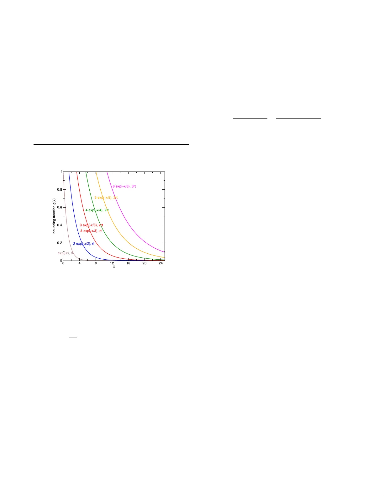
P erf ormance Modeling and Ev aluation for Inf ormation-Driven Netw orks K ui Wu Depar tment of Computer Science Unive rs ity of Victoria B .C. Canada V8W 3P6 wkui@cs.uvic.ca Y uming Jiang, Guoqiang Hu Q2S Center of Excellence Norwegian Univ ersity of Science and T echnology T rondheim, Norway {jiang,gu oqiang.hu}@q2 s.ntnu.no ABSTRA CT Information-driven netw orks include a large category of net- w orking systems, where netw ork no des are aw are of infor- mation delivered and thus can not only forward data pac kets but ma y also p erform information pro cessing. In many si t- uations, the quality of service (QoS) in informatio n- drive n netw orks is provisio ned with the redu ndancy in information. T raditional p erformance mod els generally adopt ev aluation measures suitable for pack et-oriented service guaran tee, such as pack et d elay , t hroughput, and pack et loss rate. These p er- formance measures, ho wev er, do not align well with the ac- tual need of information-driven netw orks. New p erformance measures and models for information-driven netw orks, de- spite th eir imp ortance, h a ve b een mainly blank, largely b e- cause information processing is clearly application dep en- dent and cann ot b e easily captured within a generic frame- w ork. T o fill the v acancy , we present a new performance ev aluation framewo rk particularly tailo red for information- driven net wo rks, based on the recent develo pment of stochas- tic netw ork calculus. W e analyze the QoS with respect to information delivery and stu dy the scheduling p roblem with the new p erformance metrics. Our analytical framew ork can b e used to calculate the netw ork capacity in information de- liv ery and in the mean time to help transmission scheduling for a large b ody of systems where Q oS is sto c hastically guar- anteed with the red u ndancy in information. Categories and Subject Descriptors C.4 [ Performance of Systems ]: Mo deling techniques; H.1 [ Mode ls and Principles ]: Miscellaneous General T erms Theory , Performance Keyw ords Netw ork Calculus, Information-Driven Net works, Perf ormance Modeling 1. INTR ODUCTION Although computer netw orks in general are purp osed for information d eliv ery , most existing n et work architectures lik e the Internet are actually not information driv en in t he sense that netw ork no des (e.g., routers and switchers) only care about p ackets instead of the information inside. As a common principle, netw ork no des as well as th e whole netw ork system are designed to supp ort quality of service (QoS) with resp ect to p ac ket-orien ted service measures suc h as b ound ed pack et d ela y and promised data throu gh p ut. T o achiev e this, QoS provisio ning mechanisms [3] hav e b een prop osed and used in the Internet, includ in g admission con- trol, congestion con trol, resource reserv ation, QoS routing, and so on. It h as b een observed that on the one hand QoS provisi oning mec hanisms pro vide certain serv ice guaran tee to privileged data traffic; on the other hand they largely in- crease the system complexit y and incur a h ea vy burden o n netw ork nod es. Many emerging netw ork systems, for exam- ple, wireless sensor netw orks, consist of no des with only very limited computational capabilit y and th us d o not ha ve the luxury to accommo date complex QoS mec hanisms. Nev- ertheless, Q oS is imp ortant in any means. F or instance, in a p atien t-monitoring system or a fi re alarm system with wireless sensor netw orks, we certainly require imp ortant in- formation like abnormal h eart b eats or high temp erature readings to b e delive red correctly to a monitoring center. The d ilemma w e face is to guarantee QoS mayb e without any un derlying promise from netw ork no des on timely p er pack et delivery . The traditional meaning of Q oS, e.g., for guaranteed p er pack et delivery and end-to-en d delay , is actually an o verkill, since all w e care is information. The traditional solutions fo- cusing on pack ets instead of the information inside ha ve the historical reason: the netw ork proto col stac k is la yered and netw ork proto cols should not mix up with app lication-la yer information. With the emergence of new tec hnologies such as wireless sensor n et works, h o wev er, t h e la yering principle is not necessarily a rule of thum b, and the red undancy in the information sources should be utilized in netw ork pro- tocol design. A netw ork nod e may not b e purely a data forw arding device. Instead, it ma y b ecome aw are of infor- mation forw arded and is able to p erform information pro- cessing whenever necessary . The ultimate goal of the whole netw ork system is no longer to guarantee service for indi- vidual pack ets, but to guarantee a certain amount of i nfor- mation to b e successfully transp orted. W e call this typ e of netw orking systems information-driven networks . T yp i- cal examples include wireless sensor netw orks with directed Figure 1: A simple e xample of wireless s ensor net- wor ks data diffu sion [10], distributed conten t sharing o ver p eer-to- p eer netw orks [2, 12], and netw ork s using netw ork coding [1, 26]. Making the n et work to be information driv en op ens sp e- cial opp ortunities for QoS p rovisioning, e.g., in environmen t where the net work is sub ject to high pac ket losses or net- w ork no des are stringently constrained by computational p o wer and limited bandwidth. In applications where data exhibit spatial and/or temp oral correlation, it is unnecessary to pro vide reliable transmission for each ind ividual pack et. Instead, QoS is guaran teed as long as req uired information can b e obtained as sure (i.e., with a very high probabilit y). W e u se a simple example to illustrate th e adv antages of al- lo wing the netw ork to b ecome information aw are. Example 1. Assume that a wir el ess sensor network in- cludes six sensor no des and one pr o c essing c enter, al so c al le d the sink no de, as shown in Fi gur e 1. F our sensors at the b ot- tom of the figur e monitor the envir onment and p erio di c al ly send out me asur ement data like temp er atur e, humidi ty r e ad- ings. Two sensors in the midd le of the figur e ar e use d as data r elay to the sink. W ir eless links ar e gener al ly subje ct to a high loss r ate i n wir eless sensor networks [23], so we assume that the aver age p acket l oss r ate is 25% for e ach wir eless link. Without c onsidering i nformation, we tr e at the network as pur el y a data delivery system li ke the Internet. In this c ase, we ne e d to make sur e that e ach data p acket is c orr e ctly deliver e d f r om the sour c e t o t he sink with a high pr ob abili ty. If we set this pr ob abil i ty to b e no smal ler than 96% , we ne e d ab out 24 tr ansmissions in total (c al culate d with two r etr ans- missions e ach link to guar ante e the high pr ob abil ity of c orr e ct end-to-e nd p acket delivery). In c ontr ast, i f r elay no des know that the information fr om the four sour c e sensors is highly c orr elate d and i f the i nformation is c onsider e d to b e deliver e d as long as at le ast one p acket fr om the sour c es is r e c eive d by the sink, eight tr ansmissions (e.g., without any r etr ansmi s- sions) c an guar ante e that the information is deliver e d with a pr ob abil ity no smal ler than 96% . The ab o ve example clearly illustrates th e necessity of t ak- ing information in to consideration. Y et, sev eral difficulties need to address even in the very simple example. First, how can w e capture and mo del the correlation at the in- formation sources? In addition, t h e correlation may change o ver time. How can we capt ure the dyn amic changes in a timely fa shion? Second, the above example only consid- ers the correlation at the informatio n sources, h ow can we p erform information p rocessing at intermediate rela y no des for b etter QoS provisioning and resource saving? Third, the use of app lication-la yer information in netw ork protocols has changed the fundamental design principle of current Inter- net architecture, where the n et work is considered as a pack et transp ortation to ol and the service guarantee is promised for individual pack ets. This fund amental change renders t radi- tional performance mo deling and ev aluation approac hes in- v alid for information-driven netw orks. F or instance, netw ork throughput in terms of number of bits p er time unit and end- to-end pack et dela y are no longer go od measures and new metrics sh ou ld be used to align with t he need of information- driven netw orks. What should b e a go od model for p erfor- mance ev aluation and resource sc h eduling for informa tion- driven netw orks? During t he last severa l years, th ere are substantial re- searc h efforts devoted to tackling the first t wo difficulties. P articularly , the spatial and temp oral correlations of infor- mation hav e b een stud ied and utilized in netw ork sc hed uling and resource sa ving in wireless sensor n et works [18, 20, 24]; information red undancy has been exploited to help load bal- ancing and impro ve fault tolerance in p eer-to-p eer con tent sharing systems [2, 12]. Regarding the th ird c hallenge, to the b est of our knowl edge, the only attempts to accommo- date information processing in p erformance mo deling are the w ork in [8, 21]. Nevertheless, information pro cessing is sim- ply mo d eled with a scaling function in [8, 21] and the infor- mation embedd ed in data pack ets h as not b een mod eled, let alone utilized. In this sense, the p erformance mod els in [8, 21] are not reall y informa tion-d riv en mo dels. A systematic p erformance modeling framew ork suitable for informati on- driven netw orks still remains largely op en. In this pap er, w e prop ose the first- of-the-kind analyti- cal framew ork suitable for performance stu dy and resource sc hedu ling of information-drive n netw ork s. Particularl y , we make th e follo wing contributions: 1. W e present a comprehensive p erformance mod el for information-drive n n et works based on the recent de- velo pment of sto c hastic netw ork calculus. Particularly , our mo del captu res the information correlation and the QoS guarantee with respect to sto chas tic information delivery rates, whic h ha ve never b een formally mo d- eled b efore. 2. W e study the sto c hastically achiev able netw ork capac- it y in information delivery and deriv e the b ounds on probabilit y of information delive ry within a given end - to-end information dela y . 3. W e study the transmission sc heduling problem in in- formation - driven n et works and design algorithms to searc h for feasible transmission schedules to meet given QoS requirements. 4. W e give examples to illustrate how our analytical frame- w ork can b e used to solve problems in practice. The rest of the pap er is organize d as follo ws. Section 2 includes the background kno wledge on stochastic netw ork calculus. In Sections 3 and 4, w e present a calculus and a system model for information-driven netw orks, respectively . W e analyze the sto c hastically achiev able information deliv- ery rates in Sections 5, and study th e transmission sc hedul- ing problem in S ection 6. W e present the numerical ex per- iment res ults in Section 7. I n Section 8 we answ er seve ral common q uestions on i nformation-driven n et work calculus, and in Section 9 we introduce related work. The pap er is concluded in Section 10. 2. B A CKGROUND OF ST OCH ASTIC NET - WORK CALCUL US 2.1 Notation W e first introdu ce the notation and key concepts of stochas- tic netw ork calculus [11, 17]. Throughout this pap er, we assume that all arriv al curves and service curv es are non- negative and wide-sense increasing functions. F ollowing the conv ention, w e use A ( t ) and A ∗ ( t ) to denote the cumulativ e traffic arrives and dep artures in time interv al (0 , t ], respec- tively , and use S ( t ) to denote the cu m ulative amount of service provided by the system in time interv al (0 , t ]. F or any 0 ≤ s ≤ t , w e denote A ( s, t ) ≡ A ( t ) − A ( s ) , A ∗ ( s, t ) ≡ A ∗ ( t ) − A ∗ ( s ) , and S ( s, t ) ≡ S ( t ) − S ( s ) . W e adopt A (0) = A ∗ (0) = S (0) = 0. W e denote by F the set of non-negative wide-sense in- creasing funct ions, i.e., F = { f ( · ) : ∀ 0 ≤ x ≤ y , 0 ≤ f ( x ) ≤ f ( y ) } , and by ¯ F the set of non-negative wide-sense decreasing fun c- tions, i.e., ¯ F = { f ( · ) : ∀ 0 ≤ x ≤ y , 0 ≤ f ( y ) ≤ f ( x ) } . F or any random va riable X , its distribution function, de- noted by F X ≡ P r ob { X ≤ x } , b elongs t o F , and its comple- mentary distribution fun ction, denoted by ¯ F X ≡ P rob { X > x } , b elongs t o ¯ F . 2.2 Operators The follo wing op erations defined u nder the (min , +) alge- bra [4, 7, 16] will b e used in t h is pap er: • The (min , +) c onvolution of functions f and g is ( f ⊗ g ) ( t ) = inf 0 ≤ s ≤ t { f ( s ) + g ( t − s ) } . (1) • The (min , +) de c onvolution of functions f and g is ( f ⊘ g )( t ) = sup s ≥ 0 { f ( t + s ) − g ( s ) } . (2) • The (min , +) inf -sum of functions f and g is: ( f ⊙ g ) ( t ) = inf s ≥ 0 { f ( t + s ) + g ( s ) } . (3) 2.3 Per formance Measur es, T raffic a nd Server Models The follo wing measures are of interest in service guarantee analysis u nder netw ork calculus: • The backlog B ( t ) in the system at time t is defin ed as: B ( t ) = A ( t ) − A ∗ ( t ) . (4) • The dela y D ( t ) at time t is defined as: D ( t ) = inf { τ ≥ 0 : A ( t ) ≤ A ∗ ( t + τ ) } . (5) Sto c hastic arriv al curve and sto chastic service curve are core concepts in stochastic netw ork calculus with the for- mer for traffic modeling and th e latter for server modeling. It is worth noting th at the deterministic arri va l cu rv e traf- fic model and th e deterministic service curve server model under (d eterministic) n etw ork calculus are a sp ecial case of their co rresp onding stochastic d efinition. In the literature, there are several definition v ariations of sto chastic arriv al curve and sto c hastic service curve [11] such as: Definition 1. A flow A ( t ) is said to hav e a maximum- virtual-b acklo g-c entric sto chastic arrival curve α ∈ F with b ounding function f ∈ ¯ F , denot e d by A ∼ m.b.c. < f , α > , iff for al l t ≥ 0 and al l x ≥ 0 , ther e holds [11] P r ob { sup 0 ≤ s ≤ t sup 0 ≤ u ≤ s [ A ( u, s ) − α ( s − u )] > x } ≤ f ( x ) . (6) Definition 2. A server i s said to pr ovide a flow A ( t ) with a sto chastic servic e curve β ∈ F with b ounding function g ∈ ¯ F , denote d by S ∼ s.c < g , β > , iff f or al l t ≥ 0 and al l x ≥ 0 , ther e holds [ 11] P r ob { sup 0 ≤ s ≤ t [ A ⊗ β ( s ) − A ∗ ( s )] > x } ≤ g ( x ) . (7) With the ab ov e definitions and their v ariations, v arious prop erties of sto chastic netw ork calculus, including sto chas- tic bac klog an d stochastic dela y bounds, hav e been pro ved (e.g., see [11, 17]). 3. AN INFORMA TION-DRIVEN NETWORK CALCULUS 3.1 Notation on Information T raditional sto chastic netw ork calculus uses the traffic ar- riv al curve and the service curve to count for cumulativ e amount of traffic or service. If netw ork n odes are informa- tion driven and can p erform in-netw ork pro cessing, we need a translation from t he amount of traffic to the amount of information in order to mo del information processing at net- w ork nodes. W e hence develop a stoc hastic net work calcu- lus dedicated to p erformance mo deling of information-driven netw orks. Although entrop y (or entrop y rate) is broadly used to measure information of random var iable (or rand om pro- cess) [6], to avo id v arious details in entrop y estimation in sp ecific applications [15], w e simply use th e notation H ( A ( t ) ) to denote the information of A ( t ) b ut lea ve its pr actic al me aning and c al cul ation op en to users . Nevertheless, w e need to define basic p roperties of information to mak e f ur- ther analysis p ossible. Definition 3. The information of a flow A ( t ) is denote d as H ( A ( t )) and has th e fol lowing pr op erties: 1. H ( ∅ ) = 0 wher e ∅ denotes t he nul l set; H ( A (0)) = 0 . 2. H ( A ( t )) i s a non-ne gative, non-de cr e asing function of time t , and for ∀ t and 0 ≤ s ≤ t , H ( A ( t )) = H ( A ( s )) + H ( A ( s, t )) holds for the same flow, i.e., the flo w fr om the same information sour c e. 3. F or differ ent flo ws A i ( t ) , i = 1 , . . . , N , N X i =1 H ( A i ( t )) ≥ H ( N X i =1 A i ( t )) , (8) wher e P N i =1 A i ( t ) me ans the sup erp osition of flows A 1 ( t ) , . . . , A N ( t ) . The first prop erty of information means that the infor- mation of a flow is initially zero. The second one means that the information of a fl o w do es not become smaller as more data arrive and th e information from the same fl o w is accumula tive, i.e., H ( A ( s, t )) should be u nderstoo d as the new information in the flow at time interv al ( s , t ]. The third prop ert y means that the sup erp osition o f different flows do not increase the total information in the fl ows. Note that these t hree prop erties are consis tent with the entrop y defi- nition. F or ease of exp osition, we omit th e time index whenever doing so will not cause confusion. Definition 4. R e dundant i nformation is a me asur e of the information r e dundancy i n di ffer ent flows, A 1 , . . . , A N . It is define d i n this p ap er as I ( A 1 ; . . . ; A N ) ≡ N X i =1 H ( A i ) − H ( N X i =1 A i ) , (9) and has the f ol lowing pr op erties: 1. If A 1 , . . . , A N ar e indep endent, I ( A 1 ; . . . ; A N ) e quals 0 . 2. F or any i (= 1 , . . . , N ) , I ( A 1 ; . . . ; A N ) ≤ H ( A i ) . Definition 5. Information of a set of data sour c es A = < A 1 , . . . , A M > , H ( A ) , i s define d as H ( A ) ≡ H ( M X i =1 A i ) = M X i =1 H ( A i ) − I ( A 1 ; . . . ; A M ) (10) 3.2 Modeling Flow and Service with Respect to Inf ormation Definition 6. A flow A ( t ) is said to have an information sto chastic arrival curve α ∈ F with b ounding function f ∈ ¯ F , denote d by A ∼ i.s.a. < f , α > , iff for al l t ≥ 0 and al l x ≥ 0 , ther e holds P r ob { sup 0 ≤ s ≤ t sup 0 ≤ u ≤ s [ H ( A ( u, s )) − α ( s − u )] > x } ≤ f ( x ) . (11) Definition 7. A flow A ( t ) is said to have an lower - b ounde d i nf ormation sto chastic arrival curve γ ∈ F with b ounding function θ ∈ F , denote d by A ∼ l.i.s.a < θ , γ > , iff for al l t ≥ 0 and al l x ≥ 0 , ther e holds P r ob { inf 0 ≤ s ≤ t inf 0 ≤ u ≤ s [ H ( A ( u, s )) − γ ( s − u )] ≤ x } ≤ θ ( x ) . (12) Definition 8. A server i s said to pr ovide a flow A ( t ) with an information sto chastic servic e curve β ∈ F with b ounding function g ∈ ¯ F , denote d by S ∼ i.s.s. < g , β > , iff for al l t ≥ 0 and al l x ≥ 0 , ther e holds P r ob { sup 0 ≤ s ≤ t [ H ( A ( s )) ⊗ [ β ] x ( s ) − H ( A ∗ ( s ))] > x } ≤ g ( x ) (13) wher e [ β ] x ( t ) ≡ max { β ( t ) , x } . time H (A(t))/H(A * (t)) H (A(t)) H (A * (t)) t t+ τ D(t) B(t) B(t, τ ) Figure 2: The illustration of performance measures Note that information service i nclud es b oth i nformation processing and information transmissio n. W e also use the terms i nformation servic e r ate a nd i nformation arrival r ate : Definition 9. The (aver age) information servic e r ate of a server fol lowing ∼ i.s.s. < g , β > is define d as l im t →∞ β ( t ) t . Definition 10. The (aver age) i nformation arrival r ate of a flow f ol lowing ∼ i.s.a. < f , α > is define d as lim t →∞ α ( t ) t . In th e rest of the p aper, unless otherwise men tioned, ser- vice by default is referred as information service. 3.3 Per formance Measur es The follo wing d efinitions are used for in formatio n guaran- tee analysis: Definition 11. The information delay of input flow A ( t ) in a system at time t is define d as : D ( t ) = inf { τ ≥ 0 : H ( A ( t ) ) ≤ H ( A ∗ ( t + τ )) } , (14) wher e A ∗ ( t ) is the output flow. Definition 12. The information b acklo g at time t in a system is define d as: B ( t ) = H ( A ( t )) − H ( A ∗ ( t )) , (15) wher e A ( t ) and A ∗ ( t ) ar e input flow and output flow, r esp e c- tively. Definition 13. The inf ormation b acklo g wi thin delay b ound τ ( ≤ D ( t )) at time t i s define d as: ˆ B ( t, τ ) = H ( A ( t )) − H ( A ∗ ( t + τ )) . (16) T o help b etter understand ing, Figure 2 illustrates the ab ov e three defin itions. 3.4 Basic Prope rties of Inf ormation-Driven Net- work Calculus T o make t h e pap er concise and easy to follo w, w e pu t all proofs in A pp endix A. Lemma 1. [11] F or any r andom variables X and Y , and ∀ x ≥ 0 , if ¯ F X ( x ) ≤ f ( x ) and ¯ F Y ( x ) ≤ g ( x ) , wher e f , g ∈ ¯ F , then P r ob { X + Y > x } ≤ ( f ⊗ g )( x ) . (17) Lemma 2. F or any r andom variables X and Y , and ∀ x ≥ 0 , if ¯ F X ( x ) ≤ f ( x ) and F Y ( x ) ≤ g ( x ) , wher e f ∈ ¯ F , g ∈ F , then P r ob { X − Y ≥ x } ≤ ( f ⊙ g )( x ) . (18) Theorem 1. (Sup erp osition) C onsider two flows A 1 ( t ) and A 2 ( t ) . L et A ( t ) denote the ag gr e gate flow, i.e., A ( t ) = A 1 ( t ) + A 2 ( t ) . If for b oth flows A i ∼ i.s.a. < f i , α i >, i = 1 , 2 , and I ( A 1 ; A 2 ) ∼ l.i.s.a. < θ , γ >, then A ∼ i.s.a. < f , α >, wher e f ( x ) = ( f 1 ⊗ f 2 ⊙ θ )( x ) , and α ( t ) = α 1 ( t ) + α 2 ( t ) − γ ( t ) . Theorem 1 means that if tw o flow s follow i.s.a. curves, their information fusion (i.e., flo w aggregation with information redundancy remov ed) also follo ws an i.s.a. curve. Theorem 2. (Conc aten ation) Consider a flow A ( t ) p ass- ing thr ough a net work of N no des in tandem. If e ach no de pr ovides servic e S i ∼ i.s.s. < g i , β i >, i = 1 , 2 , . . . , N , then the network guar ante es to the flow a servic e S ∼ i.s.s. < g , β > with β ( t ) = β 1 ⊗ . . . ⊗ β N ( t ) g ( x ) = g 1 ⊗ . . . ⊗ g N ( x ) . Theorem 2 ind icates th at the service provided by an end-to- end path follo ws an i.s.s. curve if the nod es along the p ath follo w i.s.s. curves. Theorem 3. (Output) Consider a no de with input flow A . If A ∼ i.s.a. < f , α > , and the no de pr ovides the flow with servic e S ∼ i.s.s. < g , β > , then the output A ∗ ∼ i.s.a. < f ⊗ g , α ⊘ β > . Theorem 3 means that the inp ut flow and the output fl ow b oth follo w i.s.a. curve s, if the service no de follo ws an i.s.s. curve. The follo wing th eorem illustrates the service guarantee provided by a netw ork n ode in terms of information backlog, information delay , and information backlog within a dela y b ound. Theorem 4. (Service guar an te e) I f the i nput flow has A ∼ i.s.a. < f , α > , and the networ k no de pr ovides the flow with servic e S ∼ i.s.s < g , β > , then 1. The information b acklo g B ( t ) of the flow at time t sat- isfies: for al l t ≥ 0 and al l x ≥ 0 , P r ob { B ( t ) > x } ≤ f ⊗ g ( x − α ⊘ β (0)) . (19) 2. The information delay D ( t ) of the flow at time t sat- isfies: for al l t ≥ 0 and al l x ≥ 0 , P r ob { D ( t ) > h ( α x , [ β ] x ) } ≤ f ⊗ g ( x ) , (20) wher e α x ( t ) ≡ α ( t ) + x , [ β ] x ( t ) ≡ max { β ( t ) , x } , and h ( α, β ) i s the maximum horizontal distanc e b etwe en functions α and β and is define d as h ( α, β ) = sup s ≥ 0 { inf { τ ≥ 0 : α ( s ) ≤ β ( s + τ ) }} . 3. The inf ormation b acklo g wi thin delay b ound τ ( ≤ D ( t )) of the flow at time t satisfies: for al l t ≥ 0 and al l x ≥ 0 , P r ob { ˆ B ( t, τ ) > x } ≤ f ⊗ g ( x + inf v ≥ 0 [ β ( v ) − α ( v − τ )]) . (21) Note that α ( t ) = 0 for t ≤ 0 . Figure 3: The architecture of i nformation-dr iven netw orks 4. SYSTEM MO DEL OF INFORMA TION- DRIVEN NETWORKS The architecture of informatio n- driv en netw orks is illus- trated in Figure 3, includ ing information sources, th e trans- p ortation paths, and the information destination (or t he sink). T o simplify presentati on, w e only consider one sink nod e. The mo d el, h o wev er, could b e easily extended to mul- tiple information sinks. 4.1 The Model for In formation Sour ces Assume t hat there are M information sources in the sys- tem, denoted as A 1 , A 2 , . . . , A M , respectively . W e assume that an info rmation source A i ( i = 1 , . . . , M ) has a certain amount of information to send to the destination. W e de- note th e traffic sent from A i as A 0 i ( t ) and t h e traffic finally arriv es at the d estination as A h i i ( t ), where h i is the num b er of hops of the path used for the information deliv ery from A i to the d estination. F or the M information sources, w e use I ( A 0 i ( t ); . . . , A 0 j ( t )), 1 ≤ i < j ≤ M to model the information red u ndancy among different d ata sources. 4.2 The Model for T ransportation Paths W e assume that K path s, denoted as L 1 , . . . , L K , from the set of information sources to the d estination are used for in- formation deliv ery . In this pap er, we only fo cus on K paths that are nod e-disjoin ted. When m ultiple paths share some common intermediate no des, the num b er of p ossible schemes for information fusion b ecomes t remendous, in which case it is extremely difficult to derive the p erformance b ounds. W e lea ve the study of m ultiple paths sharing in termediate nod es as our futu re w ork. N ev ertheless, w e do n ot assume the data transmissions a long the K paths are alwa y s inde- p endent. F or ex ample, in wireless netw orks even if tw o paths do not share common intermediate n odes, t he transmissions along the tw o paths may in terfere with eac h other. In short, w e assume that t he t ran smissions along different paths ma y impact each other, but information fusion is only p erformed at t h e entrance n odes and the sink no de. As a reminder, the information service in Defin ition 8 includes b oth information processing and information transmission. In addition, w e assume that an end- t o-end path , once es- tablished, is fixed for the time p erio d of interest. Netw orks in which an end-to-end p ath changes quickly ov er time are b ey ond th e focus of this pap er and are left as our future w ork. W e denote a p ath L i of length h i (i.e., the hop count from the source to the destination is h i ) as L i = ( L 0 i , L 1 i , . . . , L h i i ), where L j i denotes the j -th no de of path i . Each no de L j i provides an info rmation stochastic service curve S ∼ i.s.s < g j i , β j i > along the path . When tw o paths, L i = ( L 0 i , L 1 i , . . . , L h i i ) and L j = ( L 0 j , L 1 j , . . . , L h j j ) interf ere with each other in data transmission, w e define an h i × h j matrix [ ˆ I ( l,m ) ] , l = 0 , . . . , h i − 1 , m = 0 , . . . , h j − 1 to capture the transmission correlation along the t wo paths, where ˆ I ( l,m ) is an information impairment process t hat should b e integrated in the information service curves of the no des L l i and L m j . This information impair- ment p rocess is in tro duced to redu ce the information service rate along the paths inv olved. N ote th at L h i i = L h j j since w e assume the same d estination. T o inv estigate th e impact of transmission interf erence, the follo wing theorem will b e used to adjust the service rate of an impacted no d e. Its pro of is pro vided in App endix A. Theorem 5. (Service r e duction with i nformation i m- p ai rment) Consider a network no de pr oviding a flow with servic e S ∼ i.s.s. < g , β > . If the no de is interfer e d with an imp airment pr o c ess ˆ I with information sto chastic arrival curve ˆ I ∼ i.s.a. < f , α > , then the network no de guar ante es to the flow a s ervic e S ∼ i.s.s. < g ⊗ f , β − α > . 4.3 Prob lems of Inter est Thus far, we hav e presented a calculus and an abstract mod el for information-driven netw orks. Among many inter- esting problems in this analytical framew ork, w e are in ter- ested in the follo wing key questions: 1. What are the sto c hastically ac hiev able information de- liv ery rates of a n etw ork? The answ er to the question discloses the limit of information delivery in the sys- tem. 2. Given a set of information sources and an end -to-end dela y b ound, can the total information b e delivered to the destination with a h igh probabilit y , and ho w? The answ er to the question provides insights on the design of scheduling algorithm for information-driven netw orks. In th is paper, we focu s only on th e feasibilit y of infor- mation deliv ery and p erformance b ounds, but in tentionally a void th e study of man y in teresting optimiza tion problems within t h e analytical framewo rk. This is because the main purp ose of this pap er is to p resen t a n ew analytical app roac h and its application for information-driven n et works and also b ecause traditional measuremen ts on resource ove rhead hav e not b een w ell defin ed in informati on-d riv en netw orks. F or instance, w e need to math ematicall y form ulate the compu- tational ov erhead for information pro cessing. W e leav e these aspects as our future work. 5. STOCHASTICALL Y A CHIEV ABLE INFOR- MA TION DELIVER Y W e answ er the first question in this section. F or this, w e need to inv estigate the information service gu arantee p ro- vided by m ultiple serv ers in p aralle l, as shown in Figure 4 . F or simplicit y , we assume a flu id mo del in which information could b e split in infin itesimal amounts. This constraint will b e relaxed in the next section. S ~i.s.s. < g 1 , β 1 > S ~i.s.s. < g 2 , β 2 > S ~i.s.s. < g N , β N > A(t) A 1 (t ) A 2 (t ) A N (t ) Splitte r A * (t ) Figure 4: An i nformation spl itter for servers in par- allel Definition 14. A weighte d information splitter is a sche d- uler that splits an input flow A ( t ) into multiple inf orma- tion exclusive sub-flows A 1 ( t ) , . . . , A N ( t ) , wi th e ach assigne d a weight w i and serve d by an information pr o c essing no de S i ( i = 1 , . . . , N ) , r esp e ctively. A t any time instant t , the sub-flow assigne d to S i satisfies H ( A i ( t )) = w i P N j =1 w j H ( A ( t )) . Theorem 6. (Par al lel servers) Consider a flow A ( t ) p assing thr ough a weighte d i nformation splitter and then a network of N no des in p ar al lel (Figur e 4). Assume that al l no des ar e work c onserving, i.e., they c annot b e c ome i d le if ther e is information waiting for servic e. Assume that e ach no de pr ovides servic e S i ∼ i.s.s. < g i , β i > ( i = 1 , 2 , . . . , N ) and the weight of the sub-flow to S i at time t i s set to β i ( t ) . The whole system guar ante es to the flow a servic e S ∼ i.s.s. < g , β > with β ( t ) = ( β 1 + . . . + β N )( t ) g ( x ) = g 1 ⊗ . . . ⊗ g N ( x ) . It is worth highligh ting that Theorem 6 is intended to dis- close a netw ork’s ac hiev able informa tion delivery rate, and for this reason it assumes an ideal situation in whic h infor- mation could b e split in infin itesimal amounts. In practice, how ever, such an assumption may not hold and t h e net- w ork’s actual information delivery rate would b e lo wer. Equipp ed with the theorems in this p aper, Algorithm Rate- Cal, sho wn in Figure 5, can b e used to searc h for stoc has- tically ac hieva ble information deliv ery rates of a netw ork. It uses a brutal-force search and has a time complexity of O (2 K ), where K is the num b er of no de-disjoint paths from the sources to the d estination. The algorithm is not scal- able with K , b ut practically K is usually not very large. In addition, it is very easy to reduce th e complexity by con- sidering the sto chas tic relationship of i.s.s. curve s. A curve S 1 ∼ i.s.s. < g 1 , β 1 > is considered b etter th an another curve S 2 ∼ i.s.s. < g 2 , β 2 > iff for ∀ t , x ≥ 0, β 1 ( t ) > β 2 ( t ) and g 1 ( x ) ≤ g 2 ( x ). I n this case, we can ignore the curv e S 2 to reduce the searc h space. Example 2. We use a si mple example to il lustr ate the c al culation of sto chastic al ly achievable information deli very r ates of a network. Assume that a network has thr e e p ar- al lel end-to-end p aths, L i , i = 1 , 2 , 3 . Assume that p ath L i includes i (= 1 , 2 , 3) no des, r esp e ctively. Assume that the tr ansmissions along differ ent p aths do not interfer e with e ach other. Also assume that al l no des pr ovide the same inf or- mation sto chastic servic e fol lowing ∼ i.s.s. < e − x , r t > . Run - ning Algor ithm R ateCal, we obtain seven i. s.s. curves, as Input: A netw ork with K parallel paths (Figure 4); i.s.s. curve of eac h no de; A set of impairment matrices; Output: a list of sto chastica lly achiev able services; Metho d: 1: FOR any subset of the K paths, { L i , . . . , L j } , where 1 ≤ i ≤ j ≤ K { 2: FOR n = i TO j { 3: FOR each no de along path L n , if its transmission is interfered by another path in the subset, 4: Adjust th e nod e’s i.s.s. with Theorem 5 and the i. s.a. curves in releva nt impairment m atrices; 5: Calculate the i.s.s. of path L n with Theorem 2; } 6: Output the i .s.s. of subset { L i , . . . , L j } with Theorem 6; } Figure 5: R ateCal : An algorithm to calculate stochastically achiev abl e i nformation delivery rates. Figure 6: Stochastically a c hiev able servi ce curves in the example netw ork shown in Figur e 6. F or instanc e, b ase d on the i.s.s. curve < 6 e − x/ 6 , 3 rt > , we c an se e that for a (deterministic) infor- mation arrival fol l owi ng ∼ i.s.a. < 0 , 3 r t > , the networ k c an guar ante e its delivery such that up to tim e t , the pr ob abil ity that the output information i s less than 3 r t − 24 i s smal ler than 0 . 1( ≈ 6 e − 24 6 ) . 6. TRANSMISSION SCHEDULING Although the prev ious section pro vides the answ er to stochas- tically ac hiev able information delivery rates, the results are based on an ideal assumption, that is, the information could b e spli t in infinitesimal amo unts. In practice, ho wev er, w e are often met with th e situation th at information cannot b e split arbitrarily . In th is sense, th e results of previous section only provide theoretical upp er b ounds on sto c hastic infor- mation deliv ery rates, which may not b e practically feasible for a giv en request. W e hence need to stu d y t he fo llowi ng problem: Giv en a set of information sources and an end-to- end delay b ound, can th e total information b e delivered to the destination with a high probability (e.g. n o lesser than p )? If yes, how? if not, what is the p ercen tage of th e infor- mation that could b e d eliv ered and in what probability? Definition 15. A tr ansmission sche dule for a set of in- formation sour c es A = < A 1 , . . . , A M > over a s et of p aths L = < L 1 , . . . , L K > is denote d as a tuple < A, L, π > , wher e π is a mapping function fr om A to L , and π ( A i ) = L j me ans that data fr om sour c e A i (1 ≤ i ≤ M ) is sent over p ath L j (1 ≤ j ≤ K ) in the t r ansmission sche dule. Definition 16. Information delivery r atio within delay τ : F or a set of information sour c es A = ( A 1 , . . . , A M ) sent fr om M sour c es to a destination, the inf ormation delivery r atio at time t , R ( t ) , is define d as R ( t ) ≡ H ( A ∗ ( t + τ )) H ( A ( t )) = H ( A ( t )) − ˆ B ( t, τ ) H ( A ( t )) , (22) wher e A ∗ ( t + τ ) r epr esents the set of tr affic that has arrive d at the information sink at t im e t + τ . The scrut in izing readers may h a ve realized th at H ( A ∗ ( t + τ )) is n ot wel l defin ed b ecause to get it needs calculation of I ( A ∗ 1 ; . . . ; A ∗ M ), which has not b een defi ned. The follo w- ing theorem d isclose s t he relationship of information redun- dancy b efore and after information delive ry and can b e used to ov ercome this difficulty . Theorem 7. Consider a set of inf ormation sour c es A = ( A 1 , . . . , A M ) . Spli t the set into two subsets ∆ 1 = ( A 1 , . . . , A i ) and ∆ 2 = ( A i +1 , . . . , A M ) , and tr ansmit ∆ 1 and ∆ 2 simul- tane ously along two sep ar ate p aths at time t . Assume that at time t + τ , b oth H (∆ 1 ) and H (∆ 2 ) have b e en r e c eive d, i.e., H (∆ ∗ 1 ( t + τ )) = H (∆ 1 ( t )) and H (∆ ∗ 2 ( t + τ )) = H (∆ 2 ( t )) . We have I ( ∆ ∗ 1 ( t + τ ); ∆ ∗ 2 ( t + τ )) = I (∆ 1 ( t ); ∆ 2 ( t )) . Note that Theorem 7 holds no matter whether the infor- mation redundancy wi thin e ach set ∆ i , i = 1 , 2 is remo ved or not during the transmission. With D efinitions 15 and 16, the formal formulatio n of the problem b ecomes: Given a set of information sources A = ( A 1 , . . . , A M ), a set of separate transportation paths L 1 , . . . , L K , an end-t o- end delay b ound D , and a proba- bilit y p , is there a transmission schedule to deliv er the in- formation from the sources to the destination within time dela y D with a probabilit y n o smaller th an p ? I t is easy to see that this problem is NP- hard even without consid- ering the information redu n dancy among the information sources, b ecause the problem can b e transformed into a “bin- packing” p roblem [9 ], which is N P-hard. W e h ence prop ose a method , called b est-fit- largest-redun dancy(BFLR) algo- rithm, to searc h for an appro ximate solution. An error may occur if the algorithm return s a negativ e answer to the ex- istence of a feasible transmission schedule, but a feasible transmission schedule d oes actu ally exist. N ev ertheless, d ue to the NP-h ardn ess of t h e problem, such an error cannot b e av oided u nless b oth K and M are very small so that we can use b rutal-force search. Our later exp erimen tal stud y sho ws that BFLR can find almost all feasible transmission sc hedu les. The basic idea of the BFLR algorithm is t o use the sto c has- tically achiev able serv ice rates obtained by Algorithm Rate- Cal as the guideline in the s election of a feasible subset of paths, and com bine information sources that hav e the largest information redundancy and can b est fit to a transp ortation path. The detailed step s of BFLR is illustrated in Figure 7. When the BFLR algorithm returns no, it may b e b ecause either (1) the information service rate of a selected path is Input: A netw ork with K parallel paths (Figure 4), each nod e’s service curve, and imp airmen t matrices; A set of in formation sources A = ( A 1 , . . . , A M ) and related information redundancy; End-to-end d ela y b ound D ; The v iolation probabilit y p ; Output: F easible transmission sc hedu les, or no feasible transmission sc hedu le; Metho d: 1: Call A lgorithm RateCal to obtain all stochastically achiev able service rates, each characterized by ∼ i.s.s. < g i , β i > ; 2: Remov e the ac hiev able service rates if its rate is smaller than th e information arriv al rate of H ( A ); 3: Sort the remaining achiev ab le service rates in the decreasing order of rate; 4: Sort A i in the decreasing order of their in formation arriv al rates; //Note: A i ∼ i.s.a. < f i , α i > . 5: FOR each remaining ac hiev able service rate in the sorted order { 6: Find the subset of p aths corresp onding to the current ac hieva ble serv ice rate; // Note: A feasible service rate represents a sub set of p aths. 7: Sort the paths in the decreasing order of th eir service rates; 8: AS = ∅ ; // Note: AS is an in itially empty set to store information sources that could b e combined together. 9: FOR each path in the subset { 10: Find the information source whose information arriv al rate b est fit s the cu rren t path; // Note: Best-fit means that t he source’s informatio n arriv al rate is smaller than th e service rate of th e path, but is t he largest among all non-pro cessed information sources. 11: Use Theorem 4.(2) to chec k if the information source can b e d eliv ered with the cu rrent path to meet the requ iremen t; 12: Go to the next path if b est-fit cannot b e found; 13: Lab el the b est-fit information source as pr o c esse d and insert it into A S ; REPEAT { 14: Find the non-pro cessed information source that has the largest redundancy with AS ; 15: } UNTIL AS cannot b e delivered with the current path to meet the d ela y requ iremen t; 16: IF all information sources ha ve b een p ro cessed, outp ut the transmission sc hedu le; ELSE Go t o the n ext path. } 17: Go to the nex t ac hiev able service rate; 18: Return NO if all ac hiev able service rates h a ve b een chec ked but no feasi ble transmission sc hedule has b een found. 19: } Figure 7: BFLR: An algorithm to searc h for feasibl e transmission sc hedules. smaller than the com bined rate of a subset of sources, or (2) the information service rate of a selected path is larger than the com bined rate of a subset of sources but the information cannot be delivery in the (tight) delay bound. In the first case, no feasible transmission schedule exists even if we en- large the d ela y b ound. In the latter case, the problem that w e n eed to answ er is: what is the information delivery ratio R within the dela y b ound D and in what probability? The problem can be answ ered by revising the BFLR algorithm and using Theorem 4.(3). Basicall y , we should remove Line 18 of the algorithm, and in Line 11 use Theorem 4.(3) to chec k the information bac klog within the dela y boun d and the corresp onding sto chastic b ounding function. I n addi- tion, the out put (Line 16) should b e changed accordingly . W e omit the details to av oid t riv ialit y . 7. CASE STUD Y 7.1 Network Configuration W e use an exemp lary information-driv en n et work t o illus- trate how the results in this p ap er can be used for perfor- mance eva luation in practice. Information sources. W e consider a netw ork consisting of M = 9 information sources. These sources are partitioned into 3 groups with sources 1 ∼ 3 in Group 1, sources 4 ∼ 6 in Group 2, and sources 7 ∼ 9 in Group 3. I nformation from the same group exhibits spatial correlation, but information from different groups is assumed to b e indep endent. T emp oral correlation. Assume that th e information of eac h source is collected by perio dically sampling a stationary Gaussian sto c hastic p rocess. Concretizing th e information H ( · ) of the flow A i generated by source i to the Shannon entrop y function 1 , it yields for discrete time t [6]: H ( A i ( t )) = α i ( t ) = 1 2 log(2 π e ) t |C ( t ) i | , t = 1 , 2 , ... (23) where C ( t ) i is the t × t cov ariance matrix for the flo w of source i and is sp ecified by the temporal co v ariance fun ct ion Γ i ( τ ), i.e., th e matrix element C ( t ) i ( j, k ) = Γ i ( k − j ), where 1 ≤ j, k ≤ t . Here, we adopt the t yp ical exp onential cov ariance function [24]: Γ i ( τ ) = σ 2 i e −| τ | /η i , τ = 0 , ± 1 , ± 2 , ... (24) where σ 2 i is the va riance of flow A i and η i is a constant. Assume that each source generates mess ages at a constant interv al δ . By applying Equation (24) in (23), the sto c hastic arriv al curv e of flow A i can b e specified in th e con tinuous time t as A i ∼ i.s.a. < 0 , α i > , where 1 Shannon’s entrop y function is consistent with our defin ition of information in Section 3.1 α i ( t ) = (25) ( t 2 δ log(2 π eσ 2 i ) , 0 ≤ t ≤ δ t 2 δ log(2 π eσ 2 i (1 − e − 2 /η i )) − 1 2 log(1 − e − 2 /η i ) , t > δ Spatial correlation. In t he same source group, w e mod el the informatio n redu ndancy of t he sources using a spatial correlation mo del similar to that in [24]. Specifically , we assume that for sources in th e same group, H ( X i A i ) = X i ǫ i H ( A i ) , 0 ≤ ǫ i ≤ 1 where ǫ i are constan ts and dep end on the sources ’ lo ca- tions and the adopted spatial model [24]. In our study , we use the same settin g of information redun dancy for all three groups. Sp ecifically , for the three sources in a group, de- noted as A 1 , A 2 , A 3 , we set: H ( A 1 + A 2 ) = H ( A 2 + A 3 ) = H ( A 1 + A 3 ) = 1 . 8 H ( A 1 ) H ( A 1 + A 2 + A 3 ) = 2 . 4 H ( A 1 ) While th e ab o ve parameter settings are k ind of arbitrary , we stress t hat using other p ar ameters has no imp act on the ef- fe ctiveness of our analytic al fr amework since users can adopt any other temporal and spatial correlatio n models different from our example scenario in th eir analysis. 1 1 2 1 2 3 1 2 3 4 sink M=9 sources L 1 L 2 L 3 L 4 Figure 8: An example netw ork T ransportation paths. As shown in Fig. 8, the col- lected information is transmitted to a single information sink through four parallel end-to-end paths, L i , i = 1 , 2 , 3 , 4. On each path L i , th ere are i no des. Assume that all n et- w ork n odes provide information service follo wing ∼ i.s.s. < e − x , r ( t − d ) > , where r is the a verag e information s ervice rate and d is the per-hop delay . Also assume that t he first nod e in L 1 and the first no de in L 2 are sub ject to correlated impairmen t, whic h follo ws ∼ i.s.a. < 4 e − x/ 4 , r ( t − d ) / 5 > . Similarly , assume that the second no de in L 3 and the sec- ond n ode in L 4 are sub ject to correlated impairment, which follo ws ∼ i.s.a. < 3 e − x/ 3 , r ( t − d ) / 3 > . Note that Example 1 is a simplified sp ecial case of this case stu dy . 7.2 Numerical Results W e would lik e to k no w whether t h e information netw ork could deliver th e information from sources to the destination within a given dela y b ound with at least a certain probabil- it y . If feasi ble transmission schedules cannot b e found, w e also w ant to know the information delivery ratio with at least a certain probability . Since the p erformance measures, e.g., delay and informatio n delive ry ratio, are time dep en- dent. we calculate t h eir maximum v alue to remo ve the time T able 1: Information s tochastic se rvice curve of each path P ath w/o impairmen t w/ impairment L 1 < e − x , r ( t − d ) > < 5 e − x/ 5 , 4 5 r t − 4 5 r d ) > L 2 < 2 e − x/ 2 , r ( t − 2 d ) > < 6 e − x/ 6 , 4 5 r t − 9 5 r d ) > L 3 < 3 e − x/ 3 , r ( t − 3 d ) > < 5 e − x/ 5 , 2 3 r t − 8 3 r d ) > L 4 < 4 e − x/ 4 , r ( t − 4 d ) > < 6 e − x/ 6 , 2 3 r t − 11 3 r d ) > dep endancy in t h is case study . F or example, the delay is calculated as sup t ≥ 0 D ( t ). In the example study , we select the rate p arameter r = 8 k bps, per-h op dela y d = 7 . 5 ms. F or every information source, w e set δ = 100 ms and η i = 100. With reference to Equation (25), σ i is set suc h t hat the long-term information rate of a source ≈ 2 . 33 kbps. Considering the spatial corre- lation mo deled, the total long-t erm information arriv al rate of the 9 sources amounts to 16 . 78 k bps. First, w e calculate the in formatio n sto chastic service curve of each path an d list th e results in T able 1. T o facilitate un derstanding, we list the sub sets of paths found b y Algorithm BFLR th at hav e t otal information ser- vice rate larger than t h e total information arriv al rate, i.e., the intermediate result after Step 2 of A lgorithm BFLR: 1. L 1 + L 2 + L 3 ∼ i.s.c. < 14 e − t/ 14 , 13 5 r t − 28 5 r d > 2. L 1 + L 2 + L 4 ∼ i.s.c. < 15 e − t/ 15 , 13 5 r t − 33 5 r d > 3. L 1 + L 3 + L 4 ∼ i.s.c. < 12 e − t/ 12 , 7 3 r t − 22 3 r d > 4. L 2 + L 3 + L 4 ∼ i.s.c. < 13 e − t/ 13 , 7 3 r t − 25 3 r d > 5. L 1 + L 2 + L 3 + L 4 ∼ i.s.c. < 22 e − t/ 22 , 44 15 r t − 134 15 r d > The first item means that if path 1, path 2, and p ath 3 are used, t h e achiev able sto c hastic information service follo ws ∼ i.s.s. < 14 e − t/ 14 , 13 5 r t − 28 5 r d > . The exp lanation of other items is similar. W e can search for feasible transmission schedules u sing Algorithm BFLR for d ifferen t delay b ounds (e.g. 35 ms and 45 ms) and for different v iolatio n probabilities (e.g., P rob = 0 . 001 and P r ob = 0 . 0001). The results are shown in T able 2. In the table, “X” d en otes that the correspondent path set is not feasible. “Ai.j” stands for the source j in Group i . As an example, the fi rst th ree lines on the third column mean t h at if w e send informa tion from sources A 1 . 1 , A 1 . 2 , A 1 . 3 along path L 1 , information from sources A 2 . 1 , A 2 . 2 , A 2 . 3 along path L 2 , and information from sources A 3 . 1 , A 3 . 2 , A 3 . 3 along path L 3 , the total information can b e receiv ed within delay b ound 35 ms with a v iolatio n p robabilit y no larger than 0 . 001. Because information from th e same source group ex- hibits the largest redun dancy , the results d emonstrate th at Algorithm BFLR is capable of finding a transmission sched- ule so that information from th e same source group is fused together to remov e information redundancy . As discussed b efore, when the BFLR algorithm retu rns no, it may b e b ecause either (1) the information service rate of a selected p ath is smaller th an the combined rate of a subset of sources, or (2) the information service rate of a selected path is larger than the combined rate of a subset of sources but the information cann ot b e delivery within the delay b ound. W e fi nd that th e tw o subsets of path s, < L 1 , L 3 , L 4 > and T able 2: Results of BFLR: feasi ble transmissi on sch edul es P r ob / Delay boun d 35 ms 45 ms L 1 : A 1 . 1 ∼ 1 . 3 L 1 : A 1 . 1 ∼ 1 . 3 ( L 1 , L 2 , L 3 ) L 2 : A 2 . 1 ∼ 2 . 3 L 2 : A 2 . 1 ∼ 2 . 3 L 3 : A 3 . 1 ∼ 3 . 3 L 3 : A 3 . 1 ∼ 3 . 3 L 1 : A 1 . 1 ∼ 1 . 3 L 1 : A 1 . 1 ∼ 1 . 3 ( L 1 , L 2 , L 4 ) L 2 : A 2 . 1 ∼ 2 . 3 L 2 : A 2 . 1 ∼ 2 . 3 .1% L 4 : A 3 . 1 ∼ 3 . 3 L 4 : A 3 . 1 ∼ 3 . 3 ( L 1 , L 3 , L 4 ) X X ( L 2 , L 3 , L 4 ) X X L 1 : A 1 . 1 ∼ 1 . 3 ( L 1 , L 2 , L 3 , L 4 ) X L 2 : A 2 . 1 ∼ 2 . 3 L 3 : A 3 . 1 ∼ 3 . 2 L 4 : A 3 . 3 L 1 : A 1 . 1 ∼ 1 . 3 L 1 : A 1 . 1 ∼ 1 . 3 ( L 1 , L 2 , L 3 ) L 2 : A 2 . 1 ∼ 2 . 3 L 2 : A 2 . 1 ∼ 2 . 3 L 3 : A 3 . 1 ∼ 3 . 3 L 3 : A 3 . 1 ∼ 3 . 3 L 1 : A 1 . 1 ∼ 1 . 3 ( L 1 , L 2 , L 4 ) X L 2 : A 2 . 1 ∼ 2 . 3 .01% L 4 : A 3 . 1 ∼ 3 . 3 ( L 1 , L 3 , L 4 ) X X ( L 2 , L 3 , L 4 ) X X L 1 : A 1 . 1 ∼ 1 . 3 ( L 1 , L 2 , L 3 , L 4 ) X L 2 : A 2 . 1 ∼ 2 . 3 L 3 : A 3 . 1 ∼ 3 . 2 L 4 : A 3 . 3 < L 2 , L 3 , L 4 > , b elong to the former case, meaning that n o feasible transmiss ion schedule exists ev en if we enla rge the dela y b ound. The other “X” s in T able 2 b elong to the latter case, where w e wa nt to know the information delivery ratio within th e dela y b ound. By setting even tighter dela y boun d s, 15 ms and 20 ms for example, we can make the rest th ree subsets of paths in T able 2 b elong to th e latter case. T he results regard- ing informa tion delivery ratio a re show n in T able 3. Since the results are calculated using Theorem 4.(3) and Eq ua- tion (22), the results are explained in t he follo wing wa y: th e probabilit y that the information deliv ery ratio within a d ela y b ound is smaller than a v alue is not larger than a v iolation probabilit y . F or instance, t he first line of the third column indicates th at using paths L 1 , L 2 , and L 3 , the p robabilit y that the information d eliv ery ra tio within the dela y bound of 1 5 ms is smaller than 56 . 4% is not larger than 0 . 1. The “t wist” logi c imp lies that using paths L 1 , L 2 , and L 3 , with a probabilit y no less than 0 . 9, th e information delivery ratio within th e dela y b ound of 15 ms is at least 56 . 4%. T able 3: Information deli v ery ratio under small de- lay constrain ts P r ob /Delay b ound 15 ms 20 ms ( L 1 , L 2 , L 3 ) 56.4 % 6 3.8% 0.1 ( L 1 , L 2 , L 4 ) 50.6 % 5 6.1% ( L 1 , L 2 , L 3 , L 4 ) 50.2 % 5 7.8% ( L 1 , L 2 , L 3 ) 59.7 % 6 7.1% 0.15 ( L 1 , L 2 , L 4 ) 53.9 % 5 9.5% ( L 1 , L 2 , L 3 , L 4 ) 54.2 % 6 1.8% 8. FUR THER DISCUSSION In this section, we briefly answer three common questions readers ma y hav e on the information-driven n et work calcu- lus. First, why do w e u se our own defi n ition on information and redundant information instead of using entrop y and mu- tual information [6, 22] directly? S econd , wh y do we use stochastic service curves and stochastic arriv al curves in- stead of th e deterministic ones [16]? Third, there are other w ays to define stochastic curves in the literature [11, 17 ], why d o we use the p articular ones as in this pap er? Regarding th e first question, w e emphasize that our defi- nition do es not conflict with Shannon’s entrop y and entrop y rate [6, 22]. In a calculus f or performance mo d eling, all we care is the properties of th e information in a flo w instead of its exact calculation. Due to this reason, we inten tion- ally use generic n otations, H and I , to d en ote information and redundant inf ormation, which meet certain (intuitiv e) criteria, bu t leav e their practical meaning and calculation open to users. This is to av oid different details in en tropy estimation in particular applications [14, 15]. Regarding the second question, it is commonly known that deterministic n et work calculus [16] fo cuses on the worst c ase analysis and as such the p erformance b ound s obtained with deterministic netw ork calculus is usually very loose. In ad- dition, in many applications, there is un certain ty in both information pro cessing and information transmission du e to limited computational capacity (e.g., sensor no des) and u n - reliable transmission links (e.g., wireless n et works). F or th e information arriv al pro cess, although the entrop y of a sta- tionary process grows linearly with t at a rate called entropy rate [6] and thus its information arriv al curve could b e mod - eled with a deterministic arriv al curve, practical ly we usu- ally do not know the entrop y rate in adv ance and ha ve to resort to sa mple entr opy [14, 15 ], whic h exh ibits stochastic features. Lastly , it has b een observ ed that there are other forms of definitions on sto c hastic service curves and stochastic ar- riv al curves [11, 17], for instance, the definitions with the sup remo ved or with single sups [11]. There are discussions in [11, 17] on the difficulties of deriving the basic p roperties of the calculus if other forms of defin itions are used. Never- theless, this do es not necessarily mean that other defi nitions are improp er. Actually we can tran sform one typ e of defin i- tion to another, but th e constraint on the b ound ing funct ion usually n eeds to c hange and the corresp onding results have more complex fo rm. Definitions 1 and 2 have intentio nally b een chosen to ease the exp osition. 9. RELA TED WORK T o the b est of our knowledge , there are cu rren tly n o an- alytical tools a v ailable for systematic p erformance stud y of information driven-netw orks. The framew ork prop osed in this pap er is related t o network c alculus , particularly its stochastic b ranc h: sto chastic net work c alculus . S ince its in- trod uction in early 1990s [7], netw ork calculus has attracted a lot of researc h atten tion and evo lved along tw o tracks – de- terministic and sto c hastic. Excellent b ooks summarizing re- sults for deterministic netw ork calculus are a v ailable (e.g. [4, 16]). F or stochastic n etw ork calculus, its res earch can also b e trac ked back t o early 1990s (e.g. [13, 25]). H o wev er, due to some d ifficu lties sp ecific to stochastic n etw orks [11, 17], it is only in recent yea rs when critical netw ork calculus prop er- ties such as concatenation prop ert y [5, 11] and indep endent case analysis [11] hav e b een prov ed for sto chas tic netw ork calculus. The relev ance of th e present paper to sto chas tic net wo rk calculus lies in t h e analogy b etw een th e va rious mo dels and prop erties defined or d eriv ed in this paper for information- driven netw orks, and the corresp onding mod els and prop er- ties un der stochastic netw ork calculus. How ever, w e w ant to stress t hat there is significan t d ifference b et ween the in- formation netw ork calculus prop osed in the paper and the current developmen t of sto c hastic netw ork calculus, in that their targeted netw orks are different. The former is for information-drive n netw orks where the key concern is ab out the qualit y of information delivery; the latter and n etw ork calculus in general are for n et works where traffic is the fo cus. Due to this fundamental difference, sp ecial care has to b e taken in d ev eloping the calculus for informatio n- drive n n et- w orks. F or example, information dependence and informa- tion redundancy are un ique concepts for information-driven netw orks. While tw o traffic flo ws may b e indep endent, they can carry the same or highly correlated in formation as dis- cussed in Example 1. In information-driv en n et works, in-n etw ork information processing is lik ely p erformed. F rom th is in- net work pro- cessing viewp oint, th e present pap er is related to [8] an d [21]. In [8], sca ling functions are used to model the relationship b et ween t he input traffic and th e output t raffic of a netw ork elemen t that pro cesses the traffic. Based on the prop osed scaling server mo del, [8] extend s the d eterministic net work calculus by considering data scaling in netw orks with in- netw ork d ata pro cessing. In [21], how the scaling elements can b e shifted across multiplexers in sensor netw orks is stud- ied, whic h enables w orst-case analysis of traffic delay and backlo g in such netw orks. Note that in [8, 2 1 ], info rmation processing only app lies to intra-flo w data, lea ving inter-flo w processing un-considered. How ever, in our work, b oth intra- flow p rocessing and inter-flow pro cessing are considered. In addition, the essential focu s of [8] and [21] is on traffic, while our fo cus is on information carried by traffic. In [1], the problem of network i nformation flow is intro- duced. The fo cus of [1 ] is on a special typ e of in-netw ork processing which is called network c o ding . With netw ork codin g, information is diffused through the netw ork from the sources to the destination(s) and sources of flows ma y b e join tly co ded to achiev e optimality in addressing the net- w ork informatio n flo w p roblem. An excellent in tro duction to netw ork co ding theory is av ailable [26]. The present pap er is related to [1] and netw ork coding literature in t h at they all take information as the central p oin t of study . Note th at with n et work cod ing, sources may b e co ded join tly . In suc h cases, focusing on traffic in the anal ysis is no more applicable, since the output flow is n ot a simple scaling of the input fl o w or the aggregate of input flo ws. F or example, suppose flo ws f 1 and f 2 are t wo bit streams. Applying exclusive-OR to the correspondin g bits in them results in a new flow f 1 ⊕ f 2 . In the current net wo rk cal- culus literature including [8] and [21], traffic amount and (traffic) service amount are t he concern. In the example, for traffic, A f 1 ⊕ f 2 ( t ) = A f 1 ( t ) = A f 2 ( t ). F or service to eac h individual flow or sup erposition of these tw o flows, how ever, the current netw ork calculus approach pro vides no answe r, since no corresponding output of f 1 or f 2 is found out of the exclusive-OR op eration. With th e proposed calculus in this pap er, the exclusive-OR op eration ma y b e modeled as an information server providing a deterministic information service curve β ( t ) = ∞ to either flo w f i , i = 1 , 2. Then, based on res ults in this pap er, particularly Theorem 3, w e can say that the outpu t flow f 1 ⊕ f 2 preserves the informa- tion of either fl ow f i , i = 1 , 2. Finally , w e would lik e to highlight that netw ork co ding and other in- net work processing techniques significan tly com- plicate netw ork p erformance analysis b oth in terms of traffic service guarantees and in terms of information service guar- antees . While a lot of netw ork calculus results are av ailable for p oten tial use in analyzing tr affic service guarantee s in such n et works (e.g., [19]), no previous work has b een found for analyzing i nformation service guarantees in th ese net- w orks. W e b elieve the p roposed calculus makes a critical step and sheds ligh t on further develo pment to address this chal lenge. 10. CONCLUSIONS AND FUTURE WORK When n et work no des become info rmation aw are and are capable of information p rocessing, the n et work should not b e simply co nsidered as a data transp ortation tool but rath er an information p ro cessing system. QoS guaran tee in this type of n etw orks should b e measured with resp ect to q u alit y of inf ormation instead of just data th roughput or bounded (end-to-end ) pack et delay . Although substantial researc h has b een done in information p rocessing for sp ecific appli- cations, a systematic analytical framew ork for p erformance mod eling and ev aluation of information-driven netw orks re- mains blank . T o the best of our knowledge, th is pap er is the first attempt to fill the gap by developing an analytical approac h for p erformance ev aluation of information-driven netw orks. W e prov ed the basic prop erties and service guar- antee of information-driven netw ork calculus, derived the stochastically achiev able in formatio n delivery rates, and in- vestig ated the problem of information transmission schedul- ing. This paper focu ses mainly on the deve lopment of a new analytical framew ork, within whic h many interesting prob- lems demand further inv estigation. These p roblems, for ex- ample, include th e sc heduling problem with a generic net- w ork top ology for information fusion, the vari ous optimiza- tion p rob lems in communication as well as computation re- source allocation, and t h e p erformance b ounds if informa- tion error and lossy models are introdu ced. Acknowledgmen t This w ork is supp orted by a fello wship from th e Centre for Quantifiable Qu alit y of Service i n Communication Systems at the Norwegia n Universit y of Science and T echnolog y , and by the Disco very Grant of Natural Sciences and En gineering Researc h Council of Canada. 11. REFERENCES [1] R. Ahlsw ede, N. Cai, S. Li, and R. Y eung. Netw ork information flow. IEEE T r ans. Information The ory , 46(4):1204 –1216, 2000. [2] R. Ahmed and R . Boutaba. Distributed pattern matc hing: A key t o flexible and efficient p 2p searc h. IEEE Journal on Sele cte d A r e as in Communic ations , 25(1):73–8 3, January 2007. [3] G. A rmitage. Quality of Servic e in I P Networks . Macmillia n TP , 2000. [4] C.-S. Chang. Performanc e Guar ante es in Communic ation Networks . S pringer-V erlag, 2000. [5] F. Ciucu, A. Burchard, and J. Lieb eherr. A netw ork service curve approach for the stochastic analysis of netw orks. IEEE T r ans. Information The ory , 52(6):2300 –2312, June 2006. [6] T. M. Co ver and J. A. Thomas. Elements of Information The ory, Se c ond Edition . John Wiley & Sons, 2006. [7] R. L. Cruz. A calculus for netw ork delay , part I: netw ork elements in isolation. IEEE T r ans. Information The ory , 37(1):114–131, Jan. 1991. [8] M. Fidler and J. B. S c hmitt. On the wa y to a distributed systems calculus: An end- to-end n et work calculus with data scaling. In Pr o c. ACM SIGMETRICS/Performanc e 2006 , pages 287–29 8, 2006. [9] M. Garey and D . Johnson. Computers and Intr actability: A Guide to t he The ory of NP-Completeness . W.H. F reeman and Company , 1979. [10] C. Intanag onwiw at, R. Govindan, and D. Estrin. Directed diffusion: A scalable and robu st comm un ication paradigm for sensor netw orks. I n Pr o c e e di ngs of A CM MobiCOM ’00 , p ages 56–67, Boston, August 2000. [11] Y. Jiang. A basic sto chastic netw ork calculus. In Pr o c e e di ngs of ACM Sigc omm 06 , pages 123–134, Pisa, Italy , Septemb er 2006. [12] D. K undur, Z. L iu , M. Merabti, and H. Y u. Advances in p eer-to-p eer conten t search. In Pr o c e e dings of IEEE International Confer enc e on Multime dia and Exp o (ICME), 2007 , p ages 404–407 , Beijing, China, July 2007. [13] J. Kurose. On computing p er-session p erformance b ounds in high- sp eed multi-hop comput er netw orks. In ACM SIGMETRI CS’92 , 1992. [14] A. Lakhina, M. Croella, and C. Diot. Mining anomalies using traffic feature d istributions. In Pr o c e e di ngs of A CM SIGCOMM 05 , pages 217–22 8, Philadelphia, USA , August 2005. [15] A. Lall, V. S ek ar, M. Ogihara, J. Xu , and H. Z h ang. Data streaming algorithms for estimating entrop y of netw ork traffic. ACM SIGMETRICS Performanc e Evaluation R eview , 34(1):145–156, June 2006. [16] J. Le Boudec and P . Thiran. Network Calculus: A The ory of Deterministic Q ueui ng Syst ems f or the Internet . Springer-V erlag, 2001. [17] C. Li, A. Burchard, and J. Lieb eherr. A netw ork calculus with effective b andwidth. IEEE/A CM T r ansactions on N etworking , 15(6):1142–1 453, December 2007. [18] C. Liu, K. W u , and J. Pei . An en ergy efficien t data collection framew ork for wireless sensor net works by exploiting spatiotemp oral correlation. IEEE T r ansactions on Par al lel and Distribute d Syst ems (TPDS) , 18(7):1010–10 23, July 2007. [19] A. Mahmino, J. Lecan, and C. F rab oul. Guaranteed pack et delays with netw ork co ding. In First IEEE International Workshop on Wir eless Network Co ding , pages 1–6, San F rancisco, June 2008. [20] S. P attem, B. Krishnamachari, and R . Go vind an . The impact of spatial correlation on routing with compression in wireless sensor n et works. ACM T r ansactions on Sensor Networks (TOSN) , 4(4):article 24, August 2008. [21] J. B. Schmitt, F. A. Zdarsky , and L. Thiele. A comprehensive worst-case calculus for wireless sensor netw orks with in-netw ork processing. I n Pr o c e e dings of IEEE R TSS 2007 , pages 193–202, T ucson, Arizona, December 2007. [22] C. E. Shannon . A mathematical th eory of comm un ication. Bel l System T e chnic al Journal , 27:379– 423,623–656 , 1948. [23] R. Szew czyk, J. Po lastre, A. Main war ing, and D. Culler. Lessons from a sensor netw ork exp edition. In Pr o c e e dings of the Fi rst Eur op e an W orkshop on Sensor Networks (EWSN) , pages 307–322, Berlin, German y , Jan uary 2004. [24] M. V uran, O. B. Ak an, and I. Aky ildiz. Spatio-temp oral correlation: Theory and applications for wireless sensor netw orks. Computer Net works , 45(3):245– 259, J un e 2004. [25] O. Y aron and M. Sidi. Performance and stabilit y of comm un ication n et work via robust exp onen tial b ounds. IEEE/ACM T r ans. Networking , 1(3):372–38 5, June 1993. [26] R. Y eung, S. Li, N. Cai, and Z. Zhang. Network Co ding The ory . now Publishers, 2006. APPENDIX A. PROOFS OF RESUL TS Pro of of Lemm a 2. F or an y random v ari ables X and Y , and an y x ≥ 0 , z ≥ 0, { X − Y ≥ x } ∩ { X ≤ x + z } ∩ { Y > z } = ∅ , where ∅ denotes the null set. W e th us hav e { X − Y ≥ x } ⊆ { X > x + z } ∪ { Y ≤ z } , which means P r ob { X − Y ≥ x } ≤ P rob { X > x + z } + P r ob { Y ≤ z } . Since the ab ov e inequalit y holds for all z ≥ 0, we get P r ob { X − Y ≥ x } ≤ inf z ≥ 0 [ P r ob { X > x + z } + P rob { Y ≤ z } ] , with whi ch and ¯ F X ( x ) ≤ f ( x ) and F Y ( x ) ≤ g ( x ), where f ∈ ¯ F , g ∈ F , the result i s prov ed. Pro of of T heorem 1 (Sup erposi tion). Based on the prop- erties of inf or mation and r edundan t information, w e hav e sup 0 ≤ u ≤ s [ H ( A ( u, s )) − ( α 1 ( s − u ) + α 2 ( s − u ) − γ ( s − u ))] = sup 0 ≤ u ≤ s [ H ( A 1 ( u, s )) + H ( A 2 ( u, s )) − I ( A 1 ; A 2 )( u, s ) − ( α 1 ( s − u ) + α 2 ( s − u ) − γ ( s − u ))] ≤ sup 0 ≤ u ≤ s [ H ( A 1 ( u, s )) − α 1 ( s − u )] + sup 0 ≤ u ≤ s [ H ( A 2 ( u, s )) − α 2 ( s − u )] − inf 0 ≤ u ≤ s [ I ( A 1 ; A 2 )( u, s ) − γ ( s − u )] for an y s ≥ 0, from which, we further get sup 0 ≤ s ≤ t sup 0 ≤ u ≤ s [ H ( A ( u, s )) − ( α 1 ( s − u ) + α 2 ( s − u ) − γ ( s − u ))] ≤ sup 0 ≤ s ≤ t sup 0 ≤ u ≤ s [ H ( A 1 ( u, s )) − α 1 ( s − u )]+ sup 0 ≤ s ≤ t sup 0 ≤ u ≤ s [ H ( A 2 ( u, s )) − α 2 ( s − u )] − inf 0 ≤ s ≤ t inf 0 ≤ u ≤ s [ I ( A 1 ; A 2 )( u, s ) − γ ( s − u )] . F rom the abov e inequalit y , the theorem is prov ed with the def- initions of information sto c hastic arriv al curv e and low-bounded information sto ch astic arr iv al curve, Lemma 1, and Lemma 2. Pro of of Theorem 2 (Conca tenation). W e only prov e the t wo node case, b ecause the s ame r esult can b e extended to the N - node case. W e use A i ( t ) and A i ∗ ( t ) to denote the i nput flo w and the out flo w of node i , resp ectiv ely . Note th at A 1 ∗ ( t ) = A 2 ( t ) . F or an y s ≥ 0 and x ≥ 0, we hav e H ( A 1 ( s )) ⊗ [ β 1 ⊗ β 2 ] x ( s ) − H ( A 2 ∗ ( s )) ≤ H ( A 1 ( s )) ⊗ ([ β 1 ] x ⊗ [ β 2 ] x )( s ) − H ( A 2 ∗ ( s )) = inf 0 ≤ u ≤ s [ H ( A 1 ( u )) ⊗ [ β 1 ] x ( u ) + [ β 2 ] x ( s − u ) − H ( A 1 ∗ ( u )) + H ( A 2 ( u ))] − H ( A 2 ∗ ( s )) ≤ sup 0 ≤ u ≤ s [ H ( A 1 ( u )) ⊗ [ β 1 ] x ( u ) − H ( A 1 ∗ ( u ))] + inf 0 ≤ u ≤ s [ H ( A 2 ( u )) + [ β 2 ] x ( s − u )] − H ( A 2 ∗ ( s )) = sup 0 ≤ u ≤ s [ H ( A 1 ( u )) ⊗ [ β 1 ] x ( u ) − H ( A 1 ∗ ( u ))] + H ( A 2 ( s )) ⊗ [ β 2 ] x ( s ) − H ( A 2 ∗ ( s )) . W e th us hav e for any t ≥ 0, sup 0 ≤ s ≤ t [ H ( A 1 ( s )) ⊗ [ β 1 ⊗ β 2 ] x ( s ) − H ( A 2 ∗ ( s ))] ≤ sup 0 ≤ u ≤ t [ H ( A 1 ( u )) ⊗ [ β 1 ] x ( u ) − H ( A 1 ∗ ( u ))] + sup 0 ≤ s ≤ t [ H ( A 2 ( s )) ⊗ [ β 2 ] x ( s ) − H ( A ∗ ( s ))] . The theorem is pro v ed wi th the ab o ve inequality , the definition of inf ormation stochastic service curv e, and Lemma 1. Pro of of Theorem 3 (Output). Based on the properties of information, for any 0 ≤ s ≤ t , we hav e H ( A ∗ ( s, t ) ) = H ( A ∗ ( t )) − H ( A ∗ ( s )) ≤ H ( A ( t )) − H ( A ∗ ( s )) = H ( A ( t )) − H ( A ( s )) ⊗ [ β ] x ( s ) + H ( A ( s )) ⊗ [ β ] x ( s ) − H ( A ∗ ( s )) = sup 0 ≤ u ≤ s [ H ( A ( t )) − H ( A ( u )) − [ β ] x ( s − u )] + [ H ( A ( s )) ⊗ [ β ] x ( s ) − H ( A ∗ ( s ))] = sup 0 ≤ u ≤ s [ H ( A ( u, t ) ) − α ( t − u ) + α ( t − u ) − [ β ] x ( s − u )] + [ H ( A ( s )) ⊗ [ β ] x ( s ) − H ( A ∗ ( s ))] ≤ sup 0 ≤ u ≤ t [ H ( A ( u, t ) ) − α ( t − u )] + α ⊘ β ( t − s ) + [ H ( A ( s )) ⊗ [ β ] x ( s ) − H ( A ∗ ( s ))] W e th us hav e sup 0 ≤ s ≤ t [ H ( A ∗ ( s, t ) ) − α ⊘ β ( t − s )] ≤ sup 0 ≤ u ≤ t [ H ( A ( u, t )) − α ( t − u )] + sup 0 ≤ s ≤ t [ H ( A ( s )) ⊗ [ β ] x ( s ) − H ( A ∗ ( s ))] from whic h together with simpl e manipulation, we further get sup 0 ≤ s ≤ t sup 0 ≤ u ≤ s [ H ( A ∗ ( u, s )) − α ⊘ β ( s − u )] ≤ sup 0 ≤ s ≤ t sup 0 ≤ u ≤ s [ H ( A ( u, s )) − α ( s − u )] + sup 0 ≤ s ≤ t [ H ( A ( s )) ⊗ [ β ] x ( s ) − H ( A ∗ ( s ))] . F rom the abov e inequalit y , the theorem is prov ed with the def- inition of information stochastic arriv al curv e, the definition of information sto ch astic ser vice curve, and Lemma 1. Pro of o f Theor em 4 (Service g uarantee). 1) F or the in- formation backlog B ( t ), we hav e for an y t, x ≥ 0, B ( t ) = H ( A ( t )) − H ( A ∗ ( t )) = H ( A ( t )) − H ( A ( t )) ⊗ [ β ] x ( t ) + H ( A ( t )) ⊗ [ β ] x ( t ) − H ( A ∗ ( t )) = s up 0 ≤ s ≤ t [ H ( A ( s, t )) − α ( t − s ) + α ( t − s ) − [ β ] x ( t − s )] + [ H ( A ( t ) ) ⊗ [ β ] x ( t ) − H ( A ∗ ( t ))] ≤ s up 0 ≤ s ≤ t [ H ( A ( s, t )) − α ( t − s )] + α ⊘ β (0) + [ H ( A ( t ) ) ⊗ [ β ] x ( t ) − H ( A ∗ ( t ))] ≤ s up 0 ≤ s ≤ t [ H ( A ( s, t )) − α ( t − s )] + α ⊘ β (0) + sup 0 ≤ s ≤ t [ H ( A ( s )) ⊗ [ β ] x ( s ) − H ( A ∗ ( s ))] The result is prov ed with the abov e inequality , the definition of information sto c hastic arriv al curve , the definition of information stochastic ser vice curve, and Lemma 1 . 2) F or the information delay D ( t ), we hav e from the definition, for an y y ≥ 0, { D ( t ) > y } ⊂ { H ( A ( t )) > H ( A ∗ ( t + y )) } and hence P rob { D ( t ) > y } ≤ P r ob { H ( A ( t )) > H ( A ∗ ( t + y )) } . W e also ha ve: H ( A ( t ) ) − H ( A ∗ ( t + y )) = H ( A ( t )) − H ( A ( t + y )) ⊗ [ β ] x ( t + y ) + H ( A ( t + y )) ⊗ [ β ] x ( t + y ) + α ( t − s ) − α ( t − s ) − H ( A ∗ ( t + y )) ≤ sup 0 ≤ s ≤ t [ H ( A ( s, t )) − α ( t − s )] + H ( A ( t + y )) ⊗ [ β ] x ( t + y ) − H ( A ∗ ( t + y )) + sup 0 ≤ s ≤ t + y [ α ( t − s ) − [ β ] x ( t − s + y )] By replacing y with h ( α + x, [ β ] x ) in abov e, where h ( α + x, [ β ] x ) = sup s> 0 { inf { τ ≥ 0 : α ( s ) + x ≤ [ β ] x ( s + τ ) }} is the maximum horizon tal distance b et ween functions α ( t ) + x and [ β ] x ( t ), which implies α ( t ) + x ≤ [ β ] x ( t + h ( α + x, [ β ] x )), we obtain H ( A ( t ) ) − H ( A ∗ ( t + h ( α + x, [ β ] x ))) ≤ sup 0 ≤ s ≤ t [ H ( A ( s, t )) − α ( t − s )] + H ( A ( t + h ( α + x, [ β ] x ))) ⊗ [ β ] x ( t + h ( α + x, [ β ] x )) − H ( A ∗ ( t + h ( α + x, [ β ] x ))) − x ≤ sup 0 ≤ s ≤ t [ H ( A ( s, t )) − α ( t − s )]+ sup 0 ≤ s ≤ t [ H ( A ( s + h ( α + x, [ β ] x ))) ⊗ [ β ] x ( s + h ( α + x, [ β ] x )) − H ( A ∗ ( s + h ( α + x, [ β ] x )))] − x Based on the ab o ve inequalit y , the definition of infor m ation sto chas- tic arriv al curve , the definition of infor m ation sto c hastic service curv e, and Lemma 1, w e ha ve P rob { D ( t ) } > h ( α + x, [ β ] x ) } ≤ f ⊗ g ( x ) . 3) F or the information backlog within delay b ound τ ( ≤ D ( t )) , using the same deriv ation as i n (2), w e hav e ˆ B ( t, τ ) = H ( A ( t )) − H ( A ∗ ( t + τ )) ≤ sup 0 ≤ s ≤ t [ H ( A ( s, t )) − α ( t − s )] + H ( A ( t + τ )) ⊗ [ β ] x ( t + τ ) − H ( A ∗ ( t + τ )) + sup 0 ≤ s ≤ t + τ [ α ( t − s ) − [ β ] x ( t − s + τ )] = sup 0 ≤ s ≤ t [ H ( A ( s, t )) − α ( t − s )] + H ( A ( t + τ )) ⊗ [ β ] x ( t + τ ) − H ( A ∗ ( t + τ )) − inf v ≥ 0 [[ β ] x ( v ) − α ( v − τ )] ≤ sup 0 ≤ s ≤ t [ H ( A ( s, t )) − α ( t − s )] + sup 0 ≤ s ≤ t [ H ( A ( s + τ )) ⊗ [ β ] x ( s + τ ) − H ( A ∗ ( s + τ ))] − inf v ≥ 0 [ β ( v ) − α ( v − τ )] The result is prov ed with the abov e inequa li t y , the definition of information stochastic arr iv al curv e, the definition of infor mation stochastic ser vice curve, and Lemma 1. Pro of of T heorem 5 (Service reduction wit h i mpair- men t) . W e could treat the system as if it provides service to the “aggregat e” of t wo flows: the input A ( t ) and the i mpairmen t ˆ I ( t ). Denote the “aggregate” as ˆ A ( t ). There holds H ( ˆ A ( t )) = H ( A ( t ) ) + H ( ˆ I ( t )) and H ( ˆ A ∗ ( t )) = H ( A ∗ ( t )) + H ( ˆ I ∗ ( t )), where ˆ A ∗ ( t ) , A ∗ ( t ), and ˆ I ∗ ( t ) are the outputs of ˆ A ( t ) , A ( t ), and ˆ I ( t ), resp ectively . W e ha ve for any s, x ≥ 0, H ( A ( s )) ⊗ [ β − α ] x ( s ) − H ( A ∗ ( s )) ≤ inf 0 ≤ u ≤ s [ H ( ˆ A ( u )) − H ( ˆ I ( u )) + [ β ] x ( s − u ) − α ( s − u )] − H ( ˆ A ∗ ( s )) + H ( ˆ I ∗ ( s )) ≤ [ H ( ˆ A ( s )) ⊗ [ β ] x ( s ) − H ( ˆ A ∗ ( s ))] − inf 0 ≤ u ≤ s [ H ( ˆ I ( u )) + α ( s − u )] + H ( ˆ I ∗ ( s )) ≤ [ H ( ˆ A ( s )) ⊗ [ β ] x ( s ) − H ( ˆ A ∗ ( s ))] − inf 0 ≤ u ≤ s [ H ( ˆ I ( u )) + α ( s − u )] + H ( ˆ I ( s )) = [ H ( ˆ A ( s )) ⊗ [ β ] x ( s ) − H ( ˆ A ∗ ( s ))] + sup 0 ≤ u ≤ s [ H ( ˆ I ( u, s )) − α ( s − u )] W e hence hav e for an y t ≤ 0, sup 0 ≤ s ≤ t [ H ( A ( s )) ⊗ [ β − α ] x ( s ) − H ( A ∗ ( s ))] ≤ sup 0 ≤ s ≤ t [ H ( ˆ A ( s )) ⊗ [ β ] x ( s ) − H ( ˆ A ∗ ( s ))] + sup 0 ≤ s ≤ t sup 0 ≤ u ≤ s [ H ( ˆ I ( u, s )) − α ( s − u )] . The theorem is pro ved b ecause the system pr o vides ˆ A ( t ) wi th service ∼ i.s.s. < g , β > and the impair men t pro cess ˆ I follows ∼ i.s.a. < f , α > . Pro of of Theor em 6 (Parallel servers). W e only pro ve the case of t w o parallel nodes, b ecause the result c an be easily extended to the case of N parallel no des. Because sub-flows are information exclusiv e, we ha ve H ( A ( t )) = H ( A 1 ( t )) + H ( A 2 ( t )). Let β ( t ) = β 1 ( t ) + β 2 ( t ). Because the weigh t assigned to sub- flo w A i in the w eighted information splitter is β i , for any s > 0, H ( A 1 ( s )) H ( A ( s )) = β 1 ( s ) β ( s ) ≡ λ 1 ( s ), H ( A 2 ( s )) H ( A ( s )) = β 2 ( s ) β ( s ) ≡ λ 2 ( s ), where λ 1 ( s ) + λ 2 ( s ) = 1. Therefore, for any s ≥ 0, w e hav e: (Due t o space limitation, in the f ollo wing deriv ation, we sim ply use β , β 1 , β 2 to r espectiv aly represent [ β ] x , [ β 1 ] x and [ β 2 ] x .) H ( A ( s )) ⊗ β ( s ) − H ( A ∗ ( s )) = H ( A ( s )) ⊗ β ( s ) − H ( A 1 ( s )) ⊗ β 1 ( s ) − H ( A 2 ( s )) ⊗ β 2 ( s ) +[ H ( A 1 ( s )) ⊗ β 1 ( s ) − H ( A ∗ 1 ( s ))] +[ H ( A 2 ( s )) ⊗ β 2 ( s ) − H ( A ∗ 2 ( s ))] . (26) Looking at the first three items, we hav e H ( A ( s )) ⊗ β ( s ) − H ( A 1 ( s )) ⊗ β 1 ( s ) − H ( A 2 ( s )) ⊗ β 2 ( s ) = H ( A ( s )) ⊗ β ( s ) − ( λ 1 ( s ) H ( A ( s ))) ⊗ ( λ 1 ( s ) β ( s )) − ( λ 2 ( s ) H ( A ( s ))) ⊗ ( λ 2 ( s ) β ( s )) = inf 0 ≤ u ≤ s [ H ( A ( u )) + β ( s − u )] − inf 0 ≤ u ≤ s [ λ 1 ( u ) H ( A ( u )) + λ 1 ( s − u ) β ( s − u )] − inf 0 ≤ u ≤ s [ λ 2 ( u ) H ( A ( u )) + λ 2 ( s − u ) β ( s − u )] (27) Assume that inf 0 ≤ u ≤ s [ λ 1 ( u ) H ( A ( u )) + λ 1 ( s − u ) β ( s − u )] = λ 1 ( u 1 ) H ( A ( u 1 )) + λ 1 ( s − u 1 ) β ( s − u 1 ), inf 0 ≤ u ≤ s [ λ 2 ( u ) H ( A ( u )) + λ 2 ( s − u ) β ( s − u )] = λ 2 ( u 2 ) H ( A ( u 2 )) + λ 2 ( s − u 2 ) β ( s − u 2 ). With- out loss of generality , assume that 0 ≤ u 1 ≤ u 2 ≤ s . Case 1: If during the p erio d ( u 1 , u 2 ], H ( A ( u 1 , u 2 )) ≥ β ( u 1 − u 2 ), Equation (27) is ≤ H ( A ( u 1 )) + β ( s − u 1 ) − λ 1 ( u 1 ) H ( A ( u 1 )) − λ 1 ( s − u 1 ) β ( s − u 1 ) − λ 2 ( u 2 ) H ( A ( u 2 )) − λ 2 ( s − u 2 ) β ( s − u 2 ) = λ 2 ( u 2 − u 1 )[ β ( u 2 − u 1 ) − H ( A ( u 1 , u 2 ))] ≤ 0 Case 2: If during the p erio d ( u 1 , u 2 ], H ( A ( u 1 , u 2 )) ≤ β ( u 1 − u 2 ), Equation (27) is ≤ H ( A ( u 2 )) + β ( s − u 2 ) − λ 1 ( u 1 ) H ( A ( u 1 )) − λ 1 ( s − u 1 ) β ( s − u 1 ) − λ 2 ( u 2 ) H ( A ( u 2 )) − λ 2 ( s − u 2 ) β ( s − u 2 ) = λ 1 ( u 2 − u 1 )[ H ( A ( u 1 , u 2 )) − β ( u 2 − u 1 )] ≤ 0 Therefore, Equation (27) i s no larger than 0 in an y case. F or ∀ t ≥ 0, Equation (26) th us b ecomes: sup 0 ≤ s ≤ t [ H ( A ( s )) ⊗ ( β 1 + β 2 )( s ) − H ( A ∗ ( s ))] ≤ sup 0 ≤ s ≤ t [ H ( A 1 ( s )) ⊗ β 1 ( s ) − H ( A ∗ 1 ( s ))] + sup 0 ≤ s ≤ t [ H ( A 2 ( s )) ⊗ β 2 ( s ) − H ( A ∗ 2 ( s ))] The theorem is hence pro ved with the abov e inequality , the defi- nition of infor m ation stochastic s er vice curve, and Lemma 1. Pro of of Theorem 7. W e hav e H ( A ( t ) ) = H (∆ 1 ( t )) + H (∆ 2 ( t )) − I (∆ 1 ( t ); ∆ 2 ( t )) , and H ( A ∗ ( t + τ )) = H (∆ ∗ 1 ( t + τ )) + H (∆ ∗ 2 ( t + τ )) − I (∆ ∗ 1 ( t + τ ); ∆ ∗ 2 ( t + τ )) . The theo rem is ob vious because H ( A ( t )) = H ( A ∗ ( t + τ )), H (∆ ∗ 1 ( t + τ )) = H (∆ 1 ( t )), and H (∆ ∗ 2 ( t + τ )) = H (∆ 2 ( t )) .