Infinity-Norm Sphere-Decoding

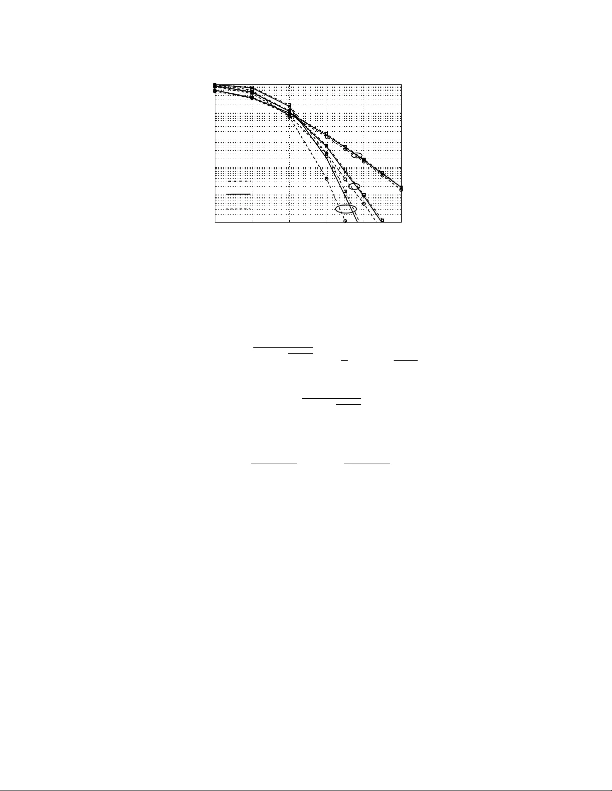
1 Inﬁnity-Norm Sphere-Decoding Dominik Seethaler and Helmut B ¨ olcskei Communication T echnology Laboratory ETH Zurich 8092 Zurich, Switzerland { seethal, boelcskei } @nari.ee.ethz.ch Abstract The most promising approaches for efﬁcient detection in multiple-input multiple-output (MIMO) wireless systems are based on sphere-decoding (SD). The con ventional (and optimum) norm that is used to conduct the tree trav ersal step in SD is the l 2 -norm. It was, howe ver , recently observed that using the l ∞ -norm instead reduces the hardware complexity of SD considerably at only a marginal performance loss. These savings result from a reduction in the length of the critical path in the circuit and the silicon area required for metric computation, but are also, as observed previously through simulation results, a consequence of a reduction in the computational (i.e ., algorithmic) complexity . The aim of this paper is an analytical performance and computational complexity analysis of l ∞ -norm SD. For i.i.d. Rayleigh fading MIMO channels, we show that l ∞ -norm SD achieves full div ersity order with an asymptotic SNR gap, compared to l 2 -norm SD, that increases at most linearly in the number of receive antennas. Moreover , we provide a closed-form expression for the computational complexity of l ∞ -norm SD based on which we establish that its complexity scales exponentially in the system size. Finally , we characterize the tree pruning behavior of l ∞ -norm SD and show that it behav es fundamentally dif ferent from that of l 2 -norm SD. Index T erms MIMO wireless, data detection, sphere-decoding, maximum-likelihood, inﬁnity norm, hardware complexity , algorithmic complexity This work was supported in part by the STREP project No. IST -026905 (MASCOT) within the Sixth Framew ork Programme of the European Commission. P art of this work w as performed while D. Seethaler was with the Institute of Communications and Radio-Frequency Engineering, V ienna Uni versity of T echnology . This paper was presented in part at IEEE ISIT 2008, T oronto, ON, Canada, July 2008. October 22, 2018 DRAFT 2 I . I N T RO D U C T I O N Multiple-input multiple-output (MIMO) wireless systems of fer considerable gains ov er single- antenna systems, in terms of throughput and link reliability , see, e.g., [1]. These gains come, ho wev er , at a signiﬁcant increase in recei ver comple xity . In particular , one of the most challenging problems in MIMO recei ver design is the de velopment of hardware-ef ﬁcient data detection algorithms achie ving (close-to) optimum performance [2]. Among the most promising approaches to the solution of this problem is the so-called sphere-decoding (SD) algorithm [3]–[8], which performs optimum, i.e., maximum-likelihood (ML), detection through a weighted tree search. SD exhibits (often signiﬁcantly) smaller computational complexity than exhausti ve search ML detection [2], [9]. A. Har dwar e Implementation Aspects of SD Hardware implementations of sev eral v ariants of the SD algorithm are described in [2], [7]. It is argued in [7] that the ov erall hardware complexity of a SD is essentially determined by (i) the computational (i.e., algorithmic) complexity in terms of the number of nodes visited in the tree search and (ii) the cir cuit complexity in terms of the length of the critical path in the circuit and the required silicon area for metric computation. The length of the critical path limits the clock frequency of the circuit [10]. One of the main ﬁndings of [7] is that replacing the l 2 -norm in the ML detector by the l ∞ -norm and hence trav ersing the search tree based on the l ∞ -metric incurs only a small performance loss while signiﬁcantly reducing the ov erall hardware complexity of SD by virtue of a reduction of both the computational and the circuit complexity . T o understand where the reduction in circuit comple xity comes from, we refer to Fig. 1 (cf., [7, Fig. 2]) sho wing tradeoff curves between circuit area and the length of the critical path corresponding to the computation of the metrics x 2 1 + x 2 2 (squared l 2 -norm) and max {| x 1 | , | x 2 |} ( l ∞ -norm) for x 1 , x 2 ∈ R . These tradeoffs can be achie ved by choosing dif ferent hardw are implementations of the corresponding metric computation circuit. From Fig. 1 it can be seen that the computation of max {| x 1 | , | x 2 |} can be implemented much more ef ﬁciently in hardware than the computation of x 2 1 + x 2 2 . The main reason for this is that ev aluating max {| x 1 | , | x 2 |} , in contrast to x 2 1 + x 2 2 , does not require squaring operations. Replacing the l 2 - by the l ∞ -norm also has an impact on the computational complexity of SD. In particular , it was observed in [7], through simulation results, that SD based on the l ∞ -norm (referred to as SD- l ∞ ) exhibits lower DRAFT October 22, 2018 D. SEETHALER AND H. B ¨ OLCSKEI: INFINITY -NORM SPHERE-DECODING 3 Area [GE] Critical path length reduction 0 0.5 1 1.5 2 2.5 3 0 500 1000 1500 Critical Path [ns] abs max abs ^2 ^2 + W W 2W W Fig. 1. Circuit area and critical path length tradeoff curves corresponding to the computation of x 2 1 + x 2 2 (squared l 2 -norm) and max {| x 1 | , | x 2 |} ( l ∞ -norm) for x 1 , x 2 ∈ R . The area is giv en in gate-equiv alents (GE) and the length of the critical path is giv en in nano seconds (ns). W denotes the word length. computational complexity than SD based on the l 2 -norm (referred to as SD- l 2 ). Furthermore, the results in [7] indicate that the overall complexity (determined by both the circuit and the computational complexity) of SD- l ∞ is up to a factor of 5 lower than the overall complexity of SD- l 2 . SD- l ∞ therefore appears to be a promising approach to near-optimum MIMO detection at lo w hardware complexity . B. Contrib utions The aim of this paper is to deepen the understanding of SD- l ∞ through an analytical perfor - mance and computational complexity analysis for i.i.d. Rayleigh fading MIMO channels. Our main contributions can be summarized as follows: • W e show that SD- l ∞ achie ves the same (i.e., full) di versity order as SD- l 2 . • W e show that the gap in signal-to-noise ratio (SNR) incurred by SD- l ∞ , compared to SD- l 2 , increases at most linearly in the number of recei ve antennas. • W e deriv e a closed-form expression for the complexity of SD- l ∞ . Here and in the remainder of the paper , complexity is deﬁned as the average number of nodes visited in the tree search, where av eraging is performed with respect to the (random) channel, noise, and transmit signal. Corresponding results for SD- l 2 can be found in [9], [11]–[13]. • W e prove that the complexity of SD- l ∞ scales e xponentially in the number of transmit antennas. Our proof technique directly extends to SD- l 2 and thus yields an alternativ e (vis- ` a-vis [14]) proof of the exponential complexity scaling behavior of SD- l 2 . October 22, 2018 DRAFT 4 • Finally , we provide insights into the tree pruning beha vior of SD- l ∞ relati ve to that of SD- l 2 . In particular , based on an asymptotic (in SNR) analysis of our closed-form comple xity expressions, we show that SD- l ∞ tends to prune more aggressi vely than SD- l 2 at tree lev els closer to the root of the search tree, whereas this behavior is re versed at tree lev els closer to the leav es. C. Outline The paper is organized as follows. After introducing the system model and brieﬂy re vie wing rele vant aspects of SD- l 2 and SD- l ∞ in the remainder of Section I, we analyze the error probability beha vior of SD- l ∞ in terms of div ersity order and SNR gap in Section II. In Section III, we deri ve a closed-form e xpression for the complexity of SD- l ∞ . This result is then used to establish the e xponential complexity scaling beha vior (in the number of transmit antennas) of SD- l ∞ and to analyze, in Section IV, the tree pruning behavior of SD- l ∞ by means of an asymptotic (in SNR) analysis. In Section V, we report modiﬁcations of the results presented in Section II and Section III to account for the slightly modiﬁed metric used in the hardware implementations reported in [7]. Numerical results are provided in Section VI. Section VII concludes the paper . D. Notation W e write A i,j for the entry in the i th row and j th column of the matrix A and x i for the i th entry of the vector x . For unitary A , we hav e A H A = AA H = I , where H denotes conjugate transposition, i.e., transposition T follo wed by element-wise comple x conjugation ∗ , and I is the identity matrix. The l 2 - and the l ∞ -norm of a vector x = ( x 1 · · · x M ) T ∈ C M are deﬁned as k x k 2 = p | x 1 | 2 + · · · + | x M | 2 and k x k ∞ = max  | x 1 | , . . . , | x M |  , respecti vely . W e will also need the l f ∞ -norm k x k f ∞ = max  | x R , 1 | , | x I , 1 | , . . . , | x I ,M |  , where x R and x I denote the real and imaginary parts, respecti vely , of x ∈ C . W e note that the l 2 -norm is in variant with respect to (w .r .t.) unitary transformations, i.e., k x k 2 = k Ax k 2 if A is unitary . E {·} stands for the expectation operator and Φ x ( s ) = E { e sx } refers to the moment generating function (MGF) of the random v ariable (R V) x . W e write x ∼ χ a if the R V x is χ -distributed with a ≥ 0 degrees of freedom and normalized such that E { x 2 } = a . The probability density function (pdf) of the R V x ∼ χ a is then gi ven by [15] f x ( t ) = 2 1 − a/ 2 Γ( a/ 2) t a − 1 e − t 2 2 , t ≥ 0 (1) DRAFT October 22, 2018 D. SEETHALER AND H. B ¨ OLCSKEI: INFINITY -NORM SPHERE-DECODING 5 and f x ( t ) = 0 , t < 0 , where Γ( a ) = R ∞ 0 y a − 1 e − y dy refers to the Gamma function. For the corresponding cumulati ve distribution function (cdf) we have P  x ≤ t  = γ a/ 2 ( t 2 / 2) . Here, γ a ( t ) denotes the (regularized) lower incomplete Gamma function; some important properties of γ a ( t ) are stated in Appendix C. W e denote a circularly symmetric complex Gaussian R V with v ariance σ 2 x as x ∼ C N (0 , σ 2 x ) ; x ∼ N ( µ x , σ 2 x ) refers to a real-valued Gaussian distributed R V x with mean µ x and variance σ 2 x . For independently and identically distrib uted (i.i.d.) R Vs x i ∼ N (0 , 1) , i = 1 , . . . , a , we have z = p x 2 1 + · · · + x 2 a ∼ χ a . Furthermore, if the R V x is χ a - distributed, x 2 is χ 2 a -distributed. W e write y ∼ χ 2 a if the R V y is χ 2 a -distributed with E { y } = a . In particular , the MGF of the R V y ∼ χ 2 a is gi ven by Φ y ( s ) = (1 − 2 s ) − a/ 2 (2) for any s < 1 / 2 . The Q-function is deﬁned as Q ( x ) =  1 / √ 2 π  R ∞ x e − y 2 / 2 dy , for x ≥ 0 . For equality in distribution we write d = . Furthermore, the “Big O” notation g ( x ) = O ( f ( x )) , x → x 0 , denotes that | g ( x ) /f ( x ) | remains bounded as x → x 0 [16]. The “little o” notation g ( x ) = o ( f ( x )) , x → x 0 , stands for lim x → x 0 g ( x ) /f ( x ) = 0 , and g ( x ) a ∼ f ( x ) , x → x 0 , means that lim x → x 0 g ( x ) /f ( x ) = 1 . By g ( x )  f ( x ) , x → x 0 , and g ( x )  f ( x ) , x → x 0 , for positi ve functions g ( x ) and f ( x ) , we denote lim x → x 0 g ( x ) /f ( x ) ≤ 1 and lim x → x 0 g ( x ) /f ( x ) > 1 , respecti vely . The Dirac delta function is referred to as δ ( x ) , con volution is denoted as ∗ , and the natural logarithm to the base e is referred to as log ( · ) . The summations in P x and P x 6 = x 0 are ov er all possible values of x and ov er all possible values of x except for x 0 , respectiv ely . Finally , f ( n ) ( x ) refers to the n th deri vati v e of the function f ( x ) and f 0 ( x ) = f (1) ( x ) . E. System Model W e consider an N × M MIMO system with M transmit antennas and N ≥ M receiv e antennas. The corresponding complex-baseband input-output relation is giv en by r = Hd 0 + w where d 0 = ( d 0 1 · · · d 0 M ) T denotes the transmitted data v ector , H is the N × M channel matrix, r = ( r 1 · · · r N ) T is the receiv ed vector , and w = ( w 1 · · · w N ) T denotes the additiv e noise vector . The symbols d 0 m , drawn from a ﬁnite alphabet A , hav e zero-mean and unit variance. Furthermore, we assume that the H n,m are i.i.d. C N (0 , 1 / M ) and the w n are i.i.d. C N (0 , σ 2 ) . The SNR (per recei ve antenna) is therefore gi ven by ρ = 1 /σ 2 . October 22, 2018 DRAFT 6 F . Spher e-Decoding W e no w brieﬂy revie w SD based on the l 2 -norm [3]–[6], [8] and (suboptimum) SD based on the l ∞ -norm [7]. 1) SD based on the l 2 -norm: SD- l 2 performs ML detection by ﬁnding b d ML = arg min d ∈A M k r − Hd k 2 2 (3) through a tree search subject to a sphere constraint (SC), which amounts to considering only those data vectors d that satisfy k r − Hd k 2 2 ≤ C 2 2 (kno wn as the Fincke-Pohst [3] strategy). Here, the radius C 2 has to be chosen sufﬁciently lar ge for the corresponding search sphere to contain at least one data vector . Note, howe ver , that if C 2 is chosen too large, too man y points will satisfy the SC and the complexity of SD- l 2 will be high (for guidelines on how to choose C 2 see [9], [17] and Section III-E). The SC is then cast into a weighted tree search problem by ﬁrst performing a QR-decomposition of H resulting in H = Q h R 0 i where Q is an N × N unitary matrix, R is an M × M upper triangular matrix, and 0 denotes an all-zeros matrix of size ( N − M ) × M . Then, the SC can equiv alently be written as k z ( d ) k 2 2 ≤ C 2 2 (4) where z ( d ) = y − h R 0 i d with y = Q H r = h R 0 i d 0 + n . (5) Here, the unitarity of Q implies that n = Q H w is again i.i.d. C N (0 , σ 2 ) . The data subv ectors d k ∈ A k of length k d k = ( d M − k +1 · · · d M ) T , k = 1 , . . . , M , can be arranged in a tree with root abo ve le vel k = 1 and corresponding leav es at lev el k = M ; a speciﬁc d k is associated with a node in this tree at le vel k . Let us deﬁne z k ( d k ) = y k − h R k 0 i d k as the vector containing the bottom k + L with L = N − M elements of z ( d ) in (5). Here, R k denotes the k × k upper triangular submatrix of R associated with d k and DRAFT October 22, 2018 D. SEETHALER AND H. B ¨ OLCSKEI: INFINITY -NORM SPHERE-DECODING 7 y k = ( y M − k +1 · · · y M y M +1 · · · y N ) T . The metric k z ( d ) k 2 2 = k z M ( d M ) k 2 2 can then be computed recursi vely according to k z k ( d k ) k 2 2 = k z k − 1 ( d k − 1 ) k 2 2 +   [ z ( d )] M − k +1   2 , k = 1 , . . . , M , (6) where   [ z ( d )] M − k +1   2 =      y M − k +1 − M X i = M − k +1 R M − k +1 ,i d i      2 . (7) Thus, with (6), a necessary condition for d to satisfy the SC (4) is that any associated d k satisﬁes the partial SC (PSC) k z k ( d k ) k 2 2 ≤ C 2 2 . (8) Consequently , we can ﬁnd all data vectors inside the search sphere, i.e., all data vectors satisfying the SC (4), through a weighted tree search. The tree is trav ersed starting at lev el k = 1 . If the PSC is violated by a giv en d k , the node associated with that d k along with all its children is pruned from the tree. The ML solution (3) is found by choosing, among all surviving leaf nodes d = d M , the one with minimum k z ( d ) k 2 . 2) SD based on the l ∞ -norm: W e deﬁne SD- l ∞ as the algorithm obtained by replacing the SC (4) by the box constr aint (BC) k z ( d ) k ∞ ≤ C ∞ . The metric k z ( d ) k ∞ can be computed recursi vely according to k z k ( d k ) k ∞ = max  k z k − 1 ( d k − 1 ) k ∞ ,   [ z ( d )] M − k +1    . Consequently , the PSC is replaced by the partial box constraint (PBC) k z k ( d k ) k ∞ ≤ C ∞ . (9) If the PBC is violated by a gi ven d k , the node associated with that d k along with all its children is pruned from the tree. The l ∞ -optimal solution is obtained by choosing, among all surviving leaf nodes d = d M , the one with minimum k z ( d ) k ∞ , i.e., b d ∞ = arg min d ∈A M k z ( d ) k ∞ . (10) Slightly ab using terminology , we call the side length C ∞ of the search box the “ radius ” associated with SD- l ∞ . Like in the SD- l 2 case with C 2 , here the radius C ∞ has to be chosen lar ge enough to ensure that at least one data vector is found by the algorithm. Again, ho wev er , choosing C ∞ too large will in general result in a high complexity of SD- l ∞ (for guidelines on how to choose C ∞ we refer to Section III-E). October 22, 2018 DRAFT 8 W e emphasize the following aspects of SD- l ∞ : • The SD- l ∞ hardware implementation reported in [7] is actually based on the l f ∞ - norm k x k f ∞ = max  | x R , 1 | , | x I , 1 | , . . . , | x I ,M |  rather than the l ∞ -norm k x k ∞ = max  | x 1 | , . . . , | x M |  , x ∈ C M . Here, the essential aspect is that the computation of the l f ∞ -norm, as opposed to the l ∞ - and the l 2 -norm, does not require squaring operations, which, as already noted in Section I-A, results in signiﬁcantly smaller circuit comple xity . Ne vertheless, in the follo wing, for the sake of simplicity of exposition, we ﬁrst analyze SD- l ∞ , i.e., SD based on the con ventional l ∞ -norm, thereby re vealing the fundamental aspects (w .r .t. performance and complexity) of SD using the l f ∞ -norm (referred to as SD- l f ∞ ). The modiﬁcations of the results on SD- l ∞ needed to account for the use of the l f ∞ -norm are described in Section V. • The tree search strategy underlying SD- l ∞ is identical to that of Kannan’ s strate gy (see, e.g., [5], [18]), which also ﬁnds all data vectors inside a hypercube. The dif ference between SD- l ∞ and Kannan’ s algorithm lies in calculating the ﬁnal detection result. SD- l ∞ implements (10) while Kannan’ s approach is optimum as it implements (3). Optimality of Kannan’ s algorithm is achie ved through (i) guaranteeing that the solution of (3) is contained inside the search hypercube (which, in general, necessitates choosing the search radius to be larger than the corresponding radius for SD- l ∞ and hence incurs a higher complexity) and (ii) in the last step comparing all found data vectors with respect to their l 2 -distance k r − Hd k 2 (which, in contrast to SD- l f ∞ , necessitates squaring operations). • Finally , we emphasize that SD- l ∞ as deﬁned abov e does not correspond to l ∞ -norm decoding on the “full” channel matrix H according to b d ∞ , full = arg min d ∈A M k r − Hd k ∞ (11) since k r − Hd k ∞ 6 = k z ( d ) k ∞ , in general. This statement also holds true for SD based on the l f ∞ -norm. In the l 2 -norm case detection on the full channel matrix H is equiv alent to detection on the upper triangular matrix R . I I . E R RO R P R O B A B I L I T Y O F S D - l ∞ In this section, we show that SD- l ∞ achie ves the same div ersity order as ML (i.e., SD- l 2 ) detection and we quantify the SNR loss incurred by SD- l ∞ . DRAFT October 22, 2018 D. SEETHALER AND H. B ¨ OLCSKEI: INFINITY -NORM SPHERE-DECODING 9 A. Distance Pr operties W e start by in vestigating distance properties of the SD- l ∞ solution b d ∞ . Using the bounds 1 N k x k 2 2 ≤ k x k 2 ∞ ≤ k x k 2 2 , (12) v alid for any vector x ∈ C N , we obtain   r − H b d ∞   2 2 =    y − h R 0 i b d ∞    2 2 ≤ N    y − h R 0 i b d ∞    2 ∞ ≤ N    y − h R 0 i b d ML    2 ∞ ≤ N    y − h R 0 i b d ML    2 2 = N   r − H b d ML   2 2 . (13) W e are therefore guaranteed that   r − H b d ∞   2 lies within a factor of √ N of the minimum distance   r − H b d ML   2 realized by the ML detector (3). Tri vially , SD- l ∞ is optimum for N = 1 (simply because the l ∞ -norm equals the l 2 -norm in this case). For increasing N , (13) suggests an increasing performance loss incurred by SD- l ∞ when compared to the ML detector (i.e., SD- l 2 ). In the next section, we quantify this performance loss in terms of div ersity order and SNR gap. W e note that for Babai’ s nearest plane algorithm [19] (which can be interpreted as a decision-feedback detector in combination with LLL lattice reduction, see, e.g., [5]), we get a result that is structurally similar to (13) when b d ∞ is replaced by Babai’ s detection result and the factor N is replaced by 2 ( N − 1) . Consequently , the performance loss incurred by Babai’ s nearest plane algorithm can be expected to be signiﬁcantly larger than that incurred by SD- l ∞ . B. Diversity Order and SNR Gap W e denote the error probability as a function of SNR ρ as P ( ρ ) . In the following, we will only encounter error probabilities of the form P ( ρ ) = ( K ρ ) − δ + o ( ρ − δ ) , ρ → ∞ , with some constant K > 0 not depending on ρ . W e can deﬁne the corresponding SNR exponent δ as [20], [21] δ = − lim ρ → ∞ log P ( ρ ) log ρ . (14) Furthermore, if P 1 ( ρ ) and P 2 ( ρ ) hav e the same SNR exponent, we can deﬁne an asymptotic SNR gap α via P 1 ( ρ ) a ∼ P 2 ( α ρ ) , ρ → ∞ . For example, if P 1 ( ρ ) = ( K 1 ρ ) − δ + o ( ρ − δ ) and P 2 ( ρ ) = ( K 2 ρ ) − δ + o ( ρ − δ ) , we ha ve α = K 1 /K 2 . Our analysis corresponds to multiplexing gain r = 0 in the frame work of [21]. The corresponding results bear practical signiﬁcance as it can be October 22, 2018 DRAFT 10 sho wn, for example, that ev en for r = 0 con ventional suboptimum detection schemes like linear equalization-based or V -BLAST detectors are unable to achiev e the full div ersity order of N [1], [21], [22]. In the following, we ﬁrst focus on the beha vior of the pairwise error probability (PEP) and then analyze the total error probability . 1) P airwise Err or Pr obability: Assume that the data vector d 0 was transmitted. The probability of erroneously deciding in fav or of another data vector d 6 = d 0 is denoted as P d 0 → d , ML ( ρ ) in the SD- l 2 case and P d 0 → d , ∞ ( ρ ) in the SD- l ∞ case. T o deri ve (an upper bound on) P d 0 → d , ∞ ( ρ ) , we ﬁrst present a somewhat uncon ventional approach for upper -bounding P d 0 → d , ML ( ρ ) , which lends itself nicely to an extension to the l ∞ -case. W e start from P d 0 → d , ML ( ρ ) = P h k r − Hd k 2 ≤ k r − Hd 0 k 2 i = P h k Hb + w k 2 ≤ k w k 2 i with the error (difference) vector b = d 0 − d . Applying the in v erse triangle inequality according to k Hb + w k 2 ≥   k Hb k 2 − k w k 2   , we further obtain P d 0 → d , ML ( ρ ) ≤ P  k w k 2 ≥ 1 2 k Hb k 2  (15) noting that | x | ≥ x , for all x ∈ R . W ith √ 2 σ k w k 2 ∼ χ 2 N , conditioning on H , and applying the Chernof f upper bound yields P  k w k 2 ≥ 1 2 k Hb k 2    H  ≤ Φ χ 2 2 N ( s ) e − sρ k Hb k 2 2 2 for s ∈ [0 , 1 / 2) . Here, Φ χ 2 2 N ( s ) denotes the MGF of a χ 2 2 N -distributed R V (see (2)). A veraging ov er H then results in P d 0 → d , ML ( ρ ) ≤ Φ χ 2 2 N ( s ) E H  e − sρ k Hb k 2 2 2  = Φ χ 2 2 N ( s )  1 + sρ k b k 2 2 2 M  − N (16) because 2 M k Hb k 2 2 / k b k 2 2 ∼ χ 2 2 N for a gi ven b . For high SNR, the right hand side (RHS) of (16) is minimized for s = 1 / 4 , which giv es P d 0 → d , ML ( ρ ) ≤ 2 N  1 + ρ k b k 2 2 8 M  − N . (17) Since N is the maximum di versity order that can be achie ved o ver an N × M MIMO channel with the transmission setup considered in this paper (i.e., spatial multiplexing) [21], we can DRAFT October 22, 2018 D. SEETHALER AND H. B ¨ OLCSKEI: INFINITY -NORM SPHERE-DECODING 11 immediately conclude that the SNR exponent of P d 0 → d , ML ( ρ ) equals N for any non-zero b (see also the lo wer bound (22) on P d 0 → d , ML ( ρ ) having an SNR exponent of N as well). For SD- l ∞ we can follo w a similar approach. Starting with (10), we get P d 0 → d , ∞ ( ρ ) ≤ P h k z ( d ) k ∞ ≤ k z ( d 0 ) k ∞ i = P     h R 0 i b + n    ∞ ≤ k n k ∞  . (18) Note that for SD- l ∞ , unlike for SD- l 2 , the ev ent k z ( d ) k ∞ = k z ( d 0 ) k ∞ can, in general, occur with non-zero probability . Declaring an error in this case certainly yields an upper bound on P d 0 → d , ∞ ( ρ ) . Next, we apply the upper and lower bounds in (12) and exploit the in v ariance of the l 2 -norm to unitary transformations to get P d 0 → d , ∞ ( ρ ) ≤ P  1 √ N    h R 0 i b + n    2 ≤ k n k 2  = P  1 √ N k Hb + w k 2 ≤ k w k 2  . (19) Finally , applying the in v erse triangle inequality according to k Hb + w k 2 ≥   k Hb k 2 − k w k 2   , we hav e P d 0 → d , ∞ ( ρ ) ≤ P  k w k 2 ≥ 1 √ N + 1 k Hb k 2  . (20) Note the structural similarity of (20) and (15). Emplo ying the same ar guments as in the SD- l 2 case, we get P  k w k 2 ≥ 1 √ N + 1 k Hb k 2    H  ≤ Φ χ 2 2 N ( s ) e − sρ 2 k Hb k 2 2 ( √ N + 1) 2 for s ∈ [0 , 1 / 2) . A veraging ov er H then results in P d 0 → d , ∞ ( ρ ) ≤ 2 N  1 + ρ k b k 2 2 2  √ N + 1  2 M  − N = UB ∞ ( ρ ) (21) where we used the fact that s = 1 / 4 minimizes the upper bound for high SNR. As in the SD- l 2 case for P d 0 → d , ML ( ρ ) , we can immediately conclude that the SNR exponent of P d 0 → d , ∞ ( ρ ) equals N for any non-zero b . There is, howe ver , an SNR gap between P d 0 → d , ∞ ( ρ ) and P d 0 → d , ML ( ρ ) , which can be quantiﬁed as follo ws. W e start by e valuating [23, Eq. (20)] for the case at hand to get P d 0 → d , ML ( ρ ) ≥ 1 2 1 4 N  2 N N   1 + ρ k b k 2 2 4 M  − N = LB ML ( ρ ) . (22) October 22, 2018 DRAFT 12 The asymptotic SNR gap between UB ∞ ( ρ ) and LB ML ( ρ ) , denoted as β , i.e., UB ∞ ( ρ ) a ∼ LB ML ( ρ/β ) , ρ → ∞ , is directly obtained as β = 4  √ N + 1  2  1 2  2 N N  − 1 N . (23) W e can thus conclude that the asymptotic SNR gap between the PEP for SD- l ∞ and the PEP for SD- l 2 is upper-bounded by β , or , equiv alently , we hav e P d 0 → d , ∞ ( ρ )  P d 0 → d , ML ( ρ/β ) , ρ → ∞ . (24) 2) T otal Err or Pr obability: In the following, we consider the total error probability P E ( ρ ) = P  d 0 6 = b d  assuming equally likely transmitted data vectors d 0 . If not speciﬁed, P E ( ρ ) stands for the total error probability P E ∞ ( ρ ) of SD- l ∞ and P E ML ( ρ ) of SD- l 2 . W e start by noting that P E ( ρ ) = |A| − M X d 0 P E | d 0 ( ρ ) . (25) Here, P E | d 0 ( ρ ) refers to the total error probability conditioned on d 0 being transmitted, which can be bounded as P d 0 → any d ( ρ ) ≤ P E | d 0 ( ρ ) ≤ X d 6 = d 0 P d 0 → d ( ρ ) . (26) It follo ws that P E ( ρ ) ≤ |A| − M X d 0 X d 6 = d 0 P d 0 → d ( ρ ) (27) and P E ( ρ ) ≥ |A| − M X d 0 P d 0 → any d ( ρ ) . (28) As the SNR exponent of P d 0 → d , ∞ ( ρ ) equals N for all b = d − d 0 6 = 0 (cf. (21)), we can conclude that SD- l ∞ achie ves full diversity or der N and hence the same diversity order as ML detection. The corresponding asymptotic SNR gap is obtained as follo ws. W ith (24)-(27), we get P E ∞ ( ρ )  |A| − M X d 0 X d 6 = d 0 P d 0 → d , ∞ ( ρ ) , ρ → ∞  |A| − M X d 0 X d 6 = d 0 P d 0 → d , ML ( ρ/β ) , ρ → ∞  |A| − M X d 0 X d 6 = d 0 P E ML | d 0 ( ρ/β ) , ρ → ∞  |A| M P E ML ( ρ/β ) , ρ → ∞ . (29) DRAFT October 22, 2018 D. SEETHALER AND H. B ¨ OLCSKEI: INFINITY -NORM SPHERE-DECODING 13 From (27) together with (17) and (28) together with (22), we can conclude that P E ML ( ρ ) has SNR exponent N and can be written as P E ML ( ρ ) = ( K ML ρ ) − N + o ( ρ − N ) , ρ → ∞ , with some constant K ML > 0 that does not depend on ρ . W ith P E ∞ ( ρ )  |A| M P E ML ( ρ/β ) from (29) and N ≥ M , this yields P E ∞ ( ρ )  P E ML  ρ/ ( |A| β )  , which establishes that the asymptotic SNR gap incurred by SD- l ∞ is upper-bounded by |A| β with β speciﬁed in (23). Furthermore, using  m l  ≥  m l  l , we hav e  2 N N  ≥ 2 N , which, when employed in (23), sho ws that β ≤ 4  √ N +1  2 ≤ 16 N . Thus, the asymptotic SNR gap between the total error probabilities P E ML ( ρ ) and P E ∞ ( ρ ) is upper-bounded by 16 |A| N . W e can therefore conclude that the asymptotic SNR gap incurred by SD- l ∞ scales at most linearly in the number of receiv e antennas. Simulation results (see Section VI-A) rev eal that the actual SNR gap is much smaller than 16 |A| N . W e ﬁnally note that applying [24, Prop. 1] shows that the statement on SD- l ∞ achie ving full di versity order for the i.i.d. Rayleigh fading case directly extends to more general fading statistics such as spatially correlated Rayleigh or Ricean fading. 3) l ∞ -Norm Decoding on Full Channel Matrix: As pointed out in Section I-F2, SD- l ∞ does not correspond to l ∞ -norm decoding on the full channel matrix H according to (11). Ho wev er , as the PEP of l ∞ -norm decoding on the full channel matrix satisﬁes P d 0 → d , ∞ , H ( ρ ) = P h k Hb + w k ∞ ≤ k w k ∞ i , we can apply the upper and lo wer bounds in (12) to arriv e at P d 0 → d , ∞ , H ( ρ ) ≤ P  1 √ N k Hb + w k 2 ≤ k w k 2  which is exactly the same upper bound as that obtained for SD- l ∞ in (19). W e can therefore conclude that l ∞ -norm decoding on the full channel matrix H also achiev es full div ersity order with an asymptotic SNR gap, vis- ` a-vis SD- l 2 , that increases at most linearly in the number of recei ve antennas. I I I . C O M P L E X I T Y O F S D - l ∞ In this section, we analyze the complexity of SD- l ∞ by deriving an analytic expression for the av erage number of nodes visited in the tree search when pruning according to the PBC (9) is performed. A node d k is visited if and only if its corresponding PBC (9) is satisﬁed. W e consider a ﬁx ed choice of C ∞ and av erage w .r .t. channel, noise, and transmit signal. Based on October 22, 2018 DRAFT 14 the analytic complexity expression for SD- l ∞ , it is then shown that the complexity of SD- l ∞ scales exponentially in the number of transmit antennas M . A. Basic Appr oac h Our methodology is similar to that adopted in [9] for SD- l 2 . The key dif ference to the approach in [9] lies in the computation of the partial metric cdfs as detailed in Section III-B. For a gi ven C ∞ , a simple counting argument yields the number of nodes S ∞ ,k visited at tree le vel k , k = 1 , . . . , M , as S ∞ ,k = X d k I ( z k ( d k )) (30) where I ( z k ( d k )) =      1 , if k z k ( d k ) k ∞ ≤ C ∞ 0 , otherwise . W e trivially hav e S ∞ ,k ≤ |A| k . First, we note that E { I ( z k ( d k )) } = P  k z k ( d k ) k ∞ ≤ C ∞  , where the expectation is w .r .t. the channel R , noise n , and data vector d 0 . Consequently , we hav e E { S ∞ ,k } = X d k P  k z k ( d k ) k ∞ ≤ C ∞  (31) with the total complexity E { S ∞ } = M X k =1 E { S ∞ ,k } . (32) Next, we condition on the data subv ector d 0 k ∈ A k and write P  k z k ( d k ) k ∞ ≤ C ∞ | d 0 k  = P  k z k ( b k ) k ∞ ≤ C ∞  with z k ( b k ) = h R k 0 i b k + h n k n L i (33) where b k = d 0 k − d k is a pairwise error subv ector , n k = ( n M − k +1 · · · n M ) T , and n L = ( n M +1 · · · n N ) T . W e set z ( b ) = z M ( b M ) and note that z k ( b k ) =  [ z ( b )] M − k +1 · · · [ z ( b )] N  T . Formally , for a giv en d 0 k , we will often speak of “a node” b k , which, in a one-to-one fashion, refers to the node d k = d 0 k − b k in the search tree. For example, the node d k = d 0 k corresponding to the transmitted data subvector d 0 k is equiv alent to node b k = 0 . If we speak of a node b k DRAFT October 22, 2018 D. SEETHALER AND H. B ¨ OLCSKEI: INFINITY -NORM SPHERE-DECODING 15 without specifying d 0 k , the corresponding statements hold for all pairs d 0 k , d k ∈ A k satisfying b k = d 0 k − d k . It follo ws that (31) can be written as E { S ∞ ,k } = 1 |A| k X d k X d 0 k P  k z k ( d k ) k ∞ ≤ C ∞ | d 0 k  = 1 |A| k X b k P  k z k ( b k ) k ∞ ≤ C ∞  (34) where we assumed equally likely transmitted data subvectors d 0 k for all tree lev els k = 1 , . . . , M ; this holds, e.g., for statistically independent (across the transmit antennas) and equally likely data symbols. The sum in (34) is taken over all possible combinations of pairwise error sub vectors b k . Equi valently , the complexity at the k th tree le vel E { S 2 ,k } for SD- l 2 is giv en by (34) with the l ∞ -norm replaced by the l 2 -norm and C ∞ replaced by C 2 , i.e., E { S 2 ,k } = 1 |A| k X b k P  k z k ( b k ) k 2 ≤ C 2  . (35) W e ﬁnally note that P  k z k ( b k ) k ∞ ≤ C ∞  in (34) and P  k z k ( b k ) k 2 ≤ C 2  in (35) express the probability that node b k is visited by SD- l ∞ and SD- l 2 , respectiv ely , and are equi v alent to the av erage (w .r .t. the channel R and noise n ) number of visits of node b k by SD- l ∞ and SD- l 2 , respecti vely . B. Computation of the P artial Metric Cdfs From (34) and (35) we can see that the computation of E { S ∞ ,k } and E { S 2 ,k } requires kno wledge of the cdfs of the partial metrics k z k ( b k ) k ∞ and k z k ( b k ) k 2 , respecti vely (recall that the radii C ∞ and C 2 are assumed to be ﬁx ed and independent of the channel, noise, and data realizations). An analytic expression for P  k z k ( b k ) k 2 ≤ C 2  was provided in [9], [11]. More speciﬁcally , it is sho wn in [9, Lemma 1] that thanks to the in v ariance of the l 2 -norm w .r .t. unitary transformations k z k ( b k ) k 2 d =    H k b k + h n k n L i    2 where the ( k + L ) × k matrix H k with L = N − M has i.i.d. C N (0 , 1 / M ) entries. Conditioned on b k , the R V    H k b k + h n k n L i    2 is then easily found to be χ k + L -distributed, which leads to an expression for P  k z k ( b k ) k 2 ≤ C 2  in terms of the lower incomplete Gamma function (see also October 22, 2018 DRAFT 16 Section III-C). As the l ∞ -norm is not in v ariant w .r .t. unitary transformations, this approach does not carry over to the l ∞ -case considered here. Instead, we follow a direct approach as detailed belo w . 1) Cdf of k z k ( b k ) k ∞ : Since the nonzero entries in R are statistically independent [25, Lemma 2.1], the elements of z k ( b k ) conditioned on b k are statistically independent as well. W e thus hav e P  k z k ( b k ) k ∞ ≤ C ∞  = k + L Y i =1 P h   [ z k ( b k )] i   ≤ C ∞ i . (36) The bottom L elements of z k ( b k ) are gi ven by the i.i.d. C N (0 , σ 2 ) vector n L (see (33)) so that P h   [ z k ( b k )] i   ≤ C ∞ i = γ 1  C 2 ∞ σ 2  , i = k + 1 , . . . , k + L, which yields P  k z k ( b k ) k ∞ ≤ C ∞  =  γ 1  C 2 ∞ σ 2  L k Y m =1 P h   [ z ( b )] M − m +1   ≤ C ∞ i . (37) 2) Cdf of   [ z ( b )] M − m +1   : An analytic expression for P h   [ z ( b )] M − m +1   ≤ C ∞ i can be obtained via direct integration using the f act that the nonzero entries of R are statistically independent with √ 2 M R i,i ∼ χ 2( N − i +1) and R i,j ∼ C N (0 , 1 / M ) , for i = 1 , . . . , M , j > i [25, Lemma 2.1]. In Appendix A it is sho wn that P h   [ z ( b )] M − m +1   ≤ C ∞ i is a binomial mixture of χ -distributions with degrees of freedom reaching from 2 up to 2( m + L ) . More speciﬁcally , for m = 1 , . . . , M , we ha ve P h   [ z ( b )] M − m +1   ≤ C ∞ i = m + L − 1 X l =0 B l ( b m ) γ m + L − l  C 2 ∞ k b m k 2 2 / M + σ 2  (38) with the coef ﬁcients B l ( b m ) gi ven by the binomial probabilities B l ( b m ) =  m + L − 1 l  ( p ( b m )) l (1 − p ( b m )) m + L − 1 − l (39) with parameter p ( b m ) = k b m − 1 k 2 2 + M σ 2 k b m k 2 2 + M σ 2 (40) DRAFT October 22, 2018 D. SEETHALER AND H. B ¨ OLCSKEI: INFINITY -NORM SPHERE-DECODING 17 and k b 0 k 2 2 = 0 . In [13] the pdf of the R V   [ z ( b )] M − m +1   2 associated with the distrib ution (38) was obtained in a different form (i.e., not in terms of a binomial mixture of χ -distributions) using an alternativ e deriv ation. More speciﬁcally , the deri v ation in [13] exploits the property k z m ( b m ) k 2 2 = k z m − 1 ( b m − 1 ) k 2 2 +   [ z ( b )] M − m +1   2 with k z m − 1 ( b m − 1 ) k 2 2 and   [ z ( b )] M − m +1   2 being statistically independent and the MGFs of k z m ( b m ) k 2 2 and k z m − 1 ( b m − 1 ) k 2 2 being kno wn from [9]. This allows to compute the MGF of   [ z ( b )] M − m +1   2 and, via the in verse F ourier transform, the corresponding pdf, which can then be used to establish (38). Finally , we note that the direct integration approach used in this paper to obtain (38) can, in contrast to the approach employed in [13], be applied to deri ve the distrib utions of | [ z ( b )] R ,M − m +1 | and | [ z ( b )] I ,M − m +1 | , which are needed to compute (bounds on) the complexity of SD- l f ∞ (see Section V -B for more details). 3) Sum Repr esentation and Moment Generating Function: The binomial mixture representa- tion (38) allows for an interesting alternativ e representation of the R V   [ z ( b )] M − m +1   2 as the sum of independent R Vs. In particular , using results from [26], it is shown in Appendix B that   [ z ( b )] M − m +1   2 d = t 2 m (41) where t 2 m = k b m k 2 2 / M + σ 2 2 γ 2 + m + L − 1 X i =1 λ 2 i ! (42) with the independent R Vs γ 2 and λ 2 i , i = 1 , . . . , m + L − 1 . Here, γ 2 ∼ χ 2 2 with pdf f χ 2 2 ( x ) and the λ 2 i hav e the mixture pdf f λ 2 i ( x ) = (1 − p ( b m )) f χ 2 2 ( x ) + p ( b m ) δ ( x ) (43) or , equiv alently , with probability p ( b m ) the λ 2 i come from a population having pdf δ ( x ) (i.e., they are zero with probability p ( b m ) ) and with probability 1 − p ( b m ) they come from a population having a χ 2 2 distribution. Besides being interesting in its o wn right, the representation (42) allo ws to compute the MGF of   [ z ( b )] M − m +1   2 or , equiv alently , of t 2 m in a straightforward manner , by using (40) and (43), as (cf. (2)) Φ t 2 m ( s ) = E  e st 2 k  = 1 1 − ( k b m k 2 2 / M + σ 2 ) s  1 − p ( b m ) 1 − ( k b m k 2 2 / M + σ 2 ) s + p ( b m )  m + L − 1 = [1 − ( k b m − 1 k 2 2 / M + σ 2 ) s ] m + L − 1 [1 − ( k b m k 2 2 / M + σ 2 ) s ] m + L . (44) October 22, 2018 DRAFT 18 C. Cdf of k z k ( b k ) k 2 Using the results of Section III-B, we can directly recov er the cdf of k z k ( b k ) k 2 obtained in [9]. The deriv ation in [9] is explicitl y based on the rotational in v ariance of the l 2 -norm (see [9, Lemma 1]). Here, we follo w an alternativ e approach and start by using (33) to obtain k z k ( b k ) k 2 2 = k n L k 2 2 + k X m =1   [ z ( b )] M − m +1   2 . Thanks to (41) we then hav e k z k ( b k ) k 2 2 d = k n L k 2 2 + k X m =1 t 2 m . Since the R Vs k n L k 2 2 and t 2 m , m = 1 , . . . , k , are mutually statistically independent, the MGF of k z k ( b k ) k 2 2 can be written as Φ k z k ( b k ) k 2 2 ( s ) = Φ k n L k 2 2 ( s ) k Y m =1 Φ t 2 m ( s ) (45) where Φ k n L k 2 2 ( s ) denotes the MGF of k n L k 2 2 gi ven by (cf. (2)) Φ k n L k 2 2 ( s ) = 1 (1 − σ 2 s ) L . (46) Inserting (44) and (46) into (45), then yields Φ k z k ( b k ) k 2 2 ( s ) = 1 (1 − σ 2 s ) L k Y m =1 [1 − ( k b m − 1 k 2 2 / M + σ 2 ) s ] m + L − 1 [1 − ( k b m k 2 2 / M + σ 2 ) s ] m + L = 1 [1 − ( k b k k 2 2 / M + σ 2 ) s ] k + L which is the MGF of a χ 2 2( k + L ) -distributed R V . Consequently , the cdf of k z k ( b k ) k 2 is gi ven by P  k z k ( b k ) k 2 ≤ C 2  = γ k + L  C 2 2 k b k k 2 2 / M + σ 2  (47) which is what was found in [9], [11]. DRAFT October 22, 2018 D. SEETHALER AND H. B ¨ OLCSKEI: INFINITY -NORM SPHERE-DECODING 19 D. F inal Complexity Expr essions W e are no w ready to assemble our results to get the ﬁnal complexity expressions for SD- l ∞ and SD- l 2 . Inserting (38) into (37) and using (34), we obtain E { S ∞ ,k } = 1 |A| k  γ 1  C 2 ∞ σ 2  L X b k k Y m =1 m + L − 1 X l =0 B l ( b m ) γ m + L − l  C 2 ∞ k b m k 2 2 / M + σ 2  . (48) The corresponding total complexity follo ws from (32). In comparison, for SD- l 2 , using (35) and (47) yields [9], [11] E { S 2 ,k } = 1 |A| k X b k γ k + L  C 2 2 k b k k 2 2 / M + σ 2  . (49) The total complexity for SD- l 2 is then obtained as E { S 2 } = M X k =1 E { S 2 ,k } . (50) E. Choice of Radii For a meaningful comparison of the complexity of SD- l ∞ and SD- l 2 , the radii C ∞ and C 2 hav e to be chosen carefully . In our analysis below , we use the approach proposed in [4], [9], [17] for SD- l 2 , where the choice of C 2 is based on the noise statistics such that the probability of ﬁnding the transmitted data vector inside the search hypersphere is sufﬁciently high. Recall that our complexity analysis assumes a ﬁxed choice of the radii that does not depend on the channel, noise, and data realizations. W e start by noting that k z ( d 0 ) k 2 = k n k 2 , which is χ 2 N - distributed. Choosing the radius C 2 such that the transmitted data vector d 0 is found inside the search hypersphere with probability 1 −  ∈ [0 , 1] is accomplished by setting P  k n k 2 ≤ C 2  = γ N  C 2 2 σ 2  = 1 − . (51) Solving (51) for C 2 2 yields C 2 2 = σ 2 γ − 1 N (1 −  ) . (52) For the SD- l ∞ case, we adopt an analogous approach ar guing that we choose C ∞ such that d 0 is contained in the search hypercube with sufﬁciently high probability . Speciﬁcally , for the complexity comparisons in the remainder of the paper , we choose the radius C ∞ such that the October 22, 2018 DRAFT 20 probability of ﬁnding the transmitted data vector d 0 through SD- l ∞ equals that for SD- l 2 . This is accomplished by setting P  k n k ∞ ≤ C ∞  =  γ 1  C 2 ∞ σ 2  N = 1 −  (53) which results in C 2 ∞ = − σ 2 log  1 − N √ 1 −   . (54) For an y  > 0 , for both SD- l 2 and SD- l ∞ , there is a nonzero probability that no leaf node is found by the detector , i.e., k z ( d ) k 2 > C 2 or k z ( d ) k ∞ > C ∞ , respecti vely , for all d ∈ A M . Stopping the detection procedure and declaring an error in this case, it follows that the corresponding SD does not implement exact SD- l 2 (i.e., ML) or exact SD- l ∞ detection, respecti vely . T o obtain exact ML or SD- l ∞ performance, the corresponding SD algorithm has to be restarted using a schedule of increasing radii (or equi valently a schedule of decreasing values for  ) until a leaf node is found within the search hypersphere or hypercube, respectiv ely (see, e.g., [9], [27] for SD- l 2 ). Let us in vestigate the case of SD without restarting as described abov e and denote any of the corresponding SD algorithms, i.e., SD- l 2 or SD- l ∞ , based on a ﬁx ed radius C (according to either (52) for SD- l 2 or (54) for SD- l ∞ with a ﬁxed  ) as SD-NoR. Denote the corresponding error probability as P E , SD-NoR ( ρ ) = P h b d 6 = d 0 ; C i in contrast to P E , SD ( ρ ) = P h b d 6 = d 0 i , which denotes the error probability of exact SD- l ∞ or SD- l 2 , implemented, e.g., through restarting using a schedule of increasing radii as explained abov e. In the following, we show that the consequence of not restarting the SD is an error ﬂoor of  . In the remainder of this section, k · k stands for either the l ∞ - or l 2 -norm. By the la w of total probability and recalling (53) and (51), we hav e P E , SD-NoR ( ρ ) = P h b d 6 = d 0 ; C   k n k ≤ C i (1 −  ) + P h b d 6 = d 0 ; C   k n k > C i  (55) and, similarly , P E , SD ( ρ ) = P h b d 6 = d 0   k n k ≤ C i (1 −  ) + P h b d 6 = d 0   k n k > C i . (56) In the case k n k ≤ C , SD-NoR and exact SD yield identical results since at least one data vector (namely the transmitted data vector d 0 ) is found inside the search space with DRAFT October 22, 2018 D. SEETHALER AND H. B ¨ OLCSKEI: INFINITY -NORM SPHERE-DECODING 21 radius C . Hence, P h b d 6 = d 0 ; C   k n k ≤ C i = P h b d 6 = d 0   k n k ≤ C i , which, together with P h b d 6 = d 0   k n k ≤ C i (1 −  ) ≤ P E , SD ( ρ ) by (56), yields P h b d 6 = d 0 ; C   k n k ≤ C i (1 −  ) ≤ P E , SD ( ρ ) (57) for the ﬁrst term on the RHS of (55). In the case k n k > C , the transmitted data vector d 0 is not found inside the search space with radius C . Thus, for SD-NoR, this case will certainly result in an error , i.e., P h b d 6 = d 0 ; C   k n k > C i = 1 (58) which together with (57) yields the following upper bound on the error probability of SD-NoR: P E , SD-NoR ( ρ ) ≤ P E , SD ( ρ ) + . Using (58) in (55) immediately yields the lo wer bound P E , SD-NoR ( ρ ) ≥ . Since lim ρ →∞ P E , SD ( ρ ) = 0 (see Section II-B2), we hav e lim ρ →∞ P E , SD-NoR ( ρ ) =  . W e can ﬁnally conclude that if the system operates at a target error rate that is much higher than this error ﬂoor , a ﬁxed radius and the absence of restarting will have a negligible impact on the total error probability . F . Asymptotic Comple xity Analysis In [14] it is shown that the complexity of SD- l 2 scales exponentially in the number of transmit antennas M . Moti v ated by this result, we will next show that the comple xity scaling behavior of SD- l ∞ is also e xponential in M . For simplicity of exposition, we set M = N in the following. 1) Impact of Choice of Radius: The asymptotic complexity scaling beha vior of SD- l 2 is studied in detail in [14], where it is shown that E { S 2 } ≥ e γ M for large M and some γ > 0 . This result is deriv ed under the assumption of C 2 2 increasing (at least) linearly in M , which guarantees a non vanishing probability of ﬁnding at least one leaf node inside the search hypersphere [28, Theorem 1]. It is furthermore sho wn in [28] that the exponential complexity scaling behavior of SD- l 2 extends to the case where the sphere radius is chosen optimally , i.e., when the radius is set to the minimum v alue still guaranteeing that at least one leaf node is found (this would, of course, correspond to a genie-aided choice of the sphere radius since it essentially necessitates the October 22, 2018 DRAFT 22 kno wledge of the ML detection result). W e ﬁnally note that C 2 2 chosen according to (52) results in linear scaling in M for large M . For a proof of this statement the reader is referred to Appendix D. Linear scaling of C 2 2 in M is also obtained, for e xample, by setting C 2 2 ∝ E  k n k 2 2  = σ 2 M as was done in [9], [14]. For SD- l ∞ it is sho wn in Appendix D that the radius C 2 ∞ according to (54) scales logarithmically in M for large M . W e will next show that this is also the case if C 2 ∞ is chosen to be proportional to E  k n k 2 ∞  . Consider the M i.i.d. χ 2 2 -distributed R Vs 2 y i ∼ χ 2 2 , i = 1 , . . . , M . Then, [29, Eq. (2.5.5)] max { y 1 , y 2 , . . . , y M } d = M X i =1 1 i z i where the R Vs z i , i = 1 , . . . , M , are also i.i.d. with 2 z i ∼ χ 2 2 . Since we have k n k 2 ∞ d = σ 2 max { y 1 , y 2 , . . . , y M } and E { z i } = 1 , we obtain E  k n k 2 ∞  = σ 2 H M with H M = P M i = i 1 /i denoting the M th harmonic number . For large M and with β ≈ 0 . 5772 denoting the Euler -Mascheroni constant, we ha ve H M = β + ln ( M ) + O ( M − 1 ) , M → ∞ [30], which establishes the result. At ﬁrst sight, the logarithmic scaling of C 2 ∞ in M versus the linear scaling of C 2 2 suggests a difference in the asymptotic complexity behavior of SD- l ∞ and SD- l 2 . While the complexity and pruning (see Section IV) behavior for ﬁnite M are indeed quite dif ferent in general, we will, howe ver , next show that SD- l ∞ also exhibits exponential comple xity scaling in M . 2) Lower Bound on Complexity: Computing the asymptotics of the exact SD- l ∞ complexity expression ((48) together with (32)) seems in v olved. W e therefore tackle the problem by com- puting a lower bound on complexity and by sho wing that this lo wer bound scales exponentially in the problem size M . Our technique can readily be extended to the SD- l 2 case resulting in an alternati ve, w .r .t. [14], proof of the exponential complexity scaling beha vior of SD- l 2 . W e note, ho wev er , that while our proof seems to be shorter and more direct, the result in [14] is more general in the sense that it applies to MIMO channels with very general fading statistics. Our approach, in contrast, explicitly hinges on the channel matrix H being i.i.d. Rayleigh fading. On a conceptual basis, our proof is more closely related to the approach in [13], where bounds on the complexity of SD- l 2 (and v ariants thereof) are studied. DRAFT October 22, 2018 D. SEETHALER AND H. B ¨ OLCSKEI: INFINITY -NORM SPHERE-DECODING 23 W e start by focusing on the e xpression for P  k z k ( b k ) k ∞ ≤ C ∞  , k = 1 , . . . , M , obtained by inserting (38) into the RHS of (37). Considering only the summand with index l = m − 1 in (38), we obtain (recall that L = N − M = 0 ) P  k z k ( b k ) k ∞ ≤ C ∞  ≥ k Y m =1 k b m − 1 k 2 2 / M + σ 2 k b m k 2 2 / M + σ 2 ! m − 1 γ 1  C 2 ∞ k b m k 2 2 / M + σ 2  . (59) Using (134) in Appendix C according to γ 1  C 2 ∞ k b m k 2 2 / M + σ 2  ≥ γ 1  C 2 ∞ σ 2  σ 2 k b m k 2 2 / M + σ 2 , we get P  k z k ( b k ) k ∞ ≤ C ∞  ≥  γ 1  C 2 ∞ σ 2  k k Y m =1 σ 2 ( k b m − 1 k 2 2 / M + σ 2 ) m − 1 ( k b m k 2 2 / M + σ 2 ) m =  γ 1  C 2 ∞ σ 2  k  1 + k b k k 2 2 M σ 2  − k . (60) Furthermore, by (128) in Appendix C we hav e γ a ( x ) ≤ 1 , x ≥ 0 , so that  γ 1  C 2 ∞ σ 2  k ≥  γ 1  C 2 ∞ σ 2  M . (61) Inserting the speciﬁc choice of C 2 ∞ according to (54) into the RHS of (61), we obtain  γ 1  C 2 ∞ σ 2  k ≥ 1 −  and hence (60) becomes P  k z k ( b k ) k ∞ ≤ C ∞  ≥ (1 −  )  1 + k b k k 2 2 M σ 2  − k . (62) W ith (34) and (32) we then obtain E { S ∞ } ≥ (1 −  ) M X k =1 1 |A| k X b k  1 + k b k k 2 2 M σ 2  − k (63) which can be further simpliﬁed using k b k k 2 2 ≤ B 2 ξ ( b k ) where B 2 = max d,d 0 ∈A | d 0 − d | 2 is the maximum Euclidean distance in the scalar symbol constellation and ξ ( b k ) = ξ ( d 0 k , d k ) denotes the Hamming distance between d k and d 0 k , i.e., the number of October 22, 2018 DRAFT 24 non-zero entries (symbol errors) in b k = d 0 k − d k . Note that e very data vector d 0 k induces the same set of Hamming distances { ξ ( d 0 k , d k ) , d k ∈ A k } . From (63), we therefore get E { S ∞ } ≥ (1 −  ) M X k =1 1 |A| k X b k  1 + B 2 ξ ( b k ) M σ 2  − k = (1 −  ) M X k =1 X d k  1 + B 2 ξ ( d 0 k , d k ) M σ 2  − k , for any d 0 k , = (1 −  ) M X k =1 k X i =0 W i  1 + B 2 i M σ 2  − k where, in the last step, all terms having the same Hamming distance ξ ( d 0 k , d k ) = i ha ve been merged. Here, W i =  k i  ( |A| − 1) i ≥  k i  denotes the number of data vectors d k ∈ A k that hav e Hamming distance i from d 0 k . Furthermore, with  k i  ≥  k i  i , i = 1 , . . . , k , we get W i ≥  k i  i , so that E { S ∞ } ≥ (1 −  ) M X k =1 k X i =1  k i  i  1 + B 2 i M σ 2  − k (64) where the i = 0 ( W 0 = 1 ) term is omitted for all k . Lower Bound on Complexity for SD- l 2 : As already mentioned, the technique used to deri ve (64) can readily be extended to the SD- l 2 case. W e start by considering P  k z k ( b k ) k 2 ≤ C 2  , k = 1 , . . . , M , giv en in (47) and applying the lower bound (134) in Appendix C, to obtain (recall that L = N − M = 0 ) P  k z k ( b k ) k 2 ≤ C 2  = γ k  C 2 2 k b k k 2 2 / M + σ 2  ≥ γ k  C 2 2 σ 2  1 + k b k k 2 2 M σ 2  − k . Employing (127) in Appendix C and using (52), we get γ k  C 2 2 σ 2  ≥ γ M  C 2 2 σ 2  = 1 −  which yields P  k z k ( b k ) k 2 ≤ C 2  ≥ (1 −  )  1 + k b k k 2 2 M σ 2  − k and ﬁnally , by (49) and (50), results in E { S 2 } ≥ (1 −  ) M X k =1 1 |A| k X b k  1 + k b k k 2 2 M σ 2  − k . (65) The RHS of (65) is precisely the lower bound (63) on E { S ∞ } . Consequently , the simpliﬁed lo wer bound (64) on E { S ∞ } is also a lo wer bound on E { S 2 } . DRAFT October 22, 2018 D. SEETHALER AND H. B ¨ OLCSKEI: INFINITY -NORM SPHERE-DECODING 25 3) Asymptotic Analysis of Lower Bound: In the following, we show that the lower bound (64) exhibits exponential scaling in the system size M = N , which, together with the trivial upper bound E { S ∞ } ≤ |A| M +1 , establishes exponential complexity scaling of SD- l ∞ (and of SD- l 2 together with E { S 2 } ≤ |A| M +1 ). W e start by noting that a tri vial lo wer bound on E { S ∞ } is obtained by considering only one term in the RHS of (64), resulting in E { S ∞ } ≥ (1 −  )  k i  i  1 + B 2 i M σ 2  − k = f ( M ) . (66) Evidently , establishing that lim M → ∞ log f ( M ) M > 0 (67) is suf ﬁcient to prov e that SD- l ∞ (and SD- l 2 ) exhibits exponential complexity scaling. T o this end, we set k = d αM e and i = d β M e with α ∈ ]0 , 1] and β ∈ ]0 , α ] . W e then hav e log f ( M ) M = log (1 −  ) M + d β M e M log  d αM e d β M e  − d αM e M log  1 + B 2 d β M e M σ 2  . Furthermore, writing d αM e = α M + ∆ α and d β M e = β M + ∆ β for some values ∆ α and ∆ β satisfying 0 ≤ ∆ α , ∆ β < 1 giv es log f ( M ) M = log (1 −  ) M + ( β + ∆ β / M ) log  α + ∆ α / M β + ∆ β / M  − ( α + ∆ α / M ) log  1 + B 2 β σ 2 + B 2 σ 2 ∆ β / M  which results in lim M → ∞ log f ( M ) M = β log ( α/β ) − α log (1 + B 2 β /σ 2 ) = γ ( α , β ) . (68) Indeed, for any SNR (i.e., for any σ 2 ), there exist values of α and β for which γ ( α , β ) > 0 . For example, with β = α/ 2 , any α satisfying 0 < α < min  1 B 2 2 σ 2 ( √ 2 − 1) , 1  (69) results in γ ( α, β ) > 0 , which establishes the desired result. October 22, 2018 DRAFT 26 I V . T R E E P R U N I N G B E H A V I O R In the pre vious section, we showed that both SD- l ∞ and SD- l 2 exhibit exponential complexity scaling in M . The analytic results for E { S ∞ } and E { S 2 } in Section III-D indicate, ho wev er , that the ﬁnite- M comple xity can be very dif ferent for SD- l ∞ and SD- l 2 . While it seems difﬁcult to draw general conclusions based on the analytic expressions for E { S ∞ } and E { S 2 } , interesting insights on the difference in the corresponding tr ee pruning behavior (TPB) can be obtained. Here, we predominantly focus on the avera ge (w .r .t. channel, data, and noise) TPB; some comments on the instantaneous (i.e., for a gi v en channel, data, and noise realization) TPB will be made at the end of this section. Our analytic results will be corroborated by numerical results in Section VI-C. A. A verag e TPB The av erage TPB of SD- l ∞ and SD- l 2 will be studied through a high-SNR analysis of the probabilities P  k z k ( b k ) k ∞ ≤ C ∞  (see (37) with (38)) and P  k z k ( b k ) k 2 ≤ C 2  (47) of a certain node b k being visited by SD- l ∞ and SD- l 2 , respecti vely . Equiv alently , 1 − P  k z k ( b k ) k ∞ ≤ C ∞  and 1 − P  k z k ( b k ) k 2 ≤ C 2  refer to the probabilities of node b k being pruned by SD- l ∞ and SD- l 2 , respectiv ely . While (47) shows that the probability of a node b k being visited by SD- l 2 depends only on k b k k 2 , i.e., on the Euclidean distance between d k and d 0 k , in the SD- l ∞ case this dependence on b k seems in general rather in volv ed. Ho wev er , the high-SNR analysis of P  k z k ( b k ) k ∞ ≤ C ∞  re veals simple characteristics of b k that determine the probability of node b k being visited by SD- l ∞ , which then enables us to characterize the fundamental differences in the TPB of SD- l ∞ and SD- l 2 . The corresponding results will be supported by simple geometric considerations. Throughout this section, the radii C ∞ and C 2 are chosen according to (54) and (52), respecti vely , and we deﬁne κ ∞ = C 2 ∞ σ 2 = − log  1 − N √ 1 −   (70) κ 2 = C 2 2 σ 2 = γ − 1 N (1 −  ) . 1) High-SNR Analysis: Consider a node 1 b k 6 = 0 at tree lev el k and denote the index of the corresponding ﬁrst tree le vel exhibiting a symbol error by b m ( b k ) ∈ [1 , 2 , . . . , k ] . More precisely , 1 For b k = 0 the high-SNR behavior of P ˆ k z k ( b k ) k ∞ ≤ C ∞ ˜ and P ˆ k z k ( b k ) k 2 ≤ C 2 ˜ is tri vial since the expressions P ˆ k z k ( 0 ) k ∞ ≤ C ∞ ˜ = [ γ 1 ( κ ∞ )] k + L and P ˆ k z k ( 0 ) k 2 ≤ C 2 ˜ = γ k + L ( κ 2 ) do not depend on the SNR ρ . DRAFT October 22, 2018 D. SEETHALER AND H. B ¨ OLCSKEI: INFINITY -NORM SPHERE-DECODING 27 we ha ve [ b k ] k − i +1 = 0 , for i = 1 , . . . , b m ( b k ) − 1 and [ b k ] k − b m ( b k )+1 6 = 0 . In Appendix E, it is sho wn that P  k z k ( b k ) k ∞ ≤ C ∞  a ∼ A  b m ( b k )  κ k + L ∞  ρ k b k k 2 2 / M  − ( k + L ) , ρ → ∞ (71) where A  b m ( b k )  = [ γ 1 ( κ ∞ )] b m ( b k )+ L − 1 b m ( b k )+ L − 1 X l =0  b m ( b k ) + L − 1 l  1 ( b m ( b k ) + L − l )! κ − l ∞ . (72) Note that A  b m ( b k )  does not depend on the SNR ρ . Furthermore, using (125) in (47), we directly obtain a corresponding result for SD- l 2 as P  k z k ( b k ) k 2 ≤ C 2  a ∼ 1 ( k + L )! κ k + L 2  ρ k b k k 2 2 / M  − ( k + L ) , ρ → ∞ . (73) From (71) and (73) we can infer that the only characteristics of b k , which determine the high- SNR probability of node b k being visited, are k b k k 2 2 in the case of SD- l 2 and k b k k 2 2 and b m ( b k ) in the case of SD- l ∞ . Moreov er , for SD- l ∞ the dependence on b m ( b k ) is through the function A  b m ( b k )  (72), which has the follo wing properties. By inspection we get lim κ ∞ →∞ A  b m ( b k )  = 1 ( b m ( b k ) + L )! (74) and, as sho wn in Appendix F-A, lim κ ∞ → 0 A  b m ( b k )  = 1 . (75) Note that κ ∞ → ∞ for  → 0 and κ ∞ → 0 for  → 1 . In Appendix F-B it is furthermore shown that A  b m ( b k )  is a nonincreasing function of κ ∞ , which, together with (74) and (75), yields 1 ( b m ( b k ) + L )! ≤ A  b m ( b k )  ≤ 1 . (76) The lo wer bound in (76) allows us to conclude that, in the best case, the high-SNR probability of SD- l ∞ visiting node b k decreases as 1 / (( b m ( b k ) + L )!) for increasing b m ( b k ) . This suggests that nodes corresponding to a ﬁrst symbol error at high tree le vels, i.e, nodes with large b m ( b k ) , are in general pruned with higher probability than those corresponding to a ﬁrst symbol error at lo w tree le vels, i.e., nodes with small b m ( b k ) (pro vided, of course, that k b k k 2 is constant in this comparison). October 22, 2018 DRAFT 28 2) A verag e TPB Comparison: Let us next compare the high-SNR TPB of SD- l ∞ to that of SD- l 2 . W e start by deﬁning ρ C = C 2 2 C 2 ∞ . (77) For b k 6 = 0 , the results in (71) and (73) imply P  k z k ( b k ) k ∞ ≤ C ∞   P  k z k ( b k ) k 2 ≤ C 2  , ρ → ∞ (78) if A ( b m ( b k )) ≤ 1 ( k + L )! ρ k + L C (79) and vice-versa, i.e., P  k z k ( b k ) k ∞ ≤ C ∞   P  k z k ( b k ) k 2 ≤ C 2  , ρ → ∞ (80) if A ( b m ( b k )) > 1 ( k + L )! ρ k + L C . (81) Hence, the high-SNR av erage pruning probability of a node b k 6 = 0 for SD- l ∞ as compared to SD- l 2 is entirely described by the two functions A ( b m ( b k )) and 1 / ( k + L )! ρ k + L C , k = 1 , . . . , M . Since A ( b m ( b k )) ≤ 1 , the condition in (79) is certainly satisﬁed for all nodes b k 6 = 0 and tree le vels k = 1 , . . . , ¯ k , with ¯ k being the largest integer satisfying k + L p ( k + L )! ≤ ρ C . (82) W e set ¯ k = 0 if no integer satisﬁes (82). Using (78) in the expressions for E { S ∞ ,k } (34) and E { S 2 ,k } (35) for the terms with b k 6 = 0 and 2 P  k z k ( b k ) k ∞ ≤ C ∞  ≤ P  k z k ( b k ) k 2 ≤ C 2  for the terms with b k = 0 , we can now infer that E { S ∞ ,k }  E { S 2 ,k } , ρ → ∞ (83) for k = 1 , . . . , ¯ k , or equi valently , in the high-SNR regime, the a verage number of nodes visited by SD- l ∞ up to tree lev el ¯ k (corresponding to tree levels closer to the root) is smaller than that for SD- l 2 . Furthermore, if ¯ k = M E { S ∞ }  E { S 2 } , ρ → ∞ (84) 2 As already noted in footnote 2, we hav e P ˆ k z k ( 0 ) k ∞ ≤ C ∞ ˜ = [ γ 1 ( κ ∞ )] k + L and P ˆ k z k ( 0 ) k 2 ≤ C 2 ˜ = γ k + L ( κ 2 ) , where [ γ 1 ( κ ∞ )] N = γ N ( κ 2 ) = 1 −  due to (52) and (51). It follows that the condition P ˆ k z k ( 0 ) k ∞ ≤ C ∞ ˜ ≤ P ˆ k z k ( 0 ) k 2 ≤ C 2 ˜ is equiv alent to [ γ 1 ( κ ∞ )] k + L ≤ γ k + L ( κ 2 ) . Furthermore, using γ 1 ( κ ∞ ) = (1 −  ) 1 / N = [ γ N ( κ 2 )] 1 / N , this condition can be written as [ γ N ( κ 2 )] 1 / N ≤ [ γ k + L ( κ 2 )] 1 / ( k + L ) , which according to (129) holds for all k = 1 , . . . , M . DRAFT October 22, 2018 D. SEETHALER AND H. B ¨ OLCSKEI: INFINITY -NORM SPHERE-DECODING 29 since (83) then holds for all tree levels k = 1 , . . . , M . W e will ne xt sho w that for the radii chosen according to (54) and (52), we can, indeed, hav e ¯ k = M . In the follo wing, we write ρ C (  ) to emphasize the dependence of the radii ratio on the parameter  ∈ [0 , 1] . In Appendix G it is sho wn that ρ C (  ) is a nondecreasing function of  and furthermore lim  → 0 ρ C (  ) = 1 and lim  → 1 ρ C (  ) = N √ N ! (85) which implies 1 ≤ ρ C (  ) ≤ N √ N ! . (86) W e can therefore conclude that ¯ k is a nondecreasing function of  taking on any value in [0 , M ] (achie ved by v arying the parameter  ) with the follo wing two extreme cases: • For  → 1 , we get ¯ k → M so that (84) holds. This indicates that in the high-SNR regime SD- l ∞ will hav e a smaller total complexity than SD- l 2 if  is suf ﬁciently close to 1 . • For  → 0 , we hav e ¯ k → 1 for L = 0 and ¯ k → 0 for L > 0 . Equi v alently , if  is sufﬁciently close to 0 , (83) holds for the ﬁrst tree lev el if L = 0 and holds for none of the tree le vels if L > 0 . In particular , for  → 0 , we ha ve ρ C (  ) → 1 and hence C ∞ a ∼ C 2 ,  → 0 . This implies that the hypercube of radius C ∞ contains the hypersphere of radius C 2 and the total complexity of SD- l ∞ will trivially be higher than that of SD- l 2 . In general, SD- l ∞ will have a higher total complexity than SD- l 2 if  is small. In summary , varying the parameter  has a signiﬁcant impact on the total complexity of SD- l ∞ relati ve to that of SD- l 2 . In particular , the total complexity of SD- l ∞ can be higher or lower than that of SD- l 2 . Let us next study the av erage TPB of SD- l ∞ as compared to SD- l 2 for the tree le vels k = ¯ k + 1 , . . . , M . Here, we hav e 1 / (( k + L )!) ρ k + L C ≤ 1 so that condition (79) will not necessarily be satisﬁed for all nodes b k 6 = 0 . This means that for tree le vels k ≥ ¯ k + 1 , in the high-SNR regime, SD- l 2 may prune certain nodes with higher probability than SD- l ∞ . Since A ( b m ( b k )) ≥ 1 / ( b m ( b k ) + L )! , the condition in (81) is certainly satisﬁed for all nodes b k , k = ¯ k + 1 , . . . , M , with b m ( b k ) = 1 , . . . , m ( k ) , where m ( k ) is the largest integer m ∈ [1 , k ] satisfying 1 ( m + L )! > 1 ( k + L )! ρ k + L C . (87) A high-SNR statement dual to (83) based on (87) can, in general, not be gi ven for tree le vels k ≥ ¯ k + 1 as (87) applies only to a certain subset of nodes at a speciﬁc tree le vel k ≥ ¯ k + 1 . October 22, 2018 DRAFT 30 Some insight can, ho wev er , be gained by studying the cardinalities of these subsets at high tree le vels. Let us denote the cardinality of the set of nodes b k satisfying (80) for some giv en transmitted data subvector d 0 k (recall that b k = d k − d 0 k with d k , d 0 k ∈ A k ) by S k . From the pre vious paragraph we kno w that this set includes for sure all nodes with b m ( b k ) = 1 , . . . , m ( k ) , k = ¯ k + 1 , . . . , M . Hence, we hav e S k ≥ m ( k ) X m =1 ( |A| − 1) |A| k − m = |A| k (1 − |A| − m ( k ) ) , k = ¯ k + 1 , . . . , M . For m ( k ) ≥ 1 (which is always the case for L = 0 and all tree lev els k ≥ ¯ k + 1 ) and |A| > 2 , we see that more nodes at tree lev el k ≥ ¯ k + 1 will be pruned with a higher probability by SD- l 2 than by SD- l ∞ . Even more, since the RHS of (87) is a decreasing function 3 of k for all k ≥ ¯ k + 1 , m ( k ) is a nondecreasing function of k that becomes large if k is large. In this case, most out of the |A| k nodes at tree lev el k will be pruned with a higher probability by SD- l 2 than by SD- l ∞ . Note, as sho wn above, that this behavior is re versed at tree le vels close to the root (i.e., up to tree lev el ¯ k ), where all nodes are pruned with higher probability by SD- l ∞ than by SD- l 2 . 3) Relation to Geometric Pr operties: The results on the av erage high-SNR TPB are nicely supported by simple geometric considerations. W e now assume L = N − M = 0 and argue that the average number of visited nodes at tree le vel k is roughly determined by the volume of the in v olved search space of dimension k (see, e.g., [9]). In the SD- l 2 case the search spaces are hyperspher es , whereas in the SD- l ∞ case they are hyper cubes . W e will next see that analyzing the volume behavior of the hyperspheres and hypercubes associated to SD- l 2 and SD- l ∞ , respecti vely , as a function of the dimension, or equi valently , as a function of the tree lev el k , recovers many of the insights obtained in the pre vious section. For SD- l 2 , the search space at tree le vel k is a hypersphere of radius C 2 in 2 k real-v alued dimensions with volume (e.g., [31]) V 2 ,k = π k ( C 2 2 ) k k ! . (88) 3 This can be proved by sho wing that k + 1 + L > ρ C , for k ≥ ¯ k + 1 . Applying the deﬁnition of ¯ k in (82), we get ¯ k +1+ L p ( ¯ k + 1 + L )! > ρ C , which together with n √ n ! ≤ n , for n ∈ N , establishes the desired result. DRAFT October 22, 2018 D. SEETHALER AND H. B ¨ OLCSKEI: INFINITY -NORM SPHERE-DECODING 31 For SD- l ∞ , the search space consists of the set of all k pairs x i, 1 , x i, 2 ∈ R , i = 1 , . . . , k , that satisfy x 2 i, 1 + x 2 i, 2 ≤ C 2 ∞ , ∀ i , with the corresponding volume V ∞ ,k = π k ( C 2 ∞ ) k . (89) From (88) and (89) it follows that V ∞ ,k ≤ V 2 ,k for all tree le vels k = 1 , . . . , ¯ k with ¯ k being the largest integer satisfying k √ k ! ≤ ρ C (90) and vice-versa, i.e., V ∞ ,k > V 2 ,k for k = ¯ k + 1 , . . . , M . This indicates that SD- l ∞ prunes more nodes than SD- l 2 at tree le v els closer to the root, whereas this beha vior is re versed at tree le vels closer to the leav es. Even more, the threshold tree le vel ¯ k deﬁned by (90) (found through analyzing the v olume beha vior of the search spaces) equals the threshold tree lev el (82) found through a high-SNR analysis of the pruning probabilities. B. Instantaneous TPB The insights and results on the a verage TPB found in the previous section extend, to a certain degree, to the instantaneous TPB (i.e., the TPB for a gi ven channel, data, and noise realization). Recall that a node b k is pruned by SD- l ∞ if k z k ( b k ) k 2 ∞ > C 2 ∞ and by SD- l 2 if k z k ( b k ) k 2 2 > C 2 2 . Noting that z k ( b k ) is a length k + L vector and applying (12) yields ( k + L ) k z k ( b k ) k 2 ∞ ≥ k z k ( b k ) k 2 2 . A node pruned by SD- l 2 is therefore guaranteed to be pruned by SD- l ∞ as well if C 2 2 k + L ≥ C 2 ∞ . Consequently , we hav e S ∞ ,k ≤ S 2 ,k for k = 1 , . . . , ¯ k I with ¯ k I = max {b ρ C c − L, 0 } . (91) W e can therefore conclude that SD- l ∞ prunes (in an instantaneous sense) more nodes than SD- l 2 at tree le vels close to the root, more speciﬁcally , for all tree lev els up to lev el ¯ k I (cf. Section IV -A2 for the corresponding result in terms of a verage TPB). W e furthermore note that the radii ratio ρ C not only determines the av erage TPB but also the instantaneous TPB. Next, let us compare the instantaneous and the av erage high-SNR TPB results quantitati vely . W e ha ve S ∞ ,k ≤ S 2 ,k , for k = 1 , . . . , ¯ k I , with ¯ k I deﬁned in (91), while in terms of the a verage October 22, 2018 DRAFT 32 TPB, we hav e E { S ∞ ,k }  E { S 2 ,k } , ρ → ∞ , for k = 1 , . . . , ¯ k , with ¯ k deﬁned in (82). Due to k + L p ( k + L )! ≤ k + L (since, e vidently , ( k + L )! ≤ ( k + L ) k + L ), we obtain ¯ k I ≤ ¯ k , which sho ws that the instantaneous TPB result S ∞ ,k ≤ S 2 ,k extends, in general, to fewer tree le vels than the a verage TPB result E { S ∞ ,k }  E { S 2 ,k } , ρ → ∞ . This, of course, makes sense since S ∞ ,k ≤ S 2 ,k implies E { S ∞ ,k }  E { S 2 ,k } , ρ → ∞ , but not vice-versa. V . T H E T R U T H A N D T H E B E AU T I F U L : l f ∞ - N O R M S D As already mentioned, the SD- l ∞ VLSI implementation in [7] is actually based on the l f ∞ - norm rather than the l ∞ -norm; the corresponding tree search is conducted using the recursiv e metric computation rule k z k ( d k ) k f ∞ = max  k z k − 1 ( d k − 1 ) k f ∞ , k [ z ( d )] M − k +1 k f ∞  together with the partial BC k z k ( d k ) k f ∞ ≤ C f ∞ (92) where C f ∞ denotes the “radius” associated with SD- l f ∞ . Consequently , SD- l f ∞ ﬁnds all data vectors d satisfying k z ( d ) k f ∞ ≤ C f ∞ and chooses, within this set, the vector b d f ∞ = arg min d ∈A M k z ( d ) k f ∞ . (93) W e next show how the error probability (see Section II) and complexity (see Section III) results obtained for SD- l ∞ carry ov er to SD- l f ∞ . Most results in this section are based on the simple inequalities 1 2 k x k 2 ∞ ≤ k x k 2 f ∞ ≤ k x k 2 ∞ , x ∈ C N . (94) A. Err or Pr obability of SD- l f ∞ a) Distance Pr operties: Combining (94) with (12) and follo wing the steps in (13) yields   r − H b d f ∞   2 2 ≤ 2 N   r − H b d ML   2 2 which shows that, compared to SD- l ∞ , we essentially incur at most a factor of √ 2 increase in terms of the distance   r − H b d f ∞   2 realized by SD- l f ∞ . DRAFT October 22, 2018 D. SEETHALER AND H. B ¨ OLCSKEI: INFINITY -NORM SPHERE-DECODING 33 b) Diversity Or der and SNR Gap: W ith (93), an upper bound on the PEP of SD- l f ∞ is gi ven by P d 0 → d , f ∞ ( ρ ) ≤ P h k z ( d ) k f ∞ ≤ k z ( d 0 ) k f ∞ i . Next, following the steps in (18) – (20) for SD- l ∞ , using the bounds (94) and (12), yields P d 0 → d , f ∞ ( ρ ) ≤ P  k w k 2 ≥ 1 √ 2 N + 1 k Hb k 2  . (95) Employing the same arguments as in the SD- l ∞ or in the SD- l 2 case in Section II-B1, we can conclude that P d 0 → d , f ∞ ( ρ ) has the same SNR exponent as P d 0 → d , ∞ ( ρ ) and P d 0 → d , ML ( ρ ) . Furthermore, from (95) we obtain P d 0 → d , f ∞ ( ρ ) ≤ UB f ∞ ( ρ ) , where UB f ∞ ( ρ ) is gi ven by UB ∞ ( ρ ) in (21) with the factor √ N replaced by √ 2 N . Accordingly , the asymptotic SNR gap e β between UB f ∞ ( ρ ) and LB ML ( ρ ) , as deﬁned in (22), i.e., UB f ∞ ( ρ ) a ∼ LB ML ( ρ/ e β ) , ρ → ∞ , is gi ven by β in (23) with the factor √ N replaced by √ 2 N . This corresponds to an increase of a factor of roughly two in the corresponding upper bound on the SNR gap as compared to that achie ved by SD- l ∞ (23). Finally , employing the ar guments used in Section II-B2, these statements carry ov er to the total error probability in a straightforw ard fashion showing that SD- l f ∞ (like SD- l ∞ and SD- l 2 ) achie ves full diversity or der N with an asymptotic SNR gap to ML detection that increases at most linearly in N . B. Comple xity of SD- l f ∞ W ith (92) and follo wing the steps (30) – (34), we obtain the complexity E { S f ∞ ,k } of SD- l f ∞ at tree le vel k as E { S f ∞ ,k } = 1 |A| k X b k P  k z k ( b k ) k f ∞ ≤ C f ∞  (96) with the total complexity giv en by E { S f ∞ } = P M k =1 E { S f ∞ ,k } . As in the case of SD- l ∞ , in voking the fact that the elements of z k ( b k ) (conditioned on b k ) are statistically independent (cf. (36)), we get P  k z k ( b k ) k f ∞ ≤ C f ∞  = k + L Y i =1 P h   [ z k ( b k )] i   f ∞ ≤ C f ∞ i . (97) The real and imaginary parts of the bottom L elements of z k ( b k ) are i.i.d. N (0 , σ 2 / 2) so that P h   [ z k ( b k )] i   f ∞ ≤ C f ∞ i =  γ 1 2  C f ∞ σ 2   2 , i = k + 1 , . . . , k + L, October 22, 2018 DRAFT 34 which, upon insertion into (97), yields P  k z k ( b k ) k f ∞ ≤ C f ∞  =  γ 1 2  C f ∞ σ 2   2 L k Y m =1 P h   [ z ( b )] M − m +1   f ∞ ≤ C f ∞ i , (98) analogously to (37). An analytic expression for P h   [ z ( b )] M − m +1   f ∞ ≤ C f ∞ i can be obtained if b M − m +1 is pur ely real, pur ely imaginary , or equal to zer o . For these cases the real- and imaginary parts of [ z ( b )] M − m +1 are statistically independent, which gi ves (see Appendix H) P h   [ z ( b )] M − m +1   f ∞ ≤ C f ∞ i = γ 1 2  C 2 f ∞ σ 2 m  ∞ X s =0 D s ( b m ) γ s + 1 2  C 2 f ∞ σ 2 m  (99) where D s ( b m ) is deﬁned in (114) and σ 2 m is speciﬁed in (108). For the general case of b M − m +1 having a nonzero real and a nonzero imaginary part, i.e., b R ,M − m +1 6 = 0 and b I ,M − m +1 6 = 0 , the real- and imaginary parts of [ z ( b )] M − m +1 are statistically dependent, which seems to make it dif ﬁcult to ﬁnd a closed-form expression for P h   [ z ( b )] M − m +1   f ∞ ≤ C f ∞ i . On can, howe ver , resort to upper and lo wer bounds. In particular , it follo ws from (94) that P h   [ z ( b )] M − m +1   f ∞ ≤ C f ∞ i ≥ P h   [ z ( b )] M − m +1   ≤ C f ∞ i (100) P h   [ z ( b )] M − m +1   f ∞ ≤ C f ∞ i ≤ P h   [ z ( b )] M − m +1   ≤ √ 2 C f ∞ i . (101) The RHS expressions of (100) and (101) can now be expressed analytically using (38). T ogether with (98) and (99) this provides upper and lo wer bounds on P  k z k ( b k ) k f ∞ ≤ C f ∞  and thus on E { S f ∞ ,k } , k = 1 , . . . , M , and E { S f ∞ } . W e do not display the resulting ﬁnal expressions as they are rather in volv ed and do not contribute to deepening the understanding. Corresponding numerical results are provided in Section VI-C2. Follo wing the choice of the radii for SD- l ∞ and SD- l 2 in (53) and (51), respecti vely , C f ∞ is obtained by setting P  k n k f ∞ ≤ C f ∞  =  γ 1 2  C 2 f ∞ σ 2  2 N = 1 −  (102) which results in (cf. (54) and (52)) C 2 f ∞ = σ 2 γ − 1 1 2  2 N √ 1 −   . (103) DRAFT October 22, 2018 D. SEETHALER AND H. B ¨ OLCSKEI: INFINITY -NORM SPHERE-DECODING 35 C. Asymptotic Comple xity Analysis W e next show that SD- l f ∞ with C f ∞ chosen according to (103) exhibits exponential complexity scaling in the problem size M . This will be accomplished by following the same approach as for SD- l ∞ and SD- l 2 (see Sections III-F2 and III-F3, respectiv ely), i.e., by dev eloping an analytically tractable lo wer bound on E { S f ∞ } and then establishing that this bound scales e xponentially in M . F or the sake of simplicity of exposition, we set L = N − M = 0 in the remainder of this section. The approach we take is to lower bound the complexity of SD- l f ∞ by the complexity of SD- l ∞ with a suitably scaled radius. Once this is accomplished, e xponential comple xity scaling of SD- l f ∞ can be established by straightforward modiﬁcations of the ke y steps in the corresponding proof for the SD- l ∞ case. W e start by applying (94) to get P  k n k f ∞ ≤ C f ∞  ≤ P  k n k ∞ ≤ √ 2 C f ∞  , which, together with (102), results in P  k n k ∞ ≤ √ 2 C f ∞  ≥ 1 − . (104) According to (53), we also hav e P  k n k ∞ ≤ C ∞  = 1 −  , which by comparing with (104) results in C f ∞ ≥ C ∞ / √ 2 for any giv en  . This, together with k z k ( b k ) k f ∞ ≤ k z k ( b k ) k ∞ , implies P  k z k ( b k ) k f ∞ ≤ C f ∞  ≥ P h k z k ( b k ) k ∞ ≤ C ∞ / √ 2 i . Hence, the complexity of SD- l f ∞ with radius C f ∞ is lower -bounded by the complexity of SD- l ∞ with radius C ∞ / √ 2 , where the radii C f ∞ and C ∞ are related through the parameter  . It remains to follo w the asymptotic complexity analysis of SD- l ∞ performed in Section III-F, where C ∞ is now replaced by C ∞ / √ 2 . In voking the lower bounds (60) and (61) with C ∞ replaced by C ∞ / √ 2 , we get P  k z k ( b k ) k f ∞ ≤ C f ∞  ≥  γ 1  C 2 ∞ 2 σ 2  M  1 + k b k k 2 2 M σ 2  − k . Noting that  γ 1  C 2 ∞ 2 σ 2  M =  1 − q 1 − M √ 1 −   M (105) we furthermore obtain P  k z k ( b k ) k f ∞ ≤ C f ∞  ≥  1 − q 1 − M √ 1 −   M  1 + k b k k 2 2 M σ 2  − k . October 22, 2018 DRAFT 36 10 − 1 10 − 2 10 − 3 10 − 4 P E ( ρ ) 10 0 8 × 8 4 × 4 2 × 2 0 5 10 15 20 25 SNR ρ SD- l f ∞ SD- l ∞ ML (SD- l 2 ) Fig. 2. Uncoded total error probability P E ( ρ ) as a function of SNR ρ for SD- l f ∞ , SD- l ∞ , and SD- l 2 (ML) detection for a 2 × 2 , 4 × 4 , and 8 × 8 MIMO system, respectively , and a 4 -QAM symbol alphabet. Comparing this result with (62), we can immediately conclude, follo wing the steps (62) – (66), that E { S f ∞ } ≥ ˜ f ( M ) with ˜ f ( M ) =  1 − q 1 − M √ 1 −   M  k i  i  1 + B 2 i M σ 2  − k . Evidently , we hav e lim M → ∞ log  1 − q 1 − M √ 1 −   = 0 which implies that lim M → ∞ log ˜ f ( M ) M = lim M → ∞ log f ( M ) M where f ( M ) was deﬁned in (66). Finally , following the steps (67) – (69) establishes that the complexity of SD- l f ∞ scales exponentially in the problem size M . V I . N U M E R I C A L R E S U LT S In this section, we provide numerical results quantifying some of our analytical ﬁndings. All the results in the remainder of this section are based on independently and equally likely transmitted data symbols. A. Err or Pr obability W e compare the uncoded error-rate performance of SD- l ∞ and SD- l f ∞ to that of SD- l 2 (ML) detection by means of Monte-Carlo simulations. Fig. 2 sho ws total error probabilities P E ( ρ ) as DRAFT October 22, 2018 D. SEETHALER AND H. B ¨ OLCSKEI: INFINITY -NORM SPHERE-DECODING 37 SD- l 2 10 − 5 10 − 1 10 − 2 10 − 3 10 − 4 10 − 6 10 20 30 40 50 60  8 × 8 E { S } SD- l ∞ 6 × 6 4 × 4 Fig. 3. T otal complexity E { S } as a function of  for SD- l ∞ and SD- l 2 for a 4 × 4 , 6 × 6 , and 8 × 8 MIMO system, respectively , and a 4 -QAM symbol alphabet at an SNR of ρ = 15 dB. functions of SNR ρ for a 2 × 2 , 4 × 4 , and 8 × 8 MIMO system, respectiv ely , using 4 -QAM symbols in all three cases. W e can observe that both SD- l ∞ and SD- l f ∞ achie ve full div ersity order and show near-ML performance. Indeed, SD- l ∞ and SD- l f ∞ perform much better than suggested by the corresponding upper bounds on the SNR gap (i.e., |A| β with β gi ven by (23) for SD- l ∞ and |A| ˜ β with ˜ β giv en by (23) with the factor √ N replaced by √ 2 N for SD- l f ∞ ). Consistent with the √ 2 -dif ference in the upper bounds on the corresponding SNR gaps, we can observe that SD- l f ∞ performs slightly worse than SD- l ∞ . Finally , the results in Fig. 2 show that the performance loss incurred by SD- l ∞ and SD- l f ∞ increases for increasing M = N . B. Comple xity Next we consider the complexity of SD- l ∞ and SD- l 2 for the case of ﬁxed radii C ∞ and C 2 chosen according to (54) and (52), respecti vely , with the same value of  in both cases (for numerical results on the complexity of SD- l f ∞ , we refer to Section VI-C). The total complexity E { S } as a function of  for SD- l ∞ (see (32) with (48)) and SD- l 2 (see (50) with (49)) is shown in Fig. 3 for a 4 × 4 , 6 × 6 , and 8 × 8 MIMO system, respectiv ely , operating at an SNR of ρ = 15 dB. The following conclusions can be dra wn from these results: • For a giv en  , the complexity of SD- l ∞ can be higher or lo wer than that of SD- l 2 . • SD- l ∞ exhibits a lo wer comple xity than SD- l 2 for lar ger v alues of  , while for smaller v alues of  , SD- l ∞ has a higher complexity than SD- l 2 . This behavior was indicated by the high SNR-analysis of the TPB of SD- l ∞ and SD- l 2 (in particular , see the discussion on the two extreme cases  → 0 and  → 1 in Section IV -A2). October 22, 2018 DRAFT 38 2 4 5 6 1 0 . 6 0 . 8 1 . 0 1 . 2 b m ( b k ) , k A ( b m ( b k )) , 1 k ! ρ k C 0 . 4 0 . 2  = 10 − 2  = 10 − 5 A ( b m ( b k )) 1 k ! ρ k C 1 b m ( b k )! 3 Fig. 4. A ` b m ( b k ) ´ as a function of b m ( b k ) = 1 , . . . , k (including the corresponding lower bound 1 / ( b m ( b k )!) ) and the RHS of (79) given by 1 / ( k !) ρ k C as a function of k = 1 , . . . , M for  = 10 − 2 and  = 10 − 5 , respectively , for a 6 × 6 MIMO system. • The complexity savings of SD- l ∞ ov er SD- l 2 for values of  close to 1 are more pronounced for increasing M = N . • In practice,  is matched to the target error rate of the system (see the discussion in Section III-E). In the present example, we operate at 15 dB SNR and the corresponding target error rates can be inferred from Fig. 2, which results in  v alues (target error rates) for which SD- l ∞ has a lower complexity than SD- l 2 (cf. Fig. 3). For the 8 × 8 system, for e xample, our tar get error rate at 15 dB SNR, according to Fig. 2, is around 10 − 3 . F or this case, the complexity savings of SD- l ∞ as compared to SD- l 2 are around 25% according to Fig. 3,. C. T r ee Pruning Behavior Next, we quantify some of the results on the av erage TPB reported in Section IV -A1. Speciﬁcally , we consider a 6 × 6 MIMO system with the radii C 2 , C ∞ , and C f ∞ chosen according to (52), (54), and (103), respecti vely , for  = 10 − 2 and  = 10 − 5 . 1) High-SNR Results: Fig. 4 sho ws A  b m ( b k )  in (72) as a function of b m ( b k ) (including the corresponding lower bound 1 / ( b m ( b k )!) ); we also display 1 / ( k !) ρ k C as a function of k . Recall that the high-SNR av erage pruning probability of a node b k 6 = 0 for SD- l ∞ as compared to SD- l 2 is entirely described by the two functions A ( b m ( b k )) , b m ( b k ) = 1 , . . . , k , and 1 / ( k !) ρ k C , k = 1 , . . . , M (see (78) – (81)). Hence, from Fig. 4 one now can directly infer the high- SNR av erage TPB of SD- l ∞ as compared to that of SD- l 2 for every node b k , k = 1 , . . . , M . Considering the case  = 10 − 5 in Fig. 4, one can, for example, observe that, in the high-SNR DRAFT October 22, 2018 D. SEETHALER AND H. B ¨ OLCSKEI: INFINITY -NORM SPHERE-DECODING 39 1 2 3 4 5 6 tree lev el k 1 . 5 2 . 5 3 . 5 E { S k }  = 10 − 2 SD- l 2 SD- l ∞ Upper/lower bounds on SD- l f ∞ 1 2 3 1 2 3 4 5 6 tree lev el k E { S k }  = 10 − 5 2 3 4 1 5 6 7 8 SD- l 2 SD- l ∞ Upper/lower bounds on SD- l f ∞ (a) (b) Fig. 5. Complexity E { S k } as a function of the tree lev el k for SD- l f ∞ , SD- l ∞ , and SD- l 2 with (a)  = 10 − 2 and (b)  = 10 − 5 for a 6 × 6 MIMO system at an SNR of ρ = 15 dB using 4 -QAM modulation. For SD- l f ∞ upper and lower bounds are shown (see Section V -B). Fig. 3 shows the corresponding complexity results for SD- l ∞ and SD- l 2 . regime, at tree le vel k = 4 SD- l 2 prunes all nodes b k with b m ( b k ) = 1 , 2 with higher probability than SD- l ∞ (and vice-versa) or that SD- l ∞ prunes all nodes b k up to tree le vel k = 2 with higher probability than SD- l 2 . Furthermore, the follo wing general conclusions can be drawn: • For the two considered  -values, the function A  b m ( b k )  is close to the lo wer bound 1 / ( b m ( b k )!) . • The function A  b m ( b k )  decreases in b m ( b k ) . Therefore, SD- l ∞ prunes nodes that correspond to a ﬁrst symbol error at high tree lev els, i.e, nodes with lar ge b m ( b k ) , in general, with higher probability (in the high-SNR regime) than those that correspond to a ﬁrst symbol error at lo w tree lev els, i.e., nodes with small b m ( b k ) (provided that k b k k 2 is constant in this comparison). • The function A  b m ( b k )  increases by going from  = 10 − 5 to  = 10 − 2 for a giv en b m ( b k ) > 1 (see also Appendix F-B sho wing that A  b m ( b k )  is a nondecreasing function of  ). 2) Comple xity V er sus T ree Level and Complexity Bounds for SD- l f ∞ : The goal of this section is to quantify the le vel-wise complexities E { S k } for SD- l ∞ , SD- l f ∞ , and SD- l 2 , as well as to illustrate the quality of the upper and lower bounds on the complexity of SD- l f ∞ reported in Section V -B. Note that for the cases of SD- l ∞ and SD- l 2 exact complexity expressions according to (48) and (49), respectiv ely , are av ailable. Fig. 5 shows E { S k } as a function of the tree le vel October 22, 2018 DRAFT 40 k for SD- l 2 and for SD- l ∞ including the corresponding upper and lower bounds on E { S k } for SD- l f ∞ at an SNR of ρ = 15 dB (Fig. 5(a) for  = 10 − 2 and Fig. 5(b) for  = 10 − 5 ). The following conclusions can be drawn from these results: • At tree levels close to the root (i.e., for small k ), SD- l ∞ (SD- l f ∞ ) visits fewer nodes than SD- l 2 on av erage; at tree levels close to the leav es this behavior is rev ersed. This observation is supported by the results on the average TPB reported in Section IV (in particular , see (83) and the discussion in the last paragraph of Section IV -A2). • The complexity savings of SD- l ∞ (SD- l f ∞ ) over SD- l 2 close to the root extend to higher tree lev els for the larger  v alue of 10 − 2 . This beha vior is consistent with the average TPB analysis in Section IV stating that E { S ∞ ,k }  E { S 2 ,k } , ρ → ∞ , up to tree level ¯ k , where ¯ k was sho wn to be a nondecreasing function of  (see Section IV -A2). For example, we hav e ¯ k = 3 for  = 10 − 2 , while ¯ k = 2 for  = 10 − 5 (see also Fig. 4). • For  = 10 − 2 , the complexity sa vings of SD- l ∞ at tree le vels close to the root are dominant enough to result in a smaller total complexity of SD- l ∞ as compared to the complexity of SD- l 2 (cf. Fig. 3). For  = 10 − 5 , ho wev er , the increased complexity of SD- l ∞ at tree le vels close to the lea ves outweighs the sa vings close to the root resulting in higher total complexity of SD- l ∞ when compared to the complexity of SD- l 2 (cf. Fig. 3). • The upper and lower bounds on the complexity of SD- l f ∞ are suf ﬁciently tight to capture the essential aspects of the le vel-wise complexity of SD- l f ∞ since they both show the same behavior ov er the tree lev els; as for SD- l ∞ , we can again observe complexity savings of SD- l f ∞ ov er SD- l 2 close to the root, whereas this behavior is re versed at tree le vels close to the leav es. Furthermore, for the examples considered, the lower bounds on the complexity of SD- l f ∞ sho w that SD- l f ∞ has a higher total complexity than SD- l ∞ (see also next Section). D. Comple xity of Spher e-Decoding with Restarting As already mentioned in Section III-E, to guarantee ML or exact SD- l ∞ performance the corresponding SD algorithm has to be restarted with an increased radius in cases where the initial radius was chosen too small for the search sphere (or box) to contain a valid leaf node. The same is, of course, true for SD- l f ∞ . T o e valuate the ov erall (across potential multiple SD runs) complexity of SD- l 2 , SD- l ∞ , and SD- l f ∞ we choose an increasing radii schedule obtained by setting  = 0 . 1 i , i = 1 , 2 , . . . , in the i th run of the SD. Corresponding average (w .r .t. channel, DRAFT October 22, 2018 D. SEETHALER AND H. B ¨ OLCSKEI: INFINITY -NORM SPHERE-DECODING 41 SNR ρ E { S } 6 × 6 4 -QAM 5 10 15 25 20 8 × 8 4 × 4 10 20 30 40 50 60 SD- l ∞ SD- l 2 SD- l f ∞ 10 SNR ρ E { S } 15 20 25 30 10 40 50 60 20 30 4 × 4 8 × 8 16 -QAM 6 × 6 SD- l 2 SD- l f ∞ SD- l ∞ (a) (b) Fig. 6. T otal complexity versus SNR ρ for SD- l f ∞ , SD- l ∞ , and SD- l 2 , all with restarting for a 4 × 4 , 6 × 6 , and 8 × 8 MIMO system (for the  -schedule see text), using (a) 4 -QAM modulation and (b) 16-QAM modulation. noise, and data) complexity results for 4 × 4 , 6 × 6 , and 8 × 8 MIMO systems using 4 -QAM and 16 -QAM modulation obtained through Monte-Carlo simulations can be found in Fig. 6. W e note that analytical expressions for the overall complexity of SD (with any norm considered here) with restarting are not av ailable since the statistics of the corresponding required number of SD runs seem to be difﬁcult to obtain. From Fig. 6 we can observe that in the relev ant SNR regime (e.g., about 10 dB to 15 dB for the 4 -QAM case corresponding to error probabilities of about 10 − 1 to 10 − 3 , cf. Fig. 2) SD- l ∞ and SD- l f ∞ exhibit lower complexity than SD- l 2 . For example, at 12 . 5 dB, we can infer from Fig. 6(a) that the corresponding complexity savings of SD- l ∞ and SD- l f ∞ ov er SD- l 2 are about 30% . Furthermore, it can be observed that the complexity savings of SD- l ∞ and SD- l f ∞ ov er SD- l 2 are more pronounced for increasing M = N . W e ﬁnally emphasize that these computational (algorithmic) complexity savings of SD- l f ∞ ov er SD- l 2 go along with a signiﬁcant reduction in the circuit complexity for metric computation [7] (see the discussion in Section I-A). Indeed, the o verall (circuit and algorithmic) complexity of SD- l f ∞ is up to a factor of 5 lo wer than the overall complexity of SD- l 2 . V I I . C O N C L U S I O N S W e analyzed sphere-decoding (SD) based on the l ∞ -norm and pro vided theoretical underpin- ning for the observations reported in [7]. The signiﬁcance of l ∞ -norm SD is supported by the fact that its overall implementation complexity in hardware is up to a factor of 5 lower than that October 22, 2018 DRAFT 42 for SD based on the l 2 -norm (corresponding to optimum detection). In particular , we found that using the l ∞ -norm instead of the l 2 -norm does not result in a reduction of div ersity order while leading to an SNR gap, compared to optimum performance, that increases at most linearly in the number of receiv e antennas. W e furthermore showed that for many cases of practical interest l ∞ - norm SD, besides having a smaller circuit complexity for metric computation (thanks to the fact that it av oids squaring operations) also exhibits smaller computational (algorithmic) complexity (in terms of the number of nodes visited in the search tree) than l 2 -norm SD. The computational complexity of l ∞ -norm SD was found to scale exponentially in the number of transmit antennas as is also the case for l 2 -norm SD. Besides the l ∞ -norm, VLSI implementations are often based on the l 1 -norm (which does not require squaring operations either). The tools dev eloped in this paper could turn out useful in analyzing the performance of SD based on the l 1 -norm as well. From a computational complexity point-of-vie w , howe ver , the results in [7] suggest that l ∞ -norm SD is more attractiv e than l 1 - norm SD. More generally , it would be interesting to understand the impact of l p -norm (sphere) decoding with general p and to in vestigate this impact for other channel models (such as ISI- channels, for example). A C K N O W L E D G M E N T S The authors would like to thank G. Matz for suggesting the direct integration approach for deri ving (48) and for pointing out reference [26], M. Borgmann for v aluable discussions on the di versity order of SD- l ∞ , A. Burg for helpful discussions on VLSI implementation aspects of SD- l ∞ , and S. Gerhold for pointing out the proof in Appendix G-A2. A P P E N D I X A C A L C U L AT I O N O F P h   [ z ( b )] M − m +1   ≤ C ∞ i In the follo wing, we deriv e (38). W e start by introducing the R Vs v m = R M − m +1 ,M − m +1 | b M − m +1 | , u m = M X i = M − m +2 R M − m +1 ,i b i + n M − m +1 . (106) Since the nonzero entries in R and the entries in n are all statistically independent, v m and u m are statistically independent as well. Here, v m is a χ 2( m + L ) -distributed R V with pdf (cf. (1)) g m ( v ) = 2 M m + L Γ( m + L ) | b M − m +1 | 2( m + L ) v 2( m + L ) − 1 e − v 2 | b M − m +1 | 2 / M . (107) DRAFT October 22, 2018 D. SEETHALER AND H. B ¨ OLCSKEI: INFINITY -NORM SPHERE-DECODING 43 The R V u m is C N (0 , σ 2 m ) distributed, where σ 2 m = k b m − 1 k 2 / M + σ 2 . (108) Exploiting the circular symmetry of u m , we hav e   [ z ( b )] M − m +1   d = | v m + u m | . (109) Thus, P h   [ z ( b )] M − m +1   ≤ C ∞ i = P  | v m + u m | ≤ C ∞  (110) = Z ∞ 0 P h | v m + u m | ≤ C ∞   v m = v i g m ( v ) . (111) For gi ven v m = v , the R V 2 σ 2 m | v + u m | 2 is non-central χ 2 2 -distributed with non-centrality parameter 2 v 2 σ 2 m . Thus, (see [32, Corollary 1.3.5]) P h | v m + u m | ≤ C ∞   v m = v i = ∞ X s =0 e − v 2 σ 2 m  v σ m  2 s 1 s ! γ s +1  C 2 ∞ σ 2 m  . (112) Inserting (107) and (112) into (111) yields P  | v m + u m | ≤ C ∞  = ∞ X s =0 2 γ s +1 ( C 2 ∞ /σ 2 m ) M m + L s ! σ 2 s m Γ( m + L ) | b M − m +1 | 2( m + L ) Z ∞ 0 v 2( s + m + L ) − 1 e − v 2  M | b M − m +1 | 2 + 1 σ 2 m  dv . Here, the integral can easily be re written such that the inte grand is the pdf of a χ 2( s + m + L ) - distributed R V (cf. (1)), which then yields Z ∞ 0 v 2( s + m + L ) − 1 e − v 2  M | b M − m +1 | 2 + 1 σ 2 m  dv = 1 2 Γ( s + m + L )  M | b M − m +1 | 2 + 1 σ 2 m  − ( s + m + L ) . Finally , using Γ( a ) = ( a − 1)! for positiv e integers a , we get P  | v m + u m | ≤ C ∞  = ∞ X s =0 D s ( b m ) γ s +1  C 2 ∞ σ 2 m  (113) where D s ( b m ) =  s + m + L − 1 m + L − 1  p ( b m ) m + L (1 − p ( b m )) s (114) and, as deﬁned in (40), p ( b m ) = σ 2 m σ 2 m + | b M − m +1 | 2 / M = k b m − 1 k 2 2 + M σ 2 k b m k 2 2 + M σ 2 . October 22, 2018 DRAFT 44 In the remainder of this section, we sho w that the inﬁnite summation in (113) can be av oided. W e use p m = p ( b m ) to simplify notation and we start by noting that (113) can be written as P  | v m + u m | ≤ C ∞  = p m + L m ( m + L − 1)! Z C 2 ∞ σ 2 m 0 " ∞ X s =0 m + L − 1 Y i =1 ( s + i ) ! [(1 − p m ) t ] s s ! # e − t dt (115) where the identity (124) for the lo wer incomplete Gamma function was used. W ith g ( x ) = e x x m + L − 1 and the series expansion e x = P ∞ s =0 x s s ! , we hav e that g ( m + L − 1) ( x ) = ∞ X s =0 m + L − 1 Y i =1 ( s + i ) ! x s s ! . On the other hand, by Leibniz’ s law for the differentiation of products of functions, we also hav e g ( m + L − 1) ( x ) = m + L − 1 X l =0  m + L − 1 l  ( m + L − 1)! ( m + L − 1 − l )! e x x m + L − 1 − l . Thus, (115) can equi valently be written as P  | v m + u m | ≤ C ∞  = m + L − 1 X l =0  m + L − 1 l  p m + L m (1 − p m ) m + L − 1 − l Γ( m + L − l ) Z C 2 ∞ σ 2 m 0 t m + L − l − 1 e − p m t dt. By substituting t 0 = p m t and again using identity (124), we ﬁnally get P  | v m + u m | ≤ C ∞  = m + L − 1 X l =0  m + L − 1 l  p l m (1 − p m ) m + L − 1 − l γ m + L − l  p m C 2 ∞ σ 2 m  (116) which, noting that p m σ 2 m = 1 σ 2 + k b m k 2 / M , concludes the deri vation of (38). A P P E N D I X B S U M R E P R E S E N TA T I O N O F   [ z ( b )] M − m +1   2 In the follo wing, we prove (41) based on the following theorem. Theorem [26]. Consider the RVs z ( l ) = g  y ( l ) 1 , y ( l ) 2 , . . . , y ( l ) a  , l = 0 , . . . , a (117) wher e y ( l ) i , i = 1 , . . . , a , for every l , ar e statistically independent R Vs with pdfs equal to f 1 ( x ) if i ≤ l and f 2 ( x ) otherwise. If g ( · ) is a symmetric function (i.e., g ( · ) is unc hanged by any permutation of its ar guments), then the pdf of z = g ( y 1 , y 2 , . . . , y a ) (118) DRAFT October 22, 2018 D. SEETHALER AND H. B ¨ OLCSKEI: INFINITY -NORM SPHERE-DECODING 45 wher e the y i , i = 1 , . . . , a , are i.i.d. with mixtur e pdf f y i ( x ) = pf 1 ( x ) + (1 − p ) f 2 ( x ) , 0 ≤ p ≤ 1 (119) is given by f z ( x ) = a X l =0 B l f z ( l ) ( x ) (120) with B l =  a l  p l (1 − p ) M − l . Her e, f z ( l ) ( x ) , l = 0 , . . . , a , denotes the pdf of z ( l ) speciﬁed in (117) . W e apply this theorem to the case at hand by deﬁning f 1 ( x ) = δ ( x ) and f 2 ( x ) = f χ 2 2 ( x ) and setting a = m + L − 1 . Furthermore, we take g ( · ) as g  x 1 , x 2 , . . . , x m + L − 1  = k b m k 2 2 / M + σ 2 2 m + L − 1 X i =1 x i ! (121) which implies f z ( l ) ( x ) = 2 k b m k 2 2 / M + σ 2 f χ 2 2( m + L − 1 − l )  2 x k b m k 2 2 / M + σ 2  (122) if l < m + L − 1 and f z ( l ) ( x ) = δ ( x ) if l = m + L − 1 for the pdfs of the R Vs z ( l ) deﬁned in (117). Using (120), we thus get f z ( x ) = 2 k b m k 2 2 / M + σ 2 m + L − 1 X l =0 B l f χ 2 2( m + L − 1 − l )  2 x k b m k 2 2 / M + σ 2  with the corresponding cdf essentially giv en by the RHS of (38) b ut with two missing degrees of freedom in the χ 2 -distributed R Vs underlying the individual terms in the sum. T o compensate for these two missing degrees of freedom, we construct the R V t 2 m = z + k b m k 2 2 / M + σ 2 2 γ 2 (123) with γ 2 ∼ χ 2 2 being statistically independent of z . Noting that ( f χ 2 a ∗ f χ 2 b )( x ) = f χ 2 a + b ( x ) , we obtain f t 2 m ( x ) = 2 k b m k 2 2 / M + σ 2 m + L − 1 X l =0 B l f χ 2 2( m + L − l )  2 x k b m k 2 2 / M + σ 2  or , equi v alently , P  t 2 m ≤ x  = m + L − 1 X l =0 B l γ m + L − l  x k b m k 2 2 / M + σ 2  thus, by comparison with (38), establishing that t 2 m d =   [ z ( b )] M − m +1   2 . Finally , (123) together with (118) and (121) sho ws (42). October 22, 2018 DRAFT 46 A P P E N D I X C B O U N D S O N L O W E R I N C O M P L E T E G A M M A F U N C T I O N In this section, we summarize properties of the lo wer (regularized) incomplete Gamma function γ a ( x ) = 1 Γ( a ) Z x 0 y a − 1 e − y dy , x, a ∈ R , x, a ≥ 0 (124) needed in this paper . In the remainder of this section, we will furthermore assume that a ∈ N , which is the most rele v ant case for our results. W e start by noting that γ a ( x ) can equiv alently be written as [33, Sec. 6.5] γ a ( x ) = e − x ∞ X i = a x i i ! (125) = 1 − e − x a − 1 X i =0 x i i ! . (126) An immediate consequence of (126) is γ 1 ( x ) = 1 − e − x . From (125), we can directly infer that γ a 1 ( x ) ≥ γ a 2 ( x ) , a 1 ≤ a 2 . (127) Furthermore, we hav e [34, Eq. (5.4)]  1 − e − 1 a √ a ! x  a ≤ γ a ( x ) ≤  1 − e − x  a . (128) W e will also need the relation [ γ a 1 ( x )] 1 a 1 ≥ [ γ a 2 ( x )] 1 a 2 , a 1 ≤ a 2 (129) which will be prov ed by showing that [ γ a ( x )] 1 a is a nonincreasing function of a ∈ N , i.e., [ γ a ( x )] 1 a ≥ [ γ a +1 ( x )] 1 a +1 . (130) The proof is by induction. For a = 1 , we ha ve γ 1 ( x ) ≥ [ γ 2 ( x )] 1 2 , which follo ws from (128). It remains to sho w that [ γ n ( x )] 1 n ≥ [ γ n +1 ( x )] 1 n +1 , n ∈ N (131) implies [ γ n +1 ( x )] 1 n +1 ≥ [ γ n +2 ( x )] 1 n +2 . (132) T o this end, we use [35, Lemma 3] which states that γ n +1 ( x ) ≥ [ γ n ( x )] 1 2 [ γ n +2 ( x )] 1 2 . (133) DRAFT October 22, 2018 D. SEETHALER AND H. B ¨ OLCSKEI: INFINITY -NORM SPHERE-DECODING 47 Inserting (131) into (133), we get γ n +1 ( x ) ≥ [ γ n +1 ( x )] 1 2 n n +1 [ γ n +2 ( x )] 1 2 which gi ves [ γ n +1 ( x )] 1 2 n +2 n +1 ≥ [ γ n +2 ( x )] 1 2 establishing (132) thereby concluding the proof. W e will ﬁnally show that γ a  x 1 1 + x 2  ≥ γ a ( x 1 ) (1 + x 2 ) − a (134) for any x 1 , x 2 ≥ 0 . Inserting into the deﬁnition (124) yields γ a  x 1 1 + x 2  = 1 Γ( a ) Z x 1 1+ x 2 0 y a − 1 e − y dy which, upon substituting ˜ y = (1 + x 2 ) y , can be rewritten as γ a  x 1 1 + x 2  = (1 + x 2 ) − a 1 Γ( a ) Z x 1 0 ˜ y a − 1 e − ˜ y 1+ x 2 d ˜ y . Since e − ˜ y 1+ x 2 ≥ e − ˜ y for x 2 ≥ 0 , we arriv e at (134). A P P E N D I X D A S Y M P T O T I C S O F R A D I I A. Asymptotics of C 2 2 in (52) For ﬁxed SNR (i.e., ﬁx ed σ 2 ) and ﬁx ed  , the asymptotic ( N → ∞ ) behavior of C 2 2 = σ 2 γ − 1 N (1 −  ) can be obtained as follows. According to [34, Eq. (2.13)] γ N +1  N + √ 2 N x  = 1 − Q  √ 2 x  + O  1 / √ N  , N → ∞ for x ∈ R , 0 ≤ x < ∞ . Therefore, we ha ve C 2 2 = σ 2  N − 1 + √ N − 1 Q − 1   + O  1 / √ N    where Q − 1   + O  1 / √ N  = O (1) showing that C 2 2 a ∼ σ 2 N , N → ∞ . October 22, 2018 DRAFT 48 B. Asymptotics of C 2 ∞ in (54) For ﬁxed SNR (i.e., ﬁxed σ 2 ) and ﬁxed  , the asymptotic ( N → ∞ ) behavior of C 2 ∞ = − σ 2 log  1 − N √ 1 −   is obtained as follows. W e hav e N √ 1 −  = 1 + O (1) / N , N → ∞ . Thus, C 2 ∞ = σ 2 log ( N ) + O (1) , N → ∞ which sho ws that C 2 ∞ a ∼ σ 2 log ( N ) , N → ∞ . A P P E N D I X E A S Y M P T O T I C B E H A V I O R O F P  k z k ( b k ) k ∞ ≤ C ∞  In the follo wing, we characterize the asymptotic (in SNR) behavior of P  k z k ( b k ) k ∞ ≤ C ∞  . This is done by splitting the product on the RHS in (37) into three parts, which are treated separately (recall the deﬁnition of b m ( b k ) in Section IV -A1 as the index of the ﬁrst erroneous tree le vel and the deﬁnition of κ ∞ in (70)). • m = 1 , . . . , b m ( b k ) − 1 : W e hav e [ z ( b )] M − m +1 = [ n ] M − m +1 , which is C N (0 , σ 2 ) so that P h   [ z ( b )] M − m +1   ≤ C ∞ i = γ 1 ( κ ∞ ) . Hence, the ﬁrst part is gi ven by [ γ 1 ( κ ∞ )] L b m ( b k ) − 1 Y m =1 P h   [ z ( b )] M − m +1   ≤ C ∞ i = [ γ 1 ( κ ∞ )] b m ( b k ) − 1+ L . (135) • m = b m ( b k ) : The second part corresponds to the ﬁrst erroneous tree lev el associated with b k . Here, we start by noting that (40) yields p ( b m ) = M σ 2 k b m k 2 2 + M σ 2 where we used k b m − 1 k 2 2 = 0 . W e thus have p ( b m ) a ∼  ρ k b m k 2 2 / M  − 1 , ρ → ∞ (136) and 1 − p ( b m ) a ∼ 1 , ρ → ∞ . (137) Furthermore, γ m + L − l  C 2 ∞ k b m k 2 2 / M + σ 2  = γ m + L − l  κ ∞ 1 + ρ k b m k 2 2 / M  and (125) implies that γ m + L − l  κ ∞ 1 + ρ k b m k 2 2 / M  a ∼ DRAFT October 22, 2018 D. SEETHALER AND H. B ¨ OLCSKEI: INFINITY -NORM SPHERE-DECODING 49 1 ( m + L − l )! κ m + L − l ∞  ρ k b m k 2 2 / M  − ( m + L − l ) , ρ → ∞ . (138) W ith (38) and (136) – (138), we ﬁnally arri ve at P h   [ z ( b )] M − m +1   ≤ C ∞ i a ∼ D  m   ρ k b m k 2 2 / M  − ( m + L ) , ρ → ∞ (139) where D  m  = m + L − 1 X l =0  m + L − 1 l  1 ( m + L − l )! κ m + L − l ∞ . • m = b m ( b k ) + 1 , . . . , k : For these tree lev els, we hav e k b m − 1 k 2 2 6 = 0 , which yields p ( b m ) a ∼ k b m − 1 k 2 2 k b m k 2 2 , ρ → ∞ . (140) Combining this result with (138) and (38), we thus obtain P h   [ z ( b )] M − m +1   ≤ C ∞ i a ∼ κ ∞  k b m − 1 k 2 2 k b m k 2 2  m + L − 1  ρ k b m k 2 2 / M  − 1 , ρ → ∞ so that k Y m = b m ( b k )+1 P h   [ z ( b )] M − m +1   ≤ C ∞ i a ∼ κ k − b m ( b k ) ∞ ρ − ( k − b m ( b k )) k Y m = b m ( b k )+1 ( k b m − 1 k 2 2 / M ) m + L − 1 ( k b m k 2 2 / M ) m + L , ρ → ∞ . (141) Next, note that k Y m = b m ( b k )+1 ( k b m − 1 k 2 2 / M ) m + L − 1 ( k b m k 2 2 / M ) m + L = ( k b b m ( b k ) k 2 2 / M ) b m ( b k )+ L ( k b k k 2 2 / M ) k + L . (142) Combining (135), (139), (141), and (142) ﬁnally yields (71). A P P E N D I X F P RO P E RT I E S O F A  b m ( b k )  A. Limit of A  b m ( b k )  for κ ∞ → 0 W e want to prov e that lim κ ∞ → 0 A  b m ( b k )  = 1 . (143) W ith (125), we can write [ γ 1 ( κ ∞ )] b m ( b k )+ L − 1 = κ b m ( b k )+ L − 1 ∞ (1 + o (1)) b m ( b k )+ L − 1 , κ ∞ → 0 October 22, 2018 DRAFT 50 which gi ves A  b m ( b k )  = (1 + o (1)) b m ( b k )+ L − 1 b m ( b k )+ L − 1 X l =0  b m ( b k ) + L − 1 l  1 ( b m ( b k ) + L − l )! κ b m ( b k )+ L − 1 − l ∞ for κ ∞ → 0 establishing (143). B. Monotonicity of A  b m ( b k )  In the follo wing, we sho w that A  b m ( b k )  in (72) is a nonincreasing function of κ ∞ (or , equi valently , noting that κ ∞ = − log  1 − N √ 1 −   , A  b m ( b k )  is a nondecreasing function of  ). This will be done by setting x = κ ∞ , b m = b m ( b k ) + L , and by showing that f ( x ) = [ γ 1 ( x )] b m − 1 b m − 1 X l =0  b m − 1 l  1 ( b m − l )! x − l is a nonincreasing function of x ≥ 0 , or equiv alently , f 0 ( x ) ≤ 0 , for x ≥ 0 . For b m = 1 this holds tri vially as f ( x ) = 1 . W e therefore consider the case b m ≥ 2 in what follows. The condition f 0 ( x ) ≤ 0 , for x ≥ 0 , is equiv alent to e x − 1 ( b m − 1) b m − 1 X l =0  b m − 1 l  l ( b m − l )! x − l − 1 ≥ b m − 1 X l =0  b m − 1 l  1 ( b m − l )! x − l , x ≥ 0 . (144) Multiplying both sides of (144) by x b m ≥ 0 , and substituting i = b m − l , it remains to show that p ( x ) ≥ q ( x ) , for x ≥ 0 (145) where p ( x ) = ( e x − 1) b m X i =1 b m − i b m − 1 a i x i − 1 (146) and q ( x ) = b m X i =1 a i x i (147) with a i =  b m − 1 i − 1  1 i ! . (148) Here, we used  b m − 1 b m − i  =  b m − 1 i − 1  . Evidently , a sufﬁcient condition for (145) to hold is that p (0) ≥ q (0) and p 0 ( x ) ≥ q 0 ( x ) , for x ≥ 0 . Successi vely applying this argument, (145) can be sho wn by proving that p ( n ) ( x )   x = 0 ≥ q ( n ) ( x )   x = 0 , for n = 0 , . . . , b m (149) DRAFT October 22, 2018 D. SEETHALER AND H. B ¨ OLCSKEI: INFINITY -NORM SPHERE-DECODING 51 and p ( b m +1) ( x ) ≥ q ( b m +1) ( x ) , x ≥ 0 . (150) Condition (150) can be veriﬁed by noting that p ( b m +1) ( x ) ≥ 0 for x ≥ 0 (cf. (146)) and q ( b m +1) ( x ) = 0 since q ( x ) in (147) is a polynomial of degree b m . It thus remains to establish (149). Since we ha ve p (0) = 0 and q (0) = 0 , it follo ws that (149) is tri vially satisﬁed for n = 0 . It therefore remains to show (149) for n = 1 , . . . , b m . By Leibniz’ s law for the dif ferentiation of products of functions, we obtain g ( n ) ( x )   x = 0 =       n i − 1  ( i − 1)! , i ≤ n 0 , i = n + 1 , . . . , b m for g ( x ) = ( e x − 1) x i − 1 , which yields p ( n ) ( x )   x = 0 = n X i =1  n i − 1  b m − i b m − 1 a i ( i − 1)! . For the RHS of (149) we get q ( n ) ( x )   x = 0 = a n n ! . Using (148), the condition (149) can thus be re written as n X i =1  n i − 1  b m − 2 i − 1  1 i ≥  b m − 1 n − 1  , n = 1 , . . . , b m. (151) Note that (151) is tri vially satisﬁed for n = 1 . It thus remains to consider n = 2 , . . . , b m . The RHS of (151) can be written as  b m − 1 n − 1  =  b m − 2 n − 2  +  b m − 2 n − 1  . (152) The proof is concluded by showing that the sum of the two terms on the left hand side of (151) corresponding to i = n and i = n − 1 is greater than or equal to the RHS in (152). A direct comparison sho ws that this is the case if  n n − 1  1 n ≥ 1 and  n n − 2  1 n − 1 ≥ 1 for n = 2 , . . . , b m . This is no w easily veriﬁed by noting that  n n − 1  /n = 1 and  n n − 2  / ( n − 1) = n/ 2 . October 22, 2018 DRAFT 52 A P P E N D I X G P RO P E RT I E S O F ρ C (  ) Using deﬁnition (77) with (54) and (52), we hav e ρ C (  ) = γ − 1 N (1 −  ) γ − 1 1  (1 −  ) 1 / N  (153) by noting that γ 1 ( x ) = 1 − e − x (see Appendix C). A. Limits of ρ C (  ) 1) Limit of ρ C (  ) for  → 1 : W e want to pro ve that lim  → 1 ρ C (  ) = N √ N ! . Setting x = 1 −  , this amounts to showing that lim x → 0 γ − 1 N ( x ) γ − 1 1  x 1 / N  = N √ N ! . (154) W e start by considering the numerator in (154) and note that (125) implies γ N ( y ) = 1 N ! y N (1 + o (1)) , y → 0 and thus γ − 1 N ( x ) = N √ N ! x 1 / N (1 + o (1)) − 1 , x → 0 . (155) Similarly , for the denominator in (154), we obtain γ − 1 1  x 1 / N  = x 1 / N (1 + o (1)) − 1 , x → 0 which, together with (155), establishes (154). 2) Limit of ρ C (  ) for  → 0 : W e want to pro ve that lim  → 0 ρ C (  ) = 1 . Again, setting x = 1 −  , this amounts to showing that lim x → 1 γ − 1 N ( x ) γ − 1 1  x 1 / N  = 1 . (156) W e therefore need to prove that γ − 1 N ( x ) a ∼ γ − 1 1  x 1 / N  , x → 1 . Starting with the denominator in (156), we ﬁrst note that γ − 1 1  x 1 / N  = log  1 1 − x 1 / N  . (157) DRAFT October 22, 2018 D. SEETHALER AND H. B ¨ OLCSKEI: INFINITY -NORM SPHERE-DECODING 53 Next, we have x 1 / N = (1 − (1 − x )) 1 / N = 1 − 1 N (1 − x ) + O ((1 − x ) 2 ) , x → 1 and hence 1 1 − x 1 / N = N 1 − x (1 + O (1 − x )) , x → 1 which ﬁnally yields log  1 1 − x 1 / N  = log  1 1 − x  + log ( N ) + O (1 − x ) a ∼ log  1 1 − x  , x → 1 establishing that γ − 1 1  x 1 / N  a ∼ log  1 1 − x  , x → 1 . (158) For the numerator in (156), we ﬁrst note that lim x →∞ γ N ( x ) = 1 , which implies that the x → 1 asymptote of the in verse function γ − 1 N ( x ) can be obtained by characterizing the x → ∞ asymptote of γ N ( x ) . It follo ws from (126) that γ N ( x ) = 1 − 1 ( N − 1)! e − x x N − 1 (1 + o (1)) , x → ∞ which yields log  ( N − 1)! (1 − γ N ( x ))  = − x + ( N − 1) log ( x ) + o (1) , x → ∞ and hence log  ( N − 1)! (1 − γ N ( x ))  a ∼ − x, x → ∞ . No w setting x = γ − 1 N ( y ) , we ﬁnally get γ − 1 N ( y ) a ∼ − log  ( N − 1)! (1 − y )  a ∼ log  1 1 − y  , y → 1 . T ogether with (158), this implies (156). B. Monotonicity of ρ C (  ) In the following, we show that ρ C (  ) in (153) is a nondecreasing function of  on the interv al [0 , 1] . This will be accomplished by setting 1 −  = γ N ( x ) , x ∈ R , x ≥ 0 , and sho wing that the function f ( x ) = x/g ( x ) with g ( x ) = − log  1 − [ γ N ( x )] 1 N  October 22, 2018 DRAFT 54 is nonincreasing in x ≥ 0 , or equi valently f 0 ( x ) = g ( x ) − g 0 ( x ) x g 2 ( x ) ≤ 0 , for x ≥ 0 . It thus remains to sho w that g ( x ) − g 0 ( x ) x ≤ 0 , for x ≥ 0 . (159) Next, we note that g ( x ) is con ve x for x ≥ 0 if and only if the ﬁrst-order con ve xity condition g ( x ) + g 0 ( x )( y − x ) ≤ g ( y ) holds for all x, y ≥ 0 [36, Eq. (3.2)]. This ﬁrst-order con ve xity condition e valuated at y = 0 becomes (159) by noting that g (0) = 0 . Consequently , it is suf ﬁcient to show that g ( x ) is a con v ex function for x ≥ 0 or , equiv alently , that 1 − [ γ N ( x )] 1 N is log-concave for x ≥ 0 . The function 1 − [ γ N ( x )] 1 N is a complementary cdf, which can be written as 1 − [ γ N ( x )] 1 N = Z ∞ x  [ γ N ( t )] 1 N  0 dt where  [ γ N ( x )] 1 N  0 denotes the corresponding pdf. Using the fact that log-concavity of a pdf implies that the corresponding complementary cdf is also log-concav e [37, Theorem 3], it is suf ﬁcient to show that  [ γ N ( x )] 1 N  0 = 1 N [ γ N ( x )] 1 N − 1 γ 0 N ( x ) = e − x N Γ( N ) x [ γ N ( x )] 1 N ! N − 1 (160) is log-concave for x ≥ 0 . Here, we used γ 0 N ( x ) = e − x x N − 1 / Γ( N ) (cf. (124)). The log-concavity (or log-con ve xity) of functions is preserved by the multiplication with exponentials (which themselves are log-conv ex and log-concave), by positi ve scaling, and by taking positiv e po wers [36], i.e., e ax v ( x ) , bv ( x ) , [ v ( x )] b , a, b ∈ R , b > 0 , is log-concave (log-con v ex) if v ( x ) is log- concav e (log-con ve x). Therefore, (160) is log-concav e if x N e − x /γ N ( x ) (obtained by multiplying the RHS of (160) by N Γ( N ) e x , taking the corresponding result to the power of N / ( N − 1) follo wed by multiplication by e − x ) is log-conca ve. Equiv alently , (160) is log-conca ve for x ≥ 0 if h ( x ) = γ N ( x ) x − N e x DRAFT October 22, 2018 D. SEETHALER AND H. B ¨ OLCSKEI: INFINITY -NORM SPHERE-DECODING 55 is log-con ve x for x ≥ 0 . Next, with the series expansion (125) for γ N ( x ) , we obtain h ( x ) = ∞ X i =0 x i ( i + N )! . Using the series representation of the conﬂuent hyper geometric function F ( a, b, x ) = ∞ X i =0 ( a ) i ( b ) i x i i ! where ( · ) i denotes the Pochhammer symbol, i.e., ( a ) i = a ( a + 1) · · · ( a + i − 1) , ( b ) i = b ( b + 1) · · · ( b + i − 1) with ( a ) 0 = ( b ) 0 = 1 , we can write h ( x ) = 1 N ! F (1 , N + 1 , x ) . W ith the integral representation of F ( a, b, x ) [33], we ﬁnally get h ( x ) = 1 Γ( N ) Z 1 0 e xt (1 − t ) N − 1 dt. (161) Applying the integration property of log-con ve x functions [36, p. 106], which states that log- con ve xity of v ( x, y ) in x for each y in some set C implies log-con ve xity of u ( x ) = R y ∈C v ( x, y ) dy , we can conclude that h ( x ) is log-con ve x for x ≥ 0 if the integrand in (161) is log-con ve x in x for each t ∈ [0 , 1] . The proof is concluded by noting that this is trivially the case as the integrand, for each t ∈ [0 , 1] , is proportional to an exponential function (which is log-conv ex) for all t . A P P E N D I X H C A L C U L AT I O N O F P h   [ z ( b )] M − m +1   f ∞ ≤ C f ∞ i In the following, we deriv e an analytic e xpression for P h   [ z ( b )] M − m +1   f ∞ ≤ C f ∞ i under the assumption that b M − m +1 is pur ely r eal, pur ely imaginary , or equal to zer o . The real and imaginary parts of [ z ( b )] M − m +1 are gi ven by [ z ( b )] R ,M − m +1 = R M − m +1 ,M − m +1 b R ,M − m +1 + u R ,m [ z ( b )] I ,M − m +1 = R M − m +1 ,M − m +1 b I ,M − m +1 + u I ,m . Here, u m ∼ C N (0 , σ 2 m ) is speciﬁed in (106) ( σ 2 m is speciﬁed in (108)) and R M − m +1 ,M − m +1 ∈ R . Under the assumption that b M − m +1 is purely real, purely imaginary , or equal to zero, [ z ( b )] R ,M − m +1 and [ z ( b )] I ,M − m +1 are statistically independent, which yields P h   [ z ( b )] M − m +1   f ∞ ≤ C f ∞ i = P h | [ z ( b )] R ,M − m +1 | ≤ C f ∞ i P h | [ z ( b )] I ,M − m +1 | ≤ C f ∞ i . (162) October 22, 2018 DRAFT 56 Let us ﬁrst assume that b M − m +1 is purely real, i.e., b M − m +1 = b R ,M − m +1 6 = 0 . Similar to (109), we can write   [ z ( b )] R ,M − m +1   d = | v m + u R ,m | and   [ z ( b )] I ,M − m +1   = | u I ,m | , where v m = R M − m +1 ,M − m +1 | b M − m +1 | is a scaled χ 2( m + L ) -distributed R V with pdf (107) and u R ,m and u I ,m are i.i.d. N (0 , σ 2 m / 2) . The R V √ 2 σ m | u I ,m | is thus χ 1 -distributed, which giv es P h | u I ,m | ≤ C f ∞ i = γ 1 2  C 2 f ∞ σ 2 m  . (163) For gi ven v m = v , the R V 2 σ 2 m | v + u R ,m | 2 is non-central χ 2 1 -distributed with non-centrality parameter 2 v 2 σ 2 m . Thus, follo wing the steps (112) – (113), we obtain P  | v m + u R ,m | ≤ C f ∞  = ∞ X s =0 D s ( b m ) γ s + 1 2  C 2 f ∞ σ 2 m  (164) where D s ( b m ) was deﬁned in (114). Note that the only difference between (164) and (113) is the occurrence of the factor 1 / 2 instead of the factor 1 in the index of the incomplete Gamma function. As a result, ho we ver , it seems that (164) cannot be expressed as a ﬁnite sum as was done for (113) to arrive at (116). The ﬁnal expression (99) now follows by combining (162), (163), and (164). The cases b M − m +1 = b I ,M − m +1 6 = 0 and b M − m +1 = 0 can be seen to result in (99) by follo wing the steps (162) – (164) properly modiﬁed. R E F E R E N C E S [1] A. Paulraj, R. Nabar , and D. Gore, Introduction to Space-T ime W ireless Communications . Cambridge (UK): Cambridge Univ . Press, 2003. [2] A. Burg, VLSI Cir cuits for MIMO Communication Systems . K onstanz: Hartung-Gorre V erlag, 2006. [3] U. Fincke and M. Pohst, “Improved methods for calculating vectors of short length in a lattice, including a complexity analysis, ” Math. Comp. , vol. 44, pp. 463–471, Apr . 1985. [4] E. V iterbo and E. Biglieri, “ A uni versal decoding algorithm for lattice codes, ” in GRETSI 14- ` eme Colloq. , (Juan-les-Pins, France), pp. 611–614, Sept. 1993. [5] E. Agrell, T . Eriksson, A. V ardy , and K. Zeger , “Closest point search in lattices, ” IEEE T rans. Inf. Theory , vol. 48, no. 8, pp. 2201–2214, Aug. 2002. [6] M. O. Damen, H. El Gamal, and G. Caire, “On maximum-likelihood detection and the search for the closest lattice point, ” IEEE T rans. Inf. Theory , v ol. 49, no. 10, pp. 2389–2402, Oct. 2003. [7] A. Burg, M. Borgmann, M. W enk, M. Zellweger , W . Fichtner, and H. B ¨ olcskei, “VLSI implementation of MIMO detection using the sphere decoding algorithm, ” IEEE J . of Solid-State Cir cuits , vol. 40, no. 7, pp. 1566–1577, July 2005. [8] C. Studer , A. Burg, and H. B ¨ olcskei, “Soft-output sphere decoding: Algorithms and VLSI implementation, ” IEEE J. on Select. Ar eas in Comm. , vol. 26, no. 2, pp. 290–300, Feb . 2008. [9] B. Hassibi and H. V ikalo, “On the sphere decoding algorithm I. Expected complexity , ” IEEE T rans. Signal Processing , vol. 53, no. 8, pp. 2806–2818, Aug. 2005. DRAFT October 22, 2018 D. SEETHALER AND H. B ¨ OLCSKEI: INFINITY -NORM SPHERE-DECODING 57 [10] H. Kaeslin, Digital Inte grated Cir cuit Design: F rom VLSI Ar c hitectures to CMOS F abrication . Cambridge (UK): Cambridge Univ . Press, 2008. [11] H. V ikalo and B. Hassibi, “On the sphere decoding algorithm II. Generalizations, second-order statistics, and applications to communications, ” IEEE T rans. Signal Processing , vol. 53, no. 8, pp. 2819–2834, Aug. 2005. [12] A. D. Murugan, H. El Gamal, M. O. Damen, and G. Caire, “ A uniﬁed framework for tree search decoding: Rediscov ering the sequential decoder , ” IEEE T rans. Inform. Theory , vol. 52, no. 3, pp. 933–953, Mar . 2006. [13] R. Gow aikar and B. Hassibi, “Statistical pruning for near-maximum likelihood decoding, ” IEEE T rans. Signal Pr ocessing , vol. 55, no. 6, pp. 2661–2675, June 2007. [14] J. Jald ´ en and B. Ottersten, “On the complexity of sphere decoding in digital communications, ” IEEE T r ans. Signal Pr ocessing , vol. 53, no. 4, pp. 1474–1484, Apr . 2005. [15] A. Papoulis, Pr obability , Random V ariables, and Stochastic Processes . New Y ork: McGraw-Hill, 3rd ed., 1991. [16] D. E. Knuth, “Big omicron and big omega and big theta, ” Association for Computing Machinery SIGA CT News , vol. 8, no. 2, pp. 18–24, 1976. [17] B. M. Hochwald and S. ten Brink, “ Achieving near-capacity on a multiple-antenna channel, ” IEEE T rans. Inf. Theory , vol. 51, no. 3, pp. 389–399, Mar . 2003. [18] A. H. Banihashemi and A. K. Khandani, “On the complexity of decoding lattices using the Korkin-Zolotarev reduced basis, ” IEEE T rans. Inf. Theory , vol. 44, no. 1, pp. 162–171, Jan. 1998. [19] L. Babai, “On Lov ´ asz’ lattice reduction and the nearest lattice point problem, ” Combinatorica , vol. 6, pp. 1–13, 1986. [20] V . T arokh, N. Seshadri, and A. R. Calderbank, “Space-time codes for high data rate wireless communications: Performance criterion and code construction, ” IEEE T rans. Inf. Theory , vol. 44, no. 2, pp. 744–765, Mar . 1998. [21] L. Zheng and D. Tse, “Diversity and multiplexing: A fundamental tradeof f in multiple antenna channels, ” IEEE T r ans. Inf. Theory , vol. 49, no. 5, pp. 1073–1096, May 2003. [22] S. Loyka and F . Gagnon, “Performance analysis of the V -BLAST algorithm: An analytical approach, ” IEEE T rans. W ir eless Comm. , vol. 3, no. 4, pp. 1326–1337, Jul. 2004. [23] H. Lu, Y . W ang, P . V . Kumar , and K. M. Chugg, “Remarks on space-time codes including a ne w lo wer bound and an improv ed code, ” IEEE T rans. Inf. Theory , vol. 49, no. 10, pp. 2752–2757, Oct. 2003. [24] J. Jald ´ en and G. Matz, “MIMO receiver div ersity in general fading, ” in Pr oc. IEEE ICASSP 2008 , (Las V egas, NV), pp. 2837–2840, Mar ./Apr . 2008. [25] A. M. Tulino and S. V erd ´ u, Random Matrix Theory and W ir eless Communications . Hanover , MA: Now Publishers Inc. 2004. [26] J. Behboodian, “On the distribution of a symmetric statistic from a mixed population, ” T echnometrics , vol. 14, no. 4, pp. 919–923, Nov . 1972. [27] M. O. Damen, A. Chkeif, and J. C. Belﬁore, “Lattice code decoder for space-time codes, ” IEEE Comm. Letters , vol. 4, no. 5, pp. 161–163, May 2000. [28] J. Jald ´ en and B. Ottersten, “On the limits of sphere decoding, ” in Proc. IEEE ISIT 2005 , (Adelaide, Australia), pp. 1691– 1695, Sept. 2005. [29] H. A. Da vid and H. N. Nagaraja, Or der Statistics . Hoboken, New Jersey: Wile y , 3rd ed., 2003. [30] S. R. Finch, Mathematical Constants . Cambridge (UK): Cambridge Univ . Press, 2003. [31] K. Ball, “ An elementary introduction to modern con ve x geometry , ” in MSRI book series, Flavors of Geometry , Cambridge (UK): Cambridge Uni v . Press, v ol. 31, pp. 1–58, 1997. October 22, 2018 DRAFT 58 [32] R. J. Muirhead, Aspects of Multivariate Statistical Theory . Hoboken, Ne w Jersey: W iley , 2005. [33] M. Abramo witz and I. Stegun, Handbook of Mathematical Functions . New Y ork: Dov er, 1965. [34] W . Gautschi, “The incomplete gamma functions since Tricomi, ” In T ricomi’s Ideas and Contemporary Applied Mathematics , pp. 203–237, 1998. [35] M. Merkle, “Some inequalities for the chi square distribution function and the exponentia l function, ” Arc h. Math. , vol. 60, no. 5, pp. 451–458, 1993. [36] S. Boyd and L. V andenberghe, Con vex Optimization . Cambridge (UK): Cambridge Univ . Press, Dec. 2004. [37] M. Bagnoli and T . Bergstrom, “Log-concave probability and its applications, ” Economic Theory , vol. 26, no. 2, pp. 445–469, Aug. 2005. DRAFT October 22, 2018

Infinity-Norm Sphere-Decoding

Original Paper

Comments & Academic Discussion

Leave a Comment

Original Paper

Related Papers

Comments & Academic Discussion

Leave a Comment