Artificial Intelligence Techniques for Steam Generator Modelling
This paper investigates the use of different Artificial Intelligence methods to predict the values of several continuous variables from a Steam Generator. The objective was to determine how the different artificial intelligence methods performed in m…
Authors: Sarah Wright, Tshilidzi Marwala
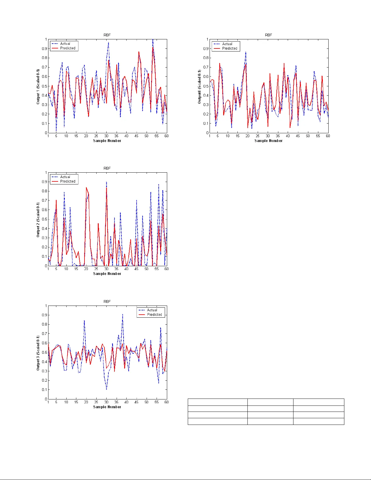
Abstract — This paper investigate s the use of dif ferent Artifi cial Intell igence metho ds to predict the values of several continuo us variables from a Steam G enerator. The objecti ve was to determine ho w the d if ferent arti fici al intel ligence metho ds perform ed in mak ing predicti ons o n the given dataset. The artif icial int ell igence methods ev aluated w ere Neural Netwo rk s, Suppo rt Vector Machines , and Adaptive Neuro -Fuzz y Inference Systems. The ty pes o f neural network s inv estigat ed were M ulti -Layer Pe rcepti on s, and Radial Basi s F unction. Bayesian and comm itt ee t echniques were appli ed to these neural netwo rks. Each of the AI methods considered was si mulated in Matlab. The result s of t he si mulations show ed that al l the AI metho ds were capable of predi cting the St eam Generat or data reasonably accuratel y. How ever, t he A daptive Neuro-Fuz z y Inference system ou t perform ed the other metho ds i n t erms of accuracy and e ase of implementati on, while st il l ac hieving a fas t execution ti me as well as a re asonable traini ng ti me. Index Term s — Artif ici al I ntell igence, F uz z y Logic, Neuro- Fuz z y , Neural Network s , Suppo rt Vector Machi nes I. I NTRODUCTIO N A rt ificial Int elligence (AI) m ethods ar e concerned w ith machi n es or co mputer sy ste ms th a t h a ve th e ability to “learn ” an d so lve prob l ems, and as a result exhibit “intelli gent” be ha vio ur. Norma lly , in telli gent be ha vio ur is assoc iated w ith char acteri stics such as h a ving th e ability to adapt , lear n n ew skills, an d fo r m complex r elationsh ips [1]. Th ere a r e sev eral ar tificial in telligen ce methods th a t h ave be en dev elo ped such as Neura l Netw o r ks, Suppo r t Vec tor Machi nes, an d Neuro- Fuzzy Sy stems. Th ese AI sy stems ha ve be en ut ilised in diff erent applicati ons f o r example: patter n reco gn ition, prediction of pr oc es s v a r iables, and various c o n tr ol applicati ons. Each of th ese m ethods h as diff erent a ppr oac h es to adapti ng an d l earn in g in order to emulate in t elligent be ha vio ur. Such Arti fic ial In telligence methods are par ticular l y usef ul i n mode llin g co mplex rela tionsh ips w h ere th e r elat ionshi p cann ot b e computed dir ectly or easily in terpr eted by a h uma n. A we ll kn ow n Ar tificial In telligen ce me th od is N eural Sch oo l of Ele ct rical and Inf orm ation Eng ine erin g P/Bag x 3, Wits , 2050 South Af ric a Web sit e: w w w.t sh ilidz imarw ala.com Netw orks. Neural n etw orks ar e in spir ed by t h e mec h an isms of th e h uma n b rai n and a re capable o f learn i n g co mplex rela tionsh ips th r ough th e assoc iati on of exampl es o f th ese rela tionsh ips [2]. A neur al netwo rk co n t in uous ly ada pts o r adjusts th ese co m plex r elat ionshi ps fo un d in an example dataset un ti l i t h as l earn t th e r elat ionsh ips suff i ciently we ll. Neural n etw o r ks model th ese co mplex r elati onships in term s of a set of f r ee par a meters (we igh ts an d biases) th a t can be math emat ically r eprese n ted b y a function [3]. Th ere ar e num erous ty pes of n eural netwo r ks th at can be impl emented such as Radia l Basis Function an d Multi-la y e r Perceptions. Suppo rt Ve cto r Machin es i s a more rece n t Ar tificial Int elligence m ethod dev elo ped by Vapni k an d his college s’ in 1992. Support Ve cto r Machin es ar e b ased on s tat istical lear ni n g w her e t he goal i s to determin e an un know n depe n dency be twe en a set of in puts an d outputs, an d th is depe n dency i s estimated from a li mit ed set of example dat a [4]. In the case of classif ication, t h e idea is t o co nstr uct a hype r-pl an e as a decisio n sur face i n such a w ay th a t th e mar gin of se par at ion be tw ee n th e dif fe ren t classe s is maxim ized [5]. In t h e class of function a ppr oximation, th e goal is to fin d a function th at h as at most a certai n dev iati on from the desired target for a ll t he points in a dat aset of exampl es used t o m odel such dependenc ies. Like n eural netwo rks, it mode ls c omplex r elationsh ips using a math emat ical a ppr oac h . Neuro-F uzzy Sy stems ar e based on Fuzzy logic which was fo r m ulated i n th e 1960s by Zadeh [6]. T h ese sy stems co mbine Fuzzy Lo gi c and certa in pr in ciples o f N eural N etw o r ks in order to mode l co mplex r elat ionsh ips. Fuzzy sy stems use a more l in guisti c appr oach ra th er th an a m ath emat ical appr oach, w h er e rela tionsh ips a r e desc ri be d i n n at ur al lan guage usin g lin guisti c varia ble s [6]. All of the AI methods m enti oned r equir e a da taset in o r der to tr ai n t h e AI sy stems t o be a ble t o mode l th e complex rela tionsh ips of t h e sy stem being modelled. Ther ef ore, th e AI sy stem lear n s by exampl e t h r ough a tra in in g proce ss, an d t hi s dataset i s called a tr ai n in g da taset. Mo st AI meth ods can be use d fo r function appr oximation in w hich predictions of co nti n uous vari ables can b e genera ted. In t h is pa per, t h e in ves tiga tion in t o ce r tain AI methods fo r t h e application of pr edicting certa in vari ables from a Steam Gener ator will be di scus sed. Th e AI meth ods th at we r e i n ve stigated we re: Neura l Netw orks (Radial Basis Artificial I ntellige nce T echniques f or S team Gener ator Modelling Sar a h Wrig ht a nd T shi li d zi Ma rwala Function, Mult i-Lay e r Perce ption, Committees, a n d Bay esian Techn iques), Suppo rt Vec tor Machin es, an d Adaptive Neuro- Fuzzy In fe ren ce S y stems. Each o f th eses AI meth ods w ere in ve stigated a nd simul ated in Matla b, in order to ascertai n th e perfo rm an ce o f each method a s we ll as its str engt hs an d w eakness w hen appl ied to th e stated a pplicati on. Th e m ain perfo rm an ce measures under co nsider ation a r e t he accura cy ob t ain ed, spee d of tr a in in g, an d th e spe ed of exe cution of t h e AI sy stem on un see n data . Th e pa per will first give a b asic fo un da tion o f th e th eory o f th e AI meth ods used, an d th en t h e i mplement ations a n d th eir results w i ll b e pr ese nt ed. Fin a lly , th e key findi n gs of th e simulat ions will be discus sed. II. T HE S TEA M G ENER ATOR D A TA SET Th e pr ob lem r equires mode lli ng th e i n put-output rela tionsh ip o f data o btained f r om a Steam Ge n erat or at Ab bo t t Pow er Pla n t in th e U SA. Th e da taset used is availa ble onlin e, a n d co n tai n s 9600 sampl es. Th e model co nsists of 4 in puts an d 4 outputs. Th e in puts a r e th e i nput f ue l, a ir , refe r ence l ev el (in ches), an d distur bance def in ed by th e load lev el. Th e f uel and a ir i n puts h ave be en scaled be twe en 0 a n d 1. Th e outputs ar e th e dr um pr essure (PSI), exce ss oxy gen i n exhaust gases (percentage), th e lev el o f water in th e dr um , an d th e steam f low (Kg/s). B oth th e in put s an d outputs ar e in num eric fo rm and have diff erent un i ts to expr ess their quan tit ies. T h e idea is to be able t o pr edict th e outputs fo r a spec ific set of in puts for th e steam generat or. Th erefo re, th e proble m is a r egr ess ion prob lem as th e go al is to pr edict th e value of a n umbe r of co nt in uous varia ble s. Th is data set will be mode lled using t h e di ff erent art ificial in t elligence m ethods menti oned abo v e. III. A RTIFICIA L N EURAL N ETW ORK S A. Gene ral Theory of A rtific ial Neural Netw orks Neural Netwo r ks we r e origin al ly in spir ed by th e mechan isms use d by th e h uma n b r ain to lear n by expe r ience an d pr oc esse s i n fo r m ation. T h e hum an bra in consists of man y in terconn ec ted n eurons th at fo rm an i n fo r m ati on pr oc ess in g netwo rk capab le of learn i n g an d adaptin g f r om experien ce [2, 7]. F igur e 1: Stru ctur e of a Gen era lised Artificial Neu ron [5] Basic ally, a n eur al n etwo r k i s a data mode llin g t ec h n ique used to fo r m an in put /output r elationsh ip fo r a spec ific proble m [2]. T h eref ore, an in put/ output relat ionshi p must exist fo r t h e n eural netwo rk to function i n pr edictin g outputs or classify in g dat a. T h e basic compo nen t of a n eural n etwo rk is a n a r tificial neuron which is a lar gely simpl ified repr ese nt ati on of a bio lo gical n euron. Each n euron r ece ive s a num be r o f in puts w h ich may b e from th e outputs o f other neur ons or th e source data being fe d in to th e netwo rk [2, 7]. Each i n put is mul tipl ied b y a we ight to dete r min e its in flue n ce or str en gth . T hese we igh ts a r e an a logo us to th e adjustment of th e sy na ptic co n n ections betw een n eurons t h at oc curs dur i n g th e lear n in g pr oc ess in b iolo gical sy stems [2, 7]. T h e w eighted in put s an d a n extern al bias value a r e summed. Th e summed sign al is passed t h r ough an activation function to pr oduc e the n eur on’s output sign al. T h e b ias value ha s th e e ff e ct o f increasin g o r dec reasin g the signal in put passed to th e activation function an d is simi lar to th e firin g th r eshold o f a biolo gical n euron [2, 7]. Th e activation function limits the amplitude ran ge of th e n eur on’s output signa l [5]. An ar ti fic ial neur on r epr ese nt s th e basic in fo r m ati on proce ssing un it of an y n eur al n etw o r k. H ow eve r, th e genera l char acteri stics o f th e ar tificial n euron: activation f unction used, biase s, meth od of calculat in g th e w eight s, an d n um be r of i n puts; w ill diff er depe n din g on th e ty pe of n eural n etw ork an d th e pr ob lem be in g modelled. Figur e 1 sh ow s t he m ode l of an ar ti fic ial neur on [5]. The gen eral mat h ematical mode l of a neur on can be des cribed b y Equat ion 1 [5]. + ∑ = = k j kj N j k b x w f y 1 (1) w her e: y k = output of th e kth neur on x j = th e jth in put w kj = we igh ti ng co n nectin g t he jth i n put t o neuron k. A n eura l n etw o r k co nsists of sev eral l ay ers of i n terconn ec ted ar tificial neur ons wo r ki ng together to model a pr ob l em. Th e ty pes of neur al netwo rks that will b e discuss ed ar e fee d- fo r ward neur al n etwo rks, meani ng th at th e signa ls can only tr ave l in one dir ection th r ough th e n etwo r k str uctur e: from th e in puts to w ar ds the outputs. Th e in put l ay er co nsists o f sev er al in put s (source data ) to be modelled by th e netwo rk, it doe s n ot h ave an y n eurons an d n o computation is perfo r med [5]. Th e n etw ork may ha ve seve ra l hidden lay er s th at in tr oduc e more adjustab le w eight in gs to t he netwo r k, allow in g a hi gh er order model of t h e data to be extracted [5, 3]. T h e fin al l ay er is t h e output lay er of th e n etw ork which produce s th e ove ra ll n etw ork’s outputs. Ea ch lay er of t he netwo rk r ece ive s in puts from the pr ev ious lay er o f th e netwo rk, an d pa sse s its outputs to th e n ext la y er . No rm all y , ev ery n ode i n a lay er is co nn ected to ev ery oth er n ode i n t h e fo l low i n g la y er (m eshed) [5]. Th e basic str ucture o f a f ee d- fo r ward n etw o r k can be se en i n Figur e 2 [5]. w kN w k2 w k1 X N X 2 X 1 Σ Bia s b k Activ a tio n Functio n f (.) Inpu ts Output y k k = Numbe r of Ne uro ns A neur al netwo r k learn s by example th rough tr ain i n g algorit h ms. Tra in in g r esults in an in put/ output r elati onshi p be ing determin ed f or a s pec ific prob lem. Tr ain i n g can be supervise d or unsupervise d. The neural netw o r ks discusse d w ill use supervise d tr ai ni n g. Supervised t r ain in g i n vo l ve s ha ving a t r ain in g da taset w her e n umerous exampl es of in puts an d th eir co rr espo n din g outputs (t ar gets) ar e fed t o th e netwo rk. Th e weights an d biases of t he n eural n etw o r k ar e co nti n uous ly adjusted to min imise th e err or b etw ee n th e netwo rk’s outputs a nd th e ta r get outputs [2, 5, 7]. F igur e 2: Basic Struc ture o f a F eed -forward Artificial Neur al Network [5] Opti misat ion techn iques can be used to de termi n e th e w eights of th e n etwo rk, sin ce it is a min im isati on pr ob l em. Th erefo r e, t h e kn ow ledge or i n fo r m ati on abo ut t h e prob lem is co nta in ed by t he we igh ts a n d biases of th e n etwo r k. An im portan t pr operty of n eural n etwo r ks is th eir ability to genera lise. General isation r efe rs to th e abilit y of th e n eur al netwo rk to predict or pr oduc e r easo na ble outputs fo r i n puts not seen dur in g the tr a in in g o r lear n in g pr oce ss [5]. T h us, th e in put/output r elat ionshi p co mputed is valid f or un see n data. General isation is in fluence d by t h e siz e of th e tr ai n in g da taset an d th e ar chit ec tur e o f th e n eural n etwo rk [5]. Th e be st genera lisati on is n orma lly a chieve d when t he n umbe r of free par ameters is fair ly smal l co mpar ed t o th e size of t h e da taset [3]. H ow ev er, a neur al n etw ork can h ave poo r gen eral isation if it is un der-t r ain ed (un der -fittin g) or ov er -tr ai ned (ov e r - fittin g). Ov er-tr ain i n g oc curs when th e n eural n etw ork fits th e tr ain i n g da ta perfec tly an d r esults with a function appr oximation or bo un dar y lin e t h at i s not smo oth but err a tic in n at ur e [3]. T he n etwo r k ef fec tively memorises th e data an d th erefo r e, h as poo r gen eral isati on on da ta n ot i n th e tr a in in g set. Also , a n eur al n etw o r k can be under-t r ain ed: t h ere ar e n ot enough free par ameters to suf f icientl y fo r m an in put /output rela tionsh ip t h at captur es the features of th e pr ob lem [3]. B. Mul ti-Layer Perception Multi Lay er Pe rception (ML P) n eura l netw orks a re a popular class o f fee d-f orw ar d n etw orks (Figure 2). Th ey w ere dev elo ped f rom t he m ath emati cal m ode l of th e n euron (Figur e 1), a n d co n sist of a n etwo rk o f n eurons or perce ptions [2]. An MLP netwo rk co n sists o f an i nput lay er (source dat a), sev eral hi dden l ay ers of n eurons, a n d an o utput lay er of n eurons. The hi dden la y er s an d th e output lay er can h ave dif fe ren t activation f unctions. Th ere ar e v ari ous ty pes of a ctiv ati on functions th at can b e emplo y ed. Th e activation function of th e hi dden neur ons must b e n onlin ear a nd ar e usuall y functions th at ar e diff erenti able [3]. Ty pically , th e h y per bo lic tan gent or logistic functions a r e used fo r th e a ctivation function of th e hi dden n eurons. Ho w ev er , t he output activation function may be l in ear . Cert ain activation functions ar e more appr opria te fo r diff e r ent ty pe s of prob lems, th eref ore, th e activation function needs t o be sele cted acc ordin g t o t h e prob lem. No rm all y , a lin ear output a ctivation f un ction is used fo r regr essio n prob lems as it does not lim it th e r a n ge of t h e output sign al [2]. A m ulti-l ay er pe r ce ption neur al n etw o r k represents a multi varia te non-l in ear fun ction mappin g betw e en a set o f in put an d output vari ables [3]. It h as bee n sh ow n t h at an y co nti n uous function can be mo delled acc ura tely with one hi dden la y er , pr ov ided th ere is a suff i cient n umbe r of h i dden neur ons [3, 5]. An MLP n etw ork with one h idden l ay er can be mat h ematicall y r eprese n ted by Equa tion 2 [3]. + + ∑ ∑ = = = ) 2 ( 0 ) 1 ( 0 ) 1 ( 1 ) 2 ( 1 k j i j i Ninput i A kj Nhidden j k w w x w f w f y (2) w her e: k = num be r of outputs y k = th e output at th e k th n ode j = n umber of h idden n eurons i = n umber of in put s f A = activation function of th e h idden n eurons f = activation function of t he output n eur ons x i = the in put from th e i th in put n ode w ji = w eight s co nn ectin g th e i nput with th e h idden n ode s w jk = we igh ts conn ec tin g th e h idden w ith th e output n ode s w 0j an d w 0k = biase s Th e co mplexity of t h e model is r elated t o th e n umber of hi dden un its, as th e n umbe r of free par a meters (weights an d biase s) available to adjust is di r ec tly pr opo r tiona l to th e num be r of h idden un its. Tr ain i n g in vo lve s co nti n uous ly adjusting th e values of th e w eights a n d biases to mi n imise the er r or b etw een th e netwo rk’s output a n d th e desired t ar gets. In it ial ly , t he we igh ts an d b iases ar e set to r an dom values, a n d t h en adjusted usin g an optimisation t ec h ni que. H o we v er, such optimisat ion techni ques ar e hi gh ly susc eptib le to f i n din g local min ima , an d th ere is no guar an tee t ha t a gl ob a l min i mum h as bee n fo un d [3]. Th e be st w ay to tr y an d a vo i d a solution th at is a loc al mi n imum i s t o tr ai n man y netwo rks taki n g th e b est netwo rk pr oduc ed. Ne uro ns Ne uro ns Inpu t La y er Hidde n La y er Output La y er C. Radial B asis Functions Radial Basis Functions ar e two -l ay er fe ed-f o rward n eur al netwo rks w i th the a ctivation function of th e h idden uni ts be ing ra dial basis functions [5]. T h e response of th e h idden lay er un it is depe nden t o n th e dista n ce a n in put is from th e ce n tr e r epresented by the r a dial basis fun ction (E uclidean Distan ce ) [2]. Ea ch r adia l function h as two par ameters: a ce n tr e an d a width. T h eref ore, th e ma ximum a ctivation of a hi dden unit is achieve d when the in put co in cides with th e ce n tr e ve cto r . Th e w idth of t he basis function determin es th e spread of t he function an d h ow quickly t h e activation of th e hi dden n ode dec r ease s with t h e in put b eing an i n creased distan ce f r om th e ce nt r e [3]. Th e mos t co mmon ra dial basis function used is th e Gaussian bell-sha ped distr ibution. No rm all y , a n RB F only h a s one h i dden lay er, an d a lin ear output la y er . Th e in put lay er sim ply pa sse s th e i n put data to th e h idden lay er. An RB F n etw o r k can be modelled math emat ically by Equat ion 3 an d the Gaussian activ ati on function is repr ese nt ed by Equa tion 4. Th e bias par ameters at th e output l ay er co mpensate fo r t he diff erence be twe en m ean output values an d mean t ar get values [3]. ( ) ( ) 0 1 k j kj M j k w w y + ∑ = = x x φ (3) w her e: y k = th e output at th e k th n ode M = num b er of h idden n ode s w kj = th e we igh t facto r from th e j th h idden n ode to th e k th output n ode w k0 = t h e b ias par ameter of th e kth output n ode φ (x) = radi al basis activation function − − = 2 2 2 exp ) ( j j j σ φ u x x (4) w her e: x = in put ve cto r u j = centr e ve cto r of th e jth h idden n ode σ = w idth of basis f un ction An R BF is tr ain ed i n tw o stages. T h e first stage i s a n unsupervised lear n in g pr oc ess to determ in e t h e pa r ameters of th e r adi al basis function for each hi dden n ode [3]. Th er ef o r e, only th e in put data is used dur i n g this proc ess . Th ese par ameters ar e th e centr es a n d th e w idth s o f th e basis functions. There are a n umber o f un supervised tr a in in g algorit h ms to determ in e t h e pa r ameters of th e basis f un ctions such as K-means clusterin g. Th e sec o nd stage i nvolv es findin g th e final lay er w eigh ts that mini mise t he e r ror be tw ee n th e n etw o r k’s o utput and t h e tar get values . Th erefo r e, t h e seco nd stage is done usin g supervise d lear n in g. Since the output lay er is a l in ear f un ction, the f in al lay er w eights can be solve d usin g li near al geb ra [3]. Bo th of th ese stages a r e r elat ive ly fast, th erefo re, a n RB F tr ain s much faste r th an a n equiv alen t MLP. Th e par a meters of an RB F can b e determin ed b y supervised t r ain in g. Ho w ev er , the optimisat ion proce ss is no lo n ger lin ear , r esultin g i n th e pr oc es s be in g co mputati onall y expe nsive compared to th e two stage tr a in in g proce ss. Th e ma in diff erence be twe en MLP s and RB Fs a r e t h at an MLP splits t h e i n put space i n to h y per-pla n es whil e an RB F splits t he i n put space in to h y per -spher es [2]. D. Committee s Comb ini n g th e o utputs of se ve ra l n eural netw orks in to a singl e solution t o gain im pr ov ed accuracy ov er an in dividual netwo rk output i s call ed a committee or en semb le [8]. Th e simplest w ay o f co mbing th e outputs of diff erent n etw o r ks toge th er is to ave r age th e outputs ob t ain ed [3]. Th e ave ra gin g ensemb le can be expresse d by Equati on 5 [3, 8], K i N i K y N y 1 1 = ∑ = (5) w her e y k i s t he kth output, y ki is th e kt h output of n etw ork i, an d N i s th e n umbe r of n etw o r ks in th e co mmit tee. It can be show n th a t averagin g th e pr edictio n of N netwo rks r educe s th e sum-of -squar es err or by a fac tor of N [3]. H o w ev er, th is doe s n ot ta ke in t o ac co unt th at so me netwo rks in th e co mmitt ee may gener ate b etter pr edictio ns th an others[3]. In th is case , a weighted sum can be fo rmul ated in w h ich certa in netwo rks co nt r ibute more to th e final o utput o f t he committee [3]. Th ere ar e seve ra l other committee m ethods to impr ov e th e accuracy of t h e pr edictio n ob t ain ed, such as Baggin g an d Bo ostin g. E. B ayesian Technique s for Neural Net w orks Th e tra in in g of th e neur al n etwo r ks usin g th e more stan dar d appr oaches r elies on t he min i misati on of a function err or (Maximum Likelihoo d Approach) [3]. This approach makes def in in g th e n eural netwo r k model diff icult, an d bo t h tr ain i n g and v alidat ion datasets ar e n ece ssary to determin e th e mo del th at exh ibits th e b es t ge n erali sation. There w i ll alway s b e a ce r tai n err or be tw ee n th e predicted and t h e actual. If seve ral n etw o r ks with i denti cal ar chi tectures are produce d w ith th e same err or, t h e we igh ts a n d biases will n ot be th e same each ti me, a s th ere is a leve l of un certai nt y in t he tr ain i n g pr oce ss due to t h ere be in g ma ny pos sib ili ties fo r par ameters. In t he Bay esian appr oac h , a pr ob a bility distr ibution function i s considered t o be r epr ese nt ed ov er th e w eight space , t o acc ount fo r the uncerta in ty i n deter min in g th e w eight vec tor [3]. In stead of attemptin g to find a sin gle set of w eights t h at min imi sed th e err or b etw ee n th e predicted an d actual v alues. The pr obab ility distribution r epresents th e degree of confide n ce asso ciated to th e diff erent values fo r th e w eight ve cto r [3]. Th i s pr ob a bility distr ibution i s in it ial ised to so me pr ior di stri butio n , an d th en w ith th e a id of t he tr ai n in g dataset t h e pos teri or pr ob ability di stri butio n can be determin ed an d used to ev aluat e th e pr edicte d outputs fo r n ew in put data po in ts [3]. Th e po sterior pr ob ability distr i butio n can b e expresse d using Bay es’ T h eo rem an d is show n i n Equati on 6. ) ( ) ( ) | ( ) | ( D P w P w D P D w P = (6) w her e D r eprese n ts th e ta r get values of th e tr a in in g da taset, w is the ve cto r r eprese nt in g the adaptive w eigh ts and biases , P(w ) is th e pr ob ability distr ibution function of t h e w eigh t space in a bs ence o f a n y dat a po in ts (Prior Prob ability Distri butio n ), P(D) is a n orm ali sation f actor, P(D |w ) i s a likelih oo d function, and P(w |D) is the posterior pr ob ability distr ibution. U sin g B ay e s’ Theorem a llow s a n y pr ior know ledge abo ut th e uncerta in w eight values to be upda ted base d on th e kn ow ledge gain ed from t h e tr ain i n g dat aset to produce th e po sterior distr i butio n of the un kn ow n w eight values [3]. Th e pos teri or pr ob ability distribution giv es an in dication of w h ich weight values fo r the we igh t vec tor ar e most prob able [3]. Th e pr i or pr ob a bility distr ibution should t ake in to acco un t an y in fo rm ati on kn ow n abo ut t h e we ight s [3]. From regula ri sation tec h n iques, it’s kn ow n th at smal l w eight values ar e fav o ur ed in order to pr oduc e smo oth netwo rk mappi n gs. Th erefo r e, the we igh t-decay r egular isati on n eeds to be in co rpora ted in t h e pr i or pr ob ability distr ibution function. For pri or prob ability di str ibution t h at is a Gaussian function, th e fo r m is show n in Equati on 6 [3], where W is t h e n umbe r of w eights an d Z w i s th e n orma lisat ion co ef f icient. If th e w eight dec ay ter m is sma ll th en th e p(w) is lar ge. Th e quan tit y α is th e co ef ficient of we igh t-decay . ( ) ) 2 ex p( 1 ) ( 2 w Z w P W α α − = (6) w her e 2 2 w W Z = α π Th e Likelihoo d pr ob ability distr ibution is given by Equati on 7, a n d is an expr ess ion of the diffe ren ce be twe en t he pr edicted output ( y(x,w ) ) an d t h e tar get output ( t ). Th e quan tit y β is th e co ef ficient of th e dat a er r or [3]. ( ) ( ) { } − ∑ − = = 2 1 , 2 exp 1 ) | ( n n N n D t w x y Z w D P β β (7) w her e 2 2 N D Z = β π Th e pos teri or pr ob ability distr ibution can b e ob tain ed b y apply in g B ay es ’ th eo rem an d is gi ve n be low [3]. It can be see n th at S(w) is depe nden t on th e sum-of -squar es err or function an d a weight r egular isation ter m [3]. ( ) ( ) ( ) { } ( ) ( ) dw E E Z w t w x y E E W S w S Z D w P W D S i W i n n N n W D S α β β α α β α β − − ∫ = ∑ + − ∑ = + = − = = = ex p , 2 , 2 ) ( wh ere 8 ) ( exp 1 ) | ( 2 1 2 1 Th e tr ain i n g pr oc ess fo r th e Bay es ian appr oach i n vo l ve s determin in g th e a ppr opriate po sterior pr ob ability di str ibution of th e we igh t values [9]. In order, to ma ke a pr ediction fo r a new in put ve cto r, t h e o utput distr ibution m ust be computed, an d is give n by Equat ion 9. T hi s E quation is eff e ctive ly takin g a n ave ra ge pr ediction of all th e mode ls w eight ed by th eir degree of pr ob ability [3], and is depe nden t on t h e pos terior prob ability di str ibution. Th erefo re, th e tr a in ed netwo rk can m ake pr edictio n s on in put data it h as n ot seen by using th e poste r ior pr ob ability distr i butio n . dw D w P w x y P D x y P n n n n ) | ( ) , | ( ) , | ( 1 1 1 1 + + + + ∫ = (9) Th e ev alua tion of th e prob ability distr ibutions requir es in tegra tion ov er a multidi mensiona l we ight space , an d is n ot easily ha n dled a na ly tically. On e meth od to ev a luat e t he in tegra ls is to use a Gaussian Appr oximation which all ow s th e in tegr al to be an aly ticall y ev aluat ed using optimisat ion techni ques [3]. Anoth er co mmon method used to solv e th ese ty pe of i n tegra ls i s a r an dom sam plin g meth od called Mo nt e Car lo Techn ique [10]. Ther ef o re, t he Mo n te Ca rl o or th e H y bri d Monte Ca r lo meth od is n orm ally used t o i denti fy t h e pos terior probab ility distr i butio n of th e we ight s fo r a Bay es ian neur al n etw o r k, by sampl in g from th e po sterior we igh t distr ibution. F. Monte Carlo Methods In t h e Bay esian appr oach to n eur al n etwo r ks, in tegra tion play s a sign i fic an t r ole a s calculat ions i n vo l ve evaluatin g an in tegra l ov er t h e we igh t spa ce . Monte Car lo is a meth od of appr oximatin g th e i nt egral b y usin g a sa mple of points from th e function of i nt erest [3]. Th e in tegra ls th at n ee d to b e ev aluat ed ar e o f th e f orm [3], dw D w P w F I ) | ( ) ( ∫ = (10) w her e F(w) i s th e integr an d an d P(w| D) is th e po sterior distr ibution of w eight s. T h is i nt egral can th en be appr oximated usin g a fini te sum of th e fo r m, ) ( 1 1 i L i w F L I = ∑ ≈ (11) w her e w i i s th e sample of we igh t ve cto rs genera ted from t h e pos terior pr ob ability distr ibution [3]. In order to gener ate samples of th e w eigh t vec tor space repr ese nt ati ve of th e P (w |D), a ra n dom search th r ough th e w eight space fo r a r eas we re t h e distr i butio n i s reasonably lar ge i s per fo r m ed. T h is do ne using a techn ique called Markov Ch a in Mo n t e Car lo, w h er e a seque n ce of w eight ve cto rs are genera ted, each n ew v ec tor in th e seque nce depe n din g on th e pr ev ious w eight v ec tor plus a ran dom co mponent [3]. A ra n dom w alk is th e simpl est method in w hi ch each suc ces sive step i s computed using Equation 12 [3]. ε + = + n n w w 1 (12) ε is a r a n dom ve cto r t h at al low s more of t h e we ight space to be explo r ed. In order , to find samples of weight ve cto rs th at ar e representa tive o f th e P(w |D) distr ibution, a proce dure know n as t h e Metropo lis A lgorit h m is used to sele ct t he sample we ight ve cto r s. Th e Metropo lis Algori th m r eje cts or acce pts a c erta in sample of the weight space or state genera ted usin g Equation 12 based on th e f o llow in g co ndit ions, ) | ( ) | ( y probabilit w ith st ate ac ce pt ) | ( ) | ( state ac ce p t ) | ( ) | ( if 1 1 1 1 1 D w P D w P w D w P D w P if w D w P D w P n n n n n n n n + + + + + < > U sing th e a bo v e co ndi tions, certa in of t h e w eigh t vec tor samples will b e rej ec ted if th ey lead to a reduction in th e pos terior distr ibution [3]. T h is pr oc edure i s r epeated a num be r of tim es un til th e n ec ess ar y n umbe r of samples ar e produce d for t h e ev alua tion of th e fin ite sum fo r t he in tegr al. Due to h igh corr elation in th e pos teri or distr i butio n as a r esult of th e each suc ces sive step being depe n dent on th e pr ev ious, a lar ge n um be r of t h e n ew we igh t ve cto r sta tes will be reje cted [3]. Ther ef o r e, a H y bri d M onte Car lo me th od can be use d in stead. Th e H y bri d Monte Car lo m ethods use s in fo rm ati on abo ut th e gr adien t o f P (w |D) to ensur e th at samples th r ough the ar eas of h igh er pos teri or pr ob abilities ar e fav oured [3]. Th is gra dient info rm ati on c an b e ob tain ed th r ough th e b ack- propagat ion algorit h m. Th e H y brid M onte Car l o method is base d on th e pr in ciples of H ami ltoni an mechan ics th at desc ri be molecular dy na mics [10]. It is a fo r m of the Mar kov Cha in , h ow ev er, th e t r an sition be tw ee n sta tes is ac h iev ed using th e stoc ha stic dy nam ic model [9]. In stati stical mechan ics, th e stat e space of a sy stem a t a certai n ti me can be desc ri be d b y t he pos iti on an d momentum of all th e molec ules of th e sy stem at tha t time [9]. The position def ines th e pote nt ial energy of t h e sy stem a n d th e momentum def in es t h e kin etic energy of th e sy stem [9-10]. T he total energy of th e sy stem is t h e sum o f t he potenti al and kin etic en ergy , a n d can be r eprese n ted by th e Hamilt o n ian equation def ined a s, 2 2 1 ) ( ) ( ) ( ) , ( i i p w U p K w E p w H ∑ + = + = (13) w her e w is t h e position var iable, p i s th e momentum varia ble , H (w ,p) is th e total energy of the sy stem, E (w ) is th e po tenti al energy , an d K(p) is t h e kin etic en ergy . Th e positions ar e an alogo us with the we igh ts of a neur al netwo r k, a nd potentia l energy with t h e n etw o r k er r or [10]. In th i s equation, th e energi es of t h e sy stem ar e def in ed by e n ergy functions repr ese nt in g th e s tat e of t he phy sical sy stem (can onical distr ibutions) [10]. In order to o btain th e po sterior distr ibution of th e n etw ork we igh ts, t h e fo llow in g distr i butio n is sam pled i gnor in g th e distr i butio n of th e mome nt um ve cto r [9]. )) , ( exp( 1 ) , ( p w H Z p w P − = (14) H amil tonia n dy na mics ar e used t o sam ple at a fixed energy in terms of a fic tit ious ti me τ [9-10], a nd ar e show n in Equati on 15 an d 16. Sin ce th e dy na mics show n in Equa tions 15 an d 16 can n ot be s imul ated e xactly , the equations are disc retised using fin ite time steps give n by E quation 17 a nd 19. [10]. In th is w ay th e position an d mome n tum at t ime τ + ε is expresse d in t erms of th e position a n d momentum at t ime τ [10]. T h is meth od is kn ow n as th e l eap-f r og m ethod. T h ese new states a re acc epted or reje cted usin g th e Me tr opo l is criter ion. i i i p p H d dw = ∂ ∂ = τ (15) i i i w E w H d dp ∂ ∂ − = ∂ ∂ − = τ ( 16) ( ) ( ) [ ] τ ε τ ε τ i i i i w w E p p Equations d Discre tise ˆ 2 ˆ 2 ˆ ∂ ∂ − = + (17) ( ) ( ) + + = + 2 ˆ ˆ ˆ ε τ ε τ ε τ i i i p w w (18) ( ) ( ) [ ] ε τ ε ε τ ε τ + ∂ ∂ − + = + i i i i w w E p p ˆ 2 2 ˆ ˆ (19) Th e basic steps in the im plementa tion o f th e Hy brid Monte Car lo algori th m ar e [9, 11]: (i) Ran domly choo se a tr ajec tory dir ection ( λ ) where λ i s -1 fo r a bac kw ar d t r ajec tory an d +1 fo r a fo rward tr ajec tory . (ii) Sta r tin g from a curr ent stat e (w , p). Perfo r m L l eapf r og steps w ith th e step size ε usin g E quations 16-19 to product a candida te stat e (w *, p*). Pe r fo rmi n g L leapf r og steps a llow s more of th e state space to b e explo red faster. (iii) Us in g the Me tr opo lis cr iter ion, a cc ept or r ej ec t th e (w*, p*) sta te. If th e candi date state is r ej ec ted the old sta te (w , p) is kept as the n ew state. Other w ise, th e c an didat e state is acce pted an d it bec o mes th e n ew state. IV. SUP PORT VECTOR MAC HINES Suppo rt Vec tor Machin es (SVM) we re int roduce d b y Vapni k an d hi s co lleges in 1992. T hey ar e base d on sta tisti cal lear ni n g th eo ry an d ar e one t y pe of kern el l earn i ng algorit h m in th e field of ma chin e lear n in g [4]. SVMs can b e used for bo t h classif ication an d r egressio n pr ob l ems. Th e goal of statisti cal lear n in g is to determ in e a n un kn ow n dependency be tw ee n a set of in puts a nd outputs, an d th is dependency is estimated from a l imi ted set of example da ta. [4]. Th erefo re, th e ob je ctiv e of a SVM, li ke n eural n etw o r ks, is to pr oduce a mode l which can pr edict th e output values of a da taset previo usly un seen. Th us, SVM s utili se supe r vise d lear n in g techni ques, an d r equir e a tr ai ni n g an d testin g da taset. In th e case of classif ication, t h e idea i s t o constr uct a hype r-pl an e as a decisio n sur face i n such a w ay th a t th e mar gin of se par at ion be tw ee n th e dif fe ren t classe s is maxim ized [5]. Th ese decisio n pl an es ar e def in ed t o act as dec ision bo un dar ies separat in g di ff er ent classes of ob je cts. F igur e 3: Sho wing a Linear SVM Reg ressio n for a Datase t Illustrating the ε -Tube a nd P ena lty Cost Function [ 12 ] In suppo rt vec tor r egressio n , t h e i dea is to find a function th a t ha s a t mos t a dev iati on of ε from the de sired targe ts for a ll the tra ining dat a ( ε -SV r egressio n) [12]. Thus, e rrors below the deviati on are not of concern, and point s outside this deviat ion are penal ize d (Refer to F igure 3). Theref ore, a function t hat a pproxima tes all the i nput-output pa irs with the define d precision m ust act uall y exist a nd the optimisat ion require d m ust be able to be fea sibly solved [12]. In order, t o acc ount for da ta point s t hat ca nnot be ea sily modelled, slack varia b les ar e n ormal ly in tr oduce d. In bo t h classific ati on an d r egressio n, th e i nput s ar e ma pped in to a h igh er dimensiona l feature space by a function φ (x) in duce d by a kern el function [4, 12]. Th e SVM th en fin ds a lin ear separat in g h y per-plan e w ith th e maximal margi n in th is hi gher dimensiona l space fo r t he classif ication case, a n d a se t of li near functions in t hi s h i gher dimen sional space fo r th e r egr ess ion case [4, 13]. T h ere ar e diff erent ty pes of kern el functions: l in ear, po ly n omial , radi al basis function (RB F), an d sigmoid. An y function t ha t sati sf ies Mercer’s Th eo rem can be use d a s a ker n el function [4]. T h e kern el function i s equal to th e in n er pr oduct of th e t w o vec tors (in put v ec tor ( x ) an d i nput pa ttern of th e ith tr ain i n g sampl e ( x i )) in duced in th e fe atur e space and is given by Equat ion 20 [5]. ) ( ) ( ) , ( i T i x x x x K φ φ = (20) In t h e c ase o f r egressio n, if given a tr ain i ng data set, {(x i , t i )} N i 1 = , where th e x is th e in put ve cto r an d t is th e tar get value, an SVM appr oximates th e function usin g Equat ion 21 [13]. b x w x f y + = = ) ( ) ( φ (21) w her e φ (x) r epr ese nt s th e h igh er dim ensional fe atur e space th at th e i n puts ar e ma pped t o, w is t h e we igh t v ec tor, an d b is th e b ias. Sin ce in r eali ty , n ot ev ery po in t w ill be a ble to fit w ith in th e dev iati on defined, th e Suppo rt Vec tor Machin e min im ises th e n umber of poin ts outside th e deviation usin g a penalt y par a meter [12]. T h is is achi ev ed by mi ni misin g Equati on 22. If Equa tion 22 is tr an sfo rmed in to dual fo r m ulati on, it is expresse d i n term s of th e kern el function an d support v ec tors. Support v ec tors consist of th e data poin ts th at sit o n the b oundar ies of th e acce ptable r egio n def i n ed by ε an d ar e extracted f r om t he tr ai n in g data set [5, 13]. Th i s co nstr ai n ed o ptimisat ion pr ob lem c an be so lve d usin g quadr ati c pr ogram min g w ith th e tr a in in g data a n d, as a result, is guar an teed to f in d a gl ob a l optimum [5, 12]. ( ) * 1 2 2 1 i i N i C w : Min imise ξ ξ + ∑ + = (22) 0 , ) ( ) ( * * ≥ + ≤ − + + ≤ − − i i i i i i i i t b x w b x w t : to Su bj ect ξ ξ ξ ε φ ξ ε φ w he re w - w eight ve ctor C - penal ty parameter N - number of data points ε - devi ation from funct ion i ξ , * i ξ - Sl ack Variables Th e c onstr ain t s abo ve deal w i th a lin ear ε -in sensitive los s function used to pe n alise th e data point s in th e tra in in g dataset th at ar e o utside th e spe cif ied de viation ε . A loss function is used to determin e which f un ction (f (x)) best desc ri be s t he dependency ob se r ve d in th e tr ai n in g da taset [4]. Th e purpose of th e loss function is t o dete r min e th e co st of th e diff erence be twe en the actual an d predicted outputs fo r a give n set of in put s. Th e ε -in sensitive los s function i s def in ed by Equati on 23 [4, 5]. A s see n in F igur e 3, in regressio n proble ms a ε -tube is f ormed ar ound th e function, an d an y data poin ts outside th is ε -tube ha ve an asso ciated co st gi ve n by Equat ion 23. Most data po in ts should la y withi n th e ε - tube , h ow ev e r , the sla ck var iable a llow some dat a poin ts t o l ie outside th e ε -tube [5]. Ther e ar e t w o sla ck vari ables t o acco un t fo r the upper an d l ow er bo un ds of th e ε -tube . Bo th ε a n d C ar e user-defined pa r ameters. Th e pa r ameter C is a regula ri sation par a meter th at co n tr ols th e tr ade-o ff betw e en th e co mplexity of t h e m achin e an d th e num be r of data points th at lie outside th e ε -tube [5]. Th e dev iati on ε , determin es th e appr oximati on acc uracy enfo r ce d o n the tr ai ni n g da ta points [13]. For r egressio n , the pa ra meters C an d ε should be tun ed simult an eo usly [5]. ( ) > − − − = oth erwise t x f if t x f t x f 0 ) ( ) ( ), ( ε ε l (23) Th ere a r e oth er ε -in sensitive loss functions th at can be used such a s a quadr ati c ε -in sensitive loss function. Also, a l east squares co st f un ction can be us ed. Th i s r esults in a Least Squares Suppo rt Vec tor Machin e (LS-S VM) th a t h as a f ew diff erent pr operties to th e origin al Vapn ik’s SVM pr esented abo v e. In a least squares SVM, th e ε -in sensitive loss function i s repla ce d by a least squar es cos t fun ctio n which co r r espo n ds t o a f o r m o f ridge r egressio n [14]. The in equality constr ain t s th at Equat ion 22 is subj ec t t o are replaced by equality . As a co nsequence , th e tr a in in g pr oc es s of a LS-SV M in vo l ve s so lving a set of lin ear equati ons in stead of a qua dr atic progra mmi n g pr ob lem. T he set o f lin ear equations th at r esult ar e of th e dimension N+1, w h ere N i s th e n umber of tr ai ni n g samples [15]. In t h e case of a stan da rd SVM, th e quadr at ic progra mmi n g (QP ) prob lem to b e so lv ed is r oughly expo nen tial to t h e siz e of th e tr a in in g da taset [14]. Th erefo re, th e n umber of t ra in in g sampl es used to tr ain an SVM should be co nsider ed carefully . Ho wev er , th e set of lin ear equations is still n ot as t ime an d co m putat ional ly co nsumi ng to solv e a s th e QP prob lem. In a LS-SVM , th e we igh t ve cto r t h at r esults from min im izi ng th e summed squar ed a ppr oximation err or ov er all tr ain i n g samples is se ar ched fo r , w h ere th e approximati on err or is th e diff e r ence b e twe en th e SVM ’s o utput a n d th e desired tar get output [15]. Th e equation fo r a L S-SV M is show n be low in E quation 24 [15]. 2 0 2 2 1 i N i e C w : Minimise = ∑ + (24) i i i e b x w t : to Subject + + = ) ( φ w he re e i = t i - f(x i ) Th e ma in diff erence be tw ee n Neura l n etw orks an d Suppo rt Vec tor Machi n es is t h at suppo rt ve cto r ma chin es min i mise an upper bo und of th e gener ali sation err ors in stead of min im isin g the e rr or o n th e tr ai n in g dataset [13]. Suppo rt ve cto r mach in es utilise r isk m in im isation, m easured usin g a loss function. No rm all y , suppo rt v ec tor machin es h a ve a slow er exe cutio n ti me as t her e is li ttle contr ol ov er the num be r of suppo rt ve cto rs def in ed [5]. An SVM h as less par ameters t o t un e tha n a neural n etw ork, a n d th e optimisation pr oc edure can be per fo r m ed ef fic ient ly . In th e case of th e LS-SVM , the pa r ameters t ha t n eed to be tun ed ar e th e pen alt y or regular i sation co n sta n t a nd th e deviation o f th e Gaussian fun ctio n , if an RB F ke rn el is used. Whil e f o r a stan dar d SVM th e ε a ccuracy fo r th e ε -in sensitive lo ss function n eeds to determi n ed additi onall y . V. FUZZY LOGIC A ND NEU RO-FUZZY SYSTEMS Neuro-F uzzy S y stems are b a sed on Fuzz y logic which was fo r m ulated in th e 1960s by Zadeh. These sy stems co mbine Fuzzy Lo gi c and certa in pr in ciples o f N eural N etw o r ks in order to mode l co mplex r elat ionsh ips. Fuzzy sy stems use a more l in guisti c appr oach ra th er th an a m ath emat ical appr oach, w h er e relat ionsh ips a r e desc ri be d i n n at ur al lan guage us in g lin guistic var iables. Fuzzy L o gic can deal w ith i ll-defined, im pr ec ise sy stems [16], a n d th er ef o r e ar e a goo d t oo l fo r sy stem m ode llin g. Th is sectio n in t roduce s th e basic s of Fuzz y Lo gic an d th en explai n s Adaptive Neuro- Fuzzy In fe r ence Sy stems th at ar e b ased on t h e fo un dations of Fuzzy Lo gic. A. B asic Fuzzy Logic Theory Fuzzy logic is a m ethod of mappi n g an in put space to a n output space by means of a list of lin guisti c r ul es th a t co nsist of if -th en sta tements [6]. Fuzzy logic co n sists of 4 co mponents: fuzzy se ts, membe rsh ip functions, fuzzy logical ope ra tors, a n d fuzzy r ules [6, 17, 18]. In classical se t t h eo ry , a n ob je ct i s eith er a member or i s not a membe r of spec ific set [17-18]. Th erefo re, it is po ssib le to determin e if an ob je ct belo ngs to a spec ific set a s a set h a s clear distin ct bo un dar ies, pr ov ided a n ob je ct can n ot achi ev e par tia l memb ershi p. Another w ay of th i n kin g abo ut t h is i s th at th e ob je ct’s be longin g t o a set is either tr ue or false . A char acteri stic function fo r a classical set h as a value of 1 if th e ob jec t b elo ngs to the set an d a v a lue of zer o if th e ob jec t doe sn’t belo ng t o th e se t [17]. F or e xample, if a s et X is def ined to r eprese n t all poss ible h eigh ts of peo ple, one could def ine a “tall ” subs et f or an y per so n w h o is abo ve o r equal to a spec ific h eight x , an d a n y one be low x doesn’t be long to t h e “tall” set but to a “ short ” subse t. Th is is clear ly in flexib le as a person just be low th e bo un da ry is l abe lled as be ing sh ort w hen th ey ar e cle ar ly tal l to so me degree. Th eref ore, in term ediate values such as f air ly t all a r e n ot al low ed. Also, th ese clear cut defined bo undar i es can be ve r y sub je ctiv e in terms of what a person may def in e as be longin g to a specif ic set. Th e ma in aim be hi n d f uzzy l ogic is to a llow a more fle xible r epr ese nt ati on of se ts of ob je cts by usin g a fuzzy set. A fuzzy set do es not h a ve as cle ar cut bo undar i es a s a classical set, an d th e ob je cts ar e ch ar acteri zed by a degree of membe rsh ip to a spec ific set [17-18]. Th erefo re, in ter mediate values of ob j ec ts can be represented which is close r to th e w ay th e huma n bra in t h in ks oppo sed t o t h e clear cut-of f bo un da ri es i n classical se ts. A m emb ersh ip function defines th e degr ee th at an ob je ct be longs to a certa in set or class. Th e membe rsh ip f unction is a curve that maps th e in put space varia b le to a n umbe r be twe en 0 an d 1, r epresenti ng th e degree th at a spec ific in put vari able belo ngs t o a spe cif ic set [17-18]. A membe rsh ip function can be a cur ve of an y sha pe. Us in g th e exampl e a bo ve, ther e wo uld be tw o subs ets one fo r tall an d one fo r short tha t w ould o ve rl ap. In t h is way a person can ha ve a par ti al par t icipati on in each of t h ese sets, th erefo re, determin in g th e degr ee to which th e person is both t all an d short. Lo gical operators ar e defined t o genera te n ew fuzzy se ts from t h e existin g f uzzy sets. In classical set th eory th ere ar e 3 main ope rat ors used, allow i n g lo gical e xpressions to be def ined: in t ersec tion, un ion, an d t he co mplement [17]. Th ese ope ra tors ar e used in f uzzy logic, an d h ave be en adapted t o deal with par tia l membe rsh ips. Th e in tersection (AND ope ra tor) of two fuzzy sets is give n by a m in imum ope ra tion, an d t he un i on (OR operat or) of two fuzzy sets i s gi ve n by a maxim um ope r ati on [17]. Th ese logical o perat ors ar e used in th e r ules an d determi n ati on of th e fina l output fuzzy set. Fuzzy Rules f orm ulat e the co ndi tional statement s w hi ch ar e used to m ode l the i n put-output relationsh ips o f th e sy stem, and ar e expresse d in n atur a l lan gua ge [6]. T h ese lin guisti c r ules ar e in th e f orm of if-then stat ements w h ich use the logical ope ra tors an d membershi p functions to produce an output. An i mporta nt pr operty of fuzzy logic is th e use of l in guistic v ar ia ble s. Lin guistic varia ble s ar e varia ble s th at take wo rds o r sentences as th eir values in stead of num be rs [17] . E ach lin guistic var iable t akes a l in guistic value th at corr espo n ds to a fuzzy set [17], a n d th e set of values th at it can t ake is called t he t erm se t [18]. Fo r example, a lin guisti c var iable Height could h a ve th e fo l low i n g ter m se t { very tall , tall , medium, short, very short} . A singl e fuzzy rul e is of th e fo rm : if x is A t hen y is B (25) w her e A an d B ar e fuzzy se ts def in ed fo r t h e i n put a n d output space r espe ctive ly . Bo th x an d y ar e li ngui stic vari ables , whil e A an d B a re th e lin guistic values or labels r epr ese nted by th e membe rsh ip functions [16]. Ea ch r ul e consists of two par ts: th e a n tece dent a n d th e co n seque nt [17]. Th e an tecede nt is t he co mponent of th e r ule falli ng be twe en the if-then, an d m aps th e in put x to th e fuzzy set A, usin g a membe rsh ip function. Th e co nsequent is t h e compo nen t of th e r ule a fte r th e th en , an d m aps th e output y to a membe rsh ip function. Th e in put membe rsh ip values act like we igh ti n g f a cto r s to determin e th eir in fluence on th e fuzzy output sets [17]. A fuzzy sy stem co nsists of a l ist of t h ese if-th en r ules which ar e evaluated in par all el. Th e an t ec ede n t can h ave more th an one l in guistic varia b le, t h ese in puts ar e co mbined usin g th e AND ope ra tor. Each of th e r ul es is ev alua ted f or an in put set, an d co rr espo ndi n g output fo r the r ul e ob tain ed. If a n input co rr espo nds to two l in guistic v ar ia ble values th en th e r ules asso ciated with bo th th ese values w ill be evaluated. Also , th e rest o f the r ules w ill ev a luat ed, h ow ev e r , will n ot ha ve an ef f ec t on th e fin al r esult as t h e l in guistic varia ble w ill ha ve a value of z ero. Therefo r e, if t h e an tece dent is tr ue t o so me degree, t h e conseque nt w ill h a ve t o be tr ue t o some degree [17]. Th e degree of each l in guisti c output value i s t h en co mputed b y per fo r m in g a comb in ed lo gical sum fo r eac h membe rsh ip function [17]. After which a ll th e co mbined sums fo r a s pec ific lin guisti c vari able can b e aggr egated. Th ese l ast stages i n vo l ve th e use of a n i n fe ren ce method w hi ch w ill m ap th e r esult o n to an output membe r shi p function [19]. Fina lly , a def uzzification proce ss is pr ef o rm ed in which a sin gle n umeri c output pr oduce d. On e method of co mputin g t h e degr ee o f each lin guisti c output value is to take th e maximum of a ll r ul es de sc r ibing t hi s li n guistic output value [17, 19], an d th e output is t aken as th e ce n tr e of gra vity of th e a r ea un der th e eff e cted par t of th e output membe r shi p function. Th ere ar e oth er in fe ren ce m ethods such as ave r agin g an d sum mean square [19]. Figur e 4 s h ow s the steps i n vo l ve d i n creatin g an in put-output mappin g usin g fuzzy logic [20]. Th e use of a se ri es of fuzzy rul es, an d i nference m ethods to produce a de fuzzifie d output co n sti tute a Fuzz y In fe r ence Sy stem (FIS) [21]. T h e final m an n er in w h ich th e aggr egation pr oc ess takes place a n d th e m ethod of def uzzification can di ff er dependin g on th e im plementa tion of th e FIS chos en. Th e appr oach discus sed abo ve is t h at of th e Mamdan i base d FIS. F igur e 4: Sh owing the Steps Invo lved in the Applica tion of F uzzy Logic to a P rob lem [20] Th ere ar e sev er al ty pes of fuzzy inference sy stems which vary acco r di n g to th e f uzzy r easonin g an d th e fo rm of th e if-then statements applied [16]. An other meth od o f Fuzz y in fe ren ce th at is w o r th discus sin g i s t he Takagi -Sugeno-K an g meth od. It is simil ar to th e Mamdan i appr oac h desc r ibe d abov e exce pt th at t he co nsequent par t i s of a diff erent form an d as a r esult th e def uzzification pr oc edure is diff erent. T h e if-then statement of a Sugeno fuzzy sy stem expresse s t h e output of each r ul e as a function of th e in put v a r iables, an d h as th e fo r m [1], if x is A AND y is B then z = f(x,y ) (26) If th e output of each r ule is a li n ear comb ina tion of th e in put varia b les plus a co nsta n t, th en i t is know n as a first-order Sege no fuzzy mode l, an d h as th e fo rm [1]: z = px + qy + c (27) Altern at ive ly , t he output of a rul e can be a constan t. Th e fina l output o f th e Suge n o FIS is a w eighted a ve ra ge of th e outputs from eac h r ule [16]. B. A daptive Ne uro-Fuz zy Infe rence Systems Th e mai n diff iculties w ith Fuzzy In fe r ence Sy stems ar e th at it is diff icult to tr an sfo r m h uman know ledge in to th e neces sar y rul e base , as we ll as to adjust t h e Memb ersh ip functions to ac h iev e a min imi zed output e rr or f or the FIS [16]. The purpose o f an ANFIS (Adapt ive Neuro-F uzzy Inference Sy stem or Adaptive Netw ork-Base d Fuzzy Inference Sy stem) is to estab lish a set of r ules along w ith a set of suitable memb ershi p functions t h at is c apable of repr ese nt in g th e in put/ output r elati onshi ps of a give n sy stem [16]. An ada ptive n etw ork r ef ers a mult i-laye r fee d-f orw ar d t y pe structur e with int erconnect n ode s. H o w ev er, so me of the nodes ar e ada ptive, m eanin g t ha t such a n ode’s output is depe n dent o n sev er al par ameters b elo ngi n g to it [16]. The lin ks in an ada ptive netwo r k o n ly in dicates t he f low of in fo rma tion. An ada ptive n etw o r k uti lizes a supervised lear ni n g a lgorit h m in o rder to m in imi ze th e e rr or o f th e in put/output m appin g r equired, by adjustin g t h e par ameters of th e adapt ive n ode s [16]. Th erefo r e, a tr ain i ng dat aset is neces sar y as th e tr a in in g pr oc es s is simila r t o th at used by neur al n etw orks exce pt th e par am eters of t h e adapt ive nodes ar e b eing adjusted in stead of th e we igh ts of th e li nks in th e netwo rk. An ANFIS is a ty pe of ada ptive n etw o r k with th e adaptive nodes r epresentin g membe r shi p functions and t h e conseque nt equations along with t h eir correspondin g par a meters [1]. Th e goal of a n ANFIS is to adjust th e memb ersh ip functions’ an d co nsequent equations’ par am eters to emulat e t h e i n put/output rela tionsh ips of a gi ve n da taset [21]. Th erefo re, an ANFIS is functionally equivalent to an FIS exc ept th at i t h as th e abilit y to learn an d adapt th r ough a tr ai n in g proce ss usin g i n put- output data pai r s to disco v er th e m os t a pproximat e par ameters of th e FIS to model th e sy stem accura tely . Th e basic a r chit ec tur e of a first-order Sugeno (T akagi -Sugeno- Kang) ANFIS with 2 in puts an d 2 r ules is sh ow n in Figur e 5 [1, 16]. F igur e 5: Sh owing the Arch itectur e of Fi rst-Ord er Su ge no ANF IS [1, 16] In F igur e 5, Lay er 1 co n tain s a seri es of membership functions w hich de termi n e th e degree th at th e give n input be longs to th e specif ic f uzzy set [16]. Th e membe rsh ip function’s par am eters ar e c ha n ged, th er ef o r e, cha n gin g th e F u z z y L o g i c Assignme nt o f Me mbe rship Fun ctio ns Appli cati o n Fu zzy Rule s Aggre gat e d Outpu t De fuzzificat io n Inpu t Va ria ble s Nume ric Output shape of t h e function an d t h e degree of membe rsh ip o f th e in put to a specif ic fuzzy set. Th e n odes in th is lay er ar e adapti ve an d th e par am eters ar e kn ow n as pr emise par am eters [1]. In Lay er 2, each n ode produc es th e product of th e in co min g signa ls. T h us, determi n in g th e fin al value or firin g str ength of eac h r ule [16]. Th e n ode s in Lay er 2 ar e fixe d, norm all y perfo rm in g a fuzzy AND ope rat ion. Each node in Lay er 3 calculat es th e n orma lized f iri n g stren gth by ta kin g a rul e’s firin g str ength ens an d dividing it by th e sum of al l t he r ules’ firi n g str engt hs [16]. Lay er 4 i s an adapti ve lay er th at h as a n ode f un ction equal to th e norm ali zed f ir in g str ength mul tipl ied by t h e f ir st-order Sege no fuzzy m ode l function. The f ina l lay e r (lay er 5) calculates th e fin al output by summ in g all th e in co min g signa ls [16]. Sin ce th e n orma liz ed fir in g str engt h an d fir st- order function ar e th e in co min g signa ls f r om the pr ev ious lay er, th e output of laye r 5 is eff ective ly a we igh ted a ve ra ge. All t h e respec tive equati ons can be fo und in [1]. An ANFIS is tr a in ed usin g eith er b ack-propagati on, or a hyb r i d tr ain i ng a lgorit h m (a co m binat ion of least squar es an d bac k-pr opagation). VI. I MPLEMEN TATION A ND RESULTS Each o f th e Ar tificial In t elligence methods discuss ed a bo ve w ere i mplemented using MA TLAB . In th is sec tion, th e implement ati on, r esults an d ob servations fo r each of t h ese methods will b e discusse d. Also , th e pr e-pr oc es sin g perfo rm ed o n th e Steam Generat or dat aset is di scus sed A. Data Pre-processing Be f ore a n eural n etw ork, SVM, an d Ne ur o-F uzzy Sy stem should be impl emented, th e dat aset n eeds to be a n aly sed an d proce sse d t o in sure th e be st possib le cha nce of a cquiri ng th e in put-output r elationsh ip of th e dataset. Pr e-proc ess in g th e dataset th at w ill b e fe d i n to th e n eur al n etw ork or AI sy stem is ve ry im portan t to t he performan ce, genera liz ation ability , an d t he speed o f tra in in g of th e n eural n etwo r k [3]. On in spectio n of t h e da taset, i t was see n tha t t h ere we re n o data po in ts with missin g values but th ere we re a n umbe r of outliner s. An outlin er i s a n extr eme point t h at does n ot seem to belo ng to th e dat aset an d m ay h ave an un justif ied in fluence on th e model [22]. Since two of th e in puts w ere alr eady scaled be tw ee n 0 an d 1, an y samples th at h ad a value gr eater th an 1 or less th an z ero f or either of th ese scaled i n puts w e r e co nsider ed to b e o utli n ers. T h e outliner s we re simpl y r emo ve d from th e dataset. Th ere we r e 965 outlin ers i n th e dat aset. Scaling of th e data is importa n t in neur al n etw orks a nd SVMs to equaliz e the im portan ce of each var iable [22]. Sin ce diff erent var iables c an have v a lues th at diff er in o rder s of magn it ude, t h e varia bles w ith th e lar ger values will appear more sign ificant in determin in g t h e o utputs [3]. Th us, a ll in puts should be sc aled to h a ve the same ra n ge. Also, scalin g is impo rt an t as th e activation f un ctions in neur al n etw orks only h ave a lim ited r an ge bef ore satur ation oc curs. Bo th th e in puts and the o utputs w ere scaled betw een 0 an d 1 usin g Min-Max n orma liza tion t o allow each var iable to h ave equal importa n ce . Min-Max n ormal iza tion uses t h e maxi mum an d min im um value of th e varia ble t o scale it to a r an ge b etw ee n 0 an d 1, an d is give n by E quation 28 [22]. Th e outputs can be co nverted back to t he o r igin al sc ale with out an y loss of accuracy . mi n max mi n x x x x x Scal ed − − = (28) Durin g th e collec tion o f th e dat a, th e sam ples can be stored in a spec ific o r der . Th e data set sto red th e samples in t h e seque nti al order in w h ich th ey w ere captur ed. Th erefo re, th e samples we r e r an domized i n order to break th i s spe cif ic order. Sin ce litt le else w as know n a bo ut th e da ta, n o other pre-pr oc ess pr oc edures w ere perfo rm ed on th e dat a points. Th e next step in t h e pre-proce ssing was to par tit ion the dataset into 3 datasets: trai n in g, v ali dati o n , an d a t esting dataset. Each dataset sh ould contai n a f ull r eprese n tat ion of th e available values . T h e tr ain i n g dat aset is used dur in g t h e supervise d tr ai ni n g pr oc ess to adjust th e we igh ts an d biase s to min im ize th e err or b etw ee n th e netwo rk’s o utputs and the tar get o utputs as w e ll as f or th e tr ain i n g o f t h e SVM an d neur o-f uzzy sy ste m to adjust t h eir corr espo n di ng pa r ameters. Th e validat ion data is used to per iodically ch ec k th e genera liza tion abilit y of t h e n etw o r k, SVM, or n euro-f uzzy sy stem. Th e validati on dataset is eff ective ly pa r t of th e tr ain i n g pr oce ss as i t is used to gui de th e sele ction of th e AI sy stem. Th e test dataset is used as a fin al measur e to see h ow th e AI sy stem perfo r ms on un seen da ta, an d should only be used once. T h e r esultin g dataset h as 8635 r eco rds of in put - output sets which we r e divided in to t h e 3 dat asets m enti oned abo v e. Th e sam e 3 da tasets w ere used fo r the im plementa tion of th e n eural n etwo r ks, th e SVMs, an d t h e ANF IS. B. Performance Me asures Th e mai n perfo r man ce measure tha t w as ut ili sed to ev aluat e th e pr edictio n ab ilit y o f th e Ar tificial In telligen ce Meth ods w as t h e Mean Squared E r ror (MSE). T h e Mean Squared Er r or is give n by Equati on 29. Th is equati on a llow s th e co ntr i butio n of each output to th e total MSE t o b e calculated. ( ) ( ) − ∑ ∑ = − ∑ ∑ = − ∑ = = = = = = 2 1 1 2 1 1 2 1 ) ( ) ( 1 ) ( ) ( 1 ) ( ) ( 1 k y k t R k y k t R k y k t R MSE p p R k m p p p m p R k R k (29) w he re R = size dat aset m = number of outputs y = predi cted val ue t = desired target value Other perfo rm an ce me asur es that w ere c onsidered ar e: the time t aken to tr ain th e AI sy stem, th e tim e ta ken to exe cute th e AI sy stem, an d t h e co mplexity of th e model pr oduc ed by th e AI meth od. C. Neural Netw orks Using Standard A pproaches Th e n eura l netw orks we re impl emented usin g th e open so urce NETLAB Too lbo x by Ian Nabney . Bo t h t h e MLP an d RB F n eural n etw o r ks were im plemented usin g th e stan dar d appr oaches with th i s too l bo x. Th e too lb ox only co n str ucts a 2 lay er fee d-f orw ar d n etwo rk f or bo th th e ML P an d RB F. Th erefo r e, t h ere is onl y o n e hi dden l ay er, an d o n ly t he num be r of h idden n ode s needed to be de term in ed. Th e in iti ali sation of th e MLP a n d RB F n etw orks in vo lve s determin in g th e a ctivation functions used an d th e siz e of th e hi dden la y er . A lin ear output activation function is be st fo r regr essio n pr ob lems, th erefo r e, it w a s util ised fo r b oth the MLP an d RB F. In t he case of an MLP, a l in ear output activation f unction do es n ot s atur a te, and as a r esult can extra po lat e a l itt le be y o nd th e t r ain in g dat aset [2]. Ho w ev e r , th e h idden n odes can satur a te which is one r easo n t he in puts an d outputs we r e scaled. In NETLAB , th e hidden n ode s of th e MLP ar e th e hy perbo lic tan gent. Th e hi dden n ode s o f th e RB F used th e Gaussian function as seen i n Equa tion 4. Th e gener ali sation ability o f a n etwo rk is determi n ed main l y by th e co rr ect mode l co mplexity and t h e n um be r o f tr ain i n g cy cles . Th er e a re a n umber of meth ods to impr ov e th e gener ali sation ability o f a n etwo r k such a s determ in in g th e mode l complexity , ear ly stopping, a nd r egular isati on. • Mo del complexity is r epr ese nt ed by th e n umber of hi dden n odes in th e n etw ork, a s th e h idden n ode s ar e responsible fo r th e n umbe r of a djustab le pa r ameters available i n th e n etwo rk [ 3]. T h eref ore, a more co mplex mode l h a s a gr eater n umber of h i dden nodes. Ho wev er , if t her e ar e too m an y h idden n odes th e sy stem w ill be un neces sar ily complex an d pr one to mode lli n g t h e sy stem’s da ta too w ell (ov er -fitted). Conve rsely i f th ere a r e too fe w hidden n ode s the netwo rk will n ot b e ab le to adequately mo del th e sy stem (un der-fitted). One way to determ in e th e optimal number of h idden n ode s i s to t r ain th e neur al n etwo rk with di ff er ent n um be rs of h idden nodes, a n d ob serve t he t ra in in g an d validat ion er rors ob t ain ed. Note th at a lar ge n umber of h i dden nodes w ill slow th e tr ai n in g pr oce ss. • Th e Ear ly Stopping techni que uses a tr ain in g as w ell as a v ali dati on dat aset. T h e main idea behin d ear ly stopping i s th at th e t r ain in g err or of th e n etw ork will gra duall y dec rease as t he n um be r of tr ai ni n g cy cles in creases. Th e degree th e n etw ork i s ov er-tr a in ed is measured usin g th e validati on dat aset as th e validation err or w ill decrease at first an d th en star t to in crease as th e n etw ork is ov er -tr ai ned [3]. Th erefo r e, tra in in g should be s toppe d at th e point be f ore th e validation err or be gin s to in crease. • Re gular isati on techn iques en co ura ge we igh ts t h at produce smoother n etw ork mappi ngs. An ov er-fitted netwo rk models the tr ain i n g data almost exactly , resultin g in th e m appin g pr oduc ed by th e n etw o r k ha ving ar eas of l ar ge cur vature [3]. Th is r esults in lar ge we igh ts. T h e simplest r egular isation t ec h n ique uses a we igh t-decay w h ere mappin gs with la r ge w eights ar e penal ised [3]. Regular isation pr eve nt s ov er -tr ai ni n g. Th e n umber of in puts an d outputs ar e determin ed by th e proble m, a n d as stated th ere ar e 4 i nput s an d 4 o utputs i n th e sy stem b eing modelled. Determin i n g t h e n umbe r o f h idden nodes used i s an i tera tive an d expe ri menta l pr oce dure, as it is depe n dent on the complexity of the r elati onshi ps in t he dataset. A r ough estimate f or th e n umbe r of hi dden nodes is to t ake hal f th e sum of th e t otal n umber of in puts and o utputs [2]. T h eref ore, 4 hi dden n odes w ere used as a sta r tin g point an d progressiv ely i n creased w h ile m onitori ng th e tr a in in g proce ss, to determi n e an appr oximat e num be r o f hidden nodes. An alt ern at ive appr oach w ould b e t o sta r t with a netwo rk with a lar ge num be r of h idden uni ts a n d prun e it itera tively to f in d a n etwo r k which w ill a dequately an d accurately mode l th e data . Th e a ppr oac h th at was taken was to tr ain a n etw ork with a fixe d num be r of hi dden n odes , periodically sto ppin g t h e tr ain i n g proce ss to determin e th e e r r or on th e v ali dation dataset. Th eref ore, th e tr ai ni n g an d valida tion err ors dur in g th e tr ain i n g pr oc ess could b e ob served, an d an in di cation of th e genera lisati on abilit y of th e n etw o r k determ in ed. Th i s w as done fo r a v ar y ing num be r o f h idden n ode s (4 – 20 fo r th e MLP an d 4 -50 fo r RB F). Fo r each n umbe r of h idden n ode s, a num be r of n etwo r ks w ere tra in ed, as th e optimisat ion techni ques use d will r esult i n a diff erent solution each t ime. Th erefo r e, t h e di ff erent so lutions fo r th e set n umbe r of h idden nodes co uld be compared an d th e bes t n etwo rk selecte d. Also, a num be r of n etwo r ks with l ar ge n um be rs of h i dden n ode s w ere tr ain ed to s ee what t h e ef fe ct w as o n the resultin g netwo rk (60, 70 a n d 200). Th i s pr oce dure was done, in order to determin e an o ptim um n umbe r of h i dden n ode s an d tr ain i n g cy cles th at co uld a dequately a n d a cc ura tely mode l t h e sy stem. Th e goal of th is pr oc edure was to find a n etwo rk th at w as pow erful enough to adequately model the sy stem an d genera lise w ell, w h ile be in g easily t r ain ed. U sing t h e pr oc edure discusse d a bo ve, i t w as fo un d t h at fo r th e ML P th e most a ppr opriat e n um be r of h i dden n odes an d tr ain i n g cy cles w ere 8 an d 240 r espe ctive ly . Durin g th e expe r iment s car r ied out on t h e MLPs , a fe w ob servations w ere made a nd ar e discusse d be low . It w as n oticed th at i ncr easing t h e n umbe r of h idden n ode s be y ond 8 didn ’t seem to i n crease th e accura cy by a sign ificant amount t o justif y utili sin g a m ore co mplex n etwo rk. T h e accuracy ob tain ed f or 8 an d abo ve h idden n ode s w as rela tive ly constan t, and onl y slow ly i n creased. Th er ef o r e, t h e least co mplex n etwo r k (least n umbe r of hi dden n odes ) with adequate accuracy w as ch os en as a more n etw ork complex w ill t ake l onger to tr a in an d exec ute. An MLP with 8 h i dden nodes h a s 76 free par am eters fo r t h e we igh ts a n d biase s. Th erefo r e, i n creasin g th e n umbe r of hi dden n odes in cr ease s th e n um be r o f free pa r ameters t h at need t o be adjusted dur in g th e optimisati o n pr oce ss. No rm all y , th e optimum n um be r of t r ain i ng cy c les oc cur at th e poin t were t h e valida tion err or an d the t ra in in g error star t to dive rge (Ear ly Sto ppin g). H ow eve r , sin ce a fter a ce rt ain point th e validati on an d tr ai n in g err or r emain ed r elatively co nstan t (ra n par a llel to each oth er, onl y slow ly decreasin g), th e poin t where it star ted to r emain constan t was taken as t h e optimum num be r of tr a in in g cy cles. Th i s pat tern was ob served fo r each ML P n etwo r k im plemented an d ev aluat ed, an d in dicates th at th e v alida tion a n d tr ain i ng da ta m ust b e simila r . Re fe r t o Figur e 6, show in g th e pat tern o bs erve d fo r 8 hi dden n ode s fo r one of n eura l n etw orks tr a in ed. Th is figure w as ob t ain ed b y pe r iodically stoppin g th e tr ai ni n g an d notin g th e validati on an d tr ai ni n g err ors. F igur e 6: Sho wing the MSE vs. the T rain ing Cycles fo r o ne o f the MLP s Trained . Fo r RB F, 30 h idden n ode s an d 150 tr ain in g cy cles was determin ed to prov ide adequate accuracy , co mpar a ble to th e MLP netwo rk im plemented. In it ial ly , th e n umbe r of h idden nodes in ve stigated r an ged from 4 t o ar ound 20; h ow eve r, th e err or ob tain ed was much lar ger tha n that ob t ain ed f or th e MLP w ith th e same num be r hi dden of n ode s. Th erefo re, i n order to achi ev e a co mpar able ac curacy to t h e ML P the num be r of h idden n odes h ad to b e i n creased. Th e be st accuracy was ob t ain ed with 50 h idden nodes an d 100 t r ain in g cy cles . Ho w ev er , once a gain in cr easing th e n umbe r of h idden nodes abo v e 50 resulted i n t h e tra in in g err or decreasin g sub stan tia lly b ut t h e validat ion e r ror r emai n ed r elat ive ly co nstan t . Ther ef o r e, it was decided th a t 50 h idden n ode s w ere appr opriat e as b ey o n d this ther e was n ot a gr eat de al o f impr ov eme n t on th e validation err or. Also , t he acc ur acy diff erence be tw ee n tha t o f 50 an d 30 h idden n ode s w as co mpar ati ve ly smal l. Determi n in g th e num be r of tr ai n in g cy cle nece ssary fo r R BF was n ot as easy as i t w as fo r th e MLP , as th e valida tion an d tr a in in g err or was more “jumpy ” th an w a s ob se r ve d with th e MLP . H o w ev er, the v ali dati on err or w as r elatively steady after a certa in poin t an d did n ot in crease: 150 f or 30 hidden nodes and 100 fo r 50 h idden nodes. F igur e 7: Sh owing the Predicted v s. Actua l V alu es for the first 6 0 p oin ts of Outpu t 1 for the Test Datase t app lied to the MLP F igur e 8: Sh owing the Predicted v s. Actua l V alu es for the first 6 0 p oin ts of Outpu t 2 for the Test Datase t app lied to the MLP F igur e 9: Sh owing the Predicted v s. Actua l V alu es for the first 6 0 p oin ts of Outpu t 3 for the Test Datase t app lied to the MLP F igur e 1 0: S ho wi ng the Predicted v s. Actua l Values for the first 60 po ints of Outpu t 4 for the Test Datase t app lied to the MLP A proble m encounter ed with th e RB F netwo r k implement ati on w as t ha t th e tr a in in g function fo r th e R BF netwo rk in NET LAB (r bf tr ai n) en co unt ers a divide by z ero err or w h en th e n um be r of h i dden n ode s w as sub stan tial ly lar ge an d th e co de h ad to be modifie d if simula tions were r un w ith la rge n umbe r o f hidden nodes . Alt ern at ive ly , th e tr ain i n g function fo r th e MLP (n eto pt) co uld h a ve bee n used fo r th e RB F tr ain i ng; h ow ev er , it n o longer uses th e 2 stage tr ain i n g pr oc ess . A co m binat ion of early stopping an d r egular isat ion was used to dete r min e th ese s optimum par ameters. Th e values fo r alph a (we igh t decay co ef ficient) an d beta (In ve r se No i se ra tio) w ere in it iall y set to th e def ault v alues. Ho w ev er, th ey didn ’t ha ve to be chan ged signi fic an tl y an d we re ev entua lly set to 0.01 a n d 1 r espe ctiv ely . It w as n otice d th a t by adjustin g eith er th e h idden n odes or th e num be r o f tr ai ni n g cy cles, th at diff erent outputs co ntr i bute d more to t h e ov erall er r or of t h e sy stem (E quati on 29). As a r esult, i f an att empt w as m ade t o impr ov e th e netwo rk acc ur acy w ith respec t to a certa in output, it was fo un d t ha t th e accuracy decreases with respec t to one or more of t h e oth er outputs. T h e MLP is ef fe ctiv ely trying t o model 4 separat e functions at o n ce , t h eref ore, th e h idden nodes may ha ve be en h a ving di ff iculty lear ni n g in order to mode l al l 4 functions a t th e same tim e. Th is i s r ef err ed t o as cr os s-talk [2]. One w ay to a ttempt to so lve th is prob lem w ould be to mode l each output as a separ ate n etw ork [2]. Fo r both the MLP an d R B F, it was diff icult to m ode l Output 3. Th i s can be see n from th e Actual vs . Pr edicted plots of th e fir st 60 da ta point s fo r th e testin g data set in Figur es 9 an d 13 fo r Output 3. An a ttempt was made to dec rease th e err or co nt r ibution of Output 3 b y adjustin g the n umber o f tr ain i n g cy cles an d h idden n ode s. Ho w ev er, i t made a sma ll diff erence to th e err or th at Output 3 co nt r ibuted t o the t otal err or, an d c aused th e co ntr i butio n to th e t otal err or of th e other outputs to i n crease. Th e n eural netwo r ks did not seem to be able to mode l Output 3 as accurat ely as th e oth er outputs of th e sy stem. A poss ible r eason m ay b e th at t h e dependency of Output 3 on th e gi ve n in puts is we ak, th erefo r e, more in put varia b les may need t o b e measured in o rder to mode l th is output more accurat ely . Th e follo w in g perfo rm an ce measur es we re ev aluat ed for each of t h e neura l netw orks impl emented: (i) th e ti me taken to tr ain th e n etw o r k usin g t he tr ai ni n g da taset, (i i) th e time taken to exec ute or fo rward-pr opagate t h r ough th e n etwo r k fo r t he testin g data set a n d (iii) t h e MSE a cc ur acy o btained by th e n etwo r k on th e testin g dat aset. Th e r esults ar e summar ised in T able 1, fo r t h e optimum n etw orks ob t ain ed fo r t h e R BF an d ML P. The sc aled conjugate gr adi ent algorit h m is used to optimi se th e MLP w eights an d biases. Th e RB F n etw ork w ith 30 h idden nodes is show n belo w as it ha s a co mpar able accuracy to th e ML P ob tain ed. Table 1 : P erform anc e Cha rac teristics for In divid ual MLP and RBF Netw orks MLP RBF Time to Train (s) 6.98 13 Time to Execute (s) 0 .01 6 0.03 1 MSE of Test Dataset 0.07 57 08 0.07 63 60 No. of Hidden nodes 8 30 No. of Training Cycles 240 150 From Ta ble 1, it can be seen t ha t th e RB F w ith co mpar able accuracy to th e MLP to ok m uch longer t o tr a in . T h e co mplexity o f th e MLP an d R BF with co m par able a ccuracy i s signi fic an tl y di ff er ent. Th e ML P has 8 h idden n odes co rr espo ndi n g to 76 free par ameters while th e RBF ha s 30 hi dden node s co r r espo n di n g to 274 free pa r ameters. Wh ile th e RB F is suppos ed to be faster dur in g th e tr ai n in g proce ss [2], t h e i n creased complexity of t he n etwo r k h as i ncr eased the tr ain i n g t ime sign i fic an tly. Bo th th e MLP a n d RB F ga ve simila r ac curacy . The MLP was faster to exec ute th an the RB F, w hi ch was expe cted. Th e plots f or th e Actual v s. Predicted values fo r th e f ir st 60 points fo r each output fo r th e MLP a r e show n in Figur es 7-10, a n d fo r th e RB F in Figur es 11-14. F igur e 1 1: S ho wi ng the Predicted v s. Actua l Values for the first 60 po ints of Outpu t 1 for the Test Datase t app lied to the RBF F igur e 1 2: S ho wi ng the Predicted v s. Actua l Values for the first 60 po ints of Outpu t 2 for the Test Datase t app lied to the RBF F igur e 1 3: S ho wi ng the Predicted v s. Actua l Values for the first 60 po ints of Outpu t 3 for the Test Datase t app lied to the RBF F igur e 1 4: S ho wi ng the Predicted v s. Actua l Values for the first 60 po ints of Outpu t4 for th e Test Datase t app lied to the RBF An RB F n etw ork with th e same n umber of h idden n ode s as th e MLP w as i mplement ed t o ob se r ve how long it wo uld take to t ra in a n d exec ute in compari so n to th e ML P. If th e netwo rks h ave sim ilar co mplexities i t was ob served th at th e RB F tr ai n ed faster th an th e MLP, an d fo rward exec uted with a simil ar spee d t o th e MLP . Th e RB F n etw ork w ith 8 h idden nodes tha t was impl emented too k 3 seco nds t o tra in a n d 0.016 sec o n ds to exec ute. Ho w ev er , th e RB F mode l with t h e 8 hi dden nodes had a lar ger MSE th a n th e MLP. D. Committee s A simple ave r agin g co m mit tee was i mplemented fo r bo th th e MLP an d R B F usin g th e NETLAB To o lbo x. Th e ave r agin g co mmi ttee c onsisted o f 10 MLP n etwo r ks w ith identi cal ar ch itectures. Each n etw ork in th e co mmit tee w as tr ain ed using the same tr ai n in g dataset, h ow eve r, each netwo rk was i ni tia lised diff er entl y a n d tr a in ed in dependently. Th e f in al output was ta ken a s th e a ve ra ge o f t he i n dividual outputs fo r each n etw ork. Also, a committee co n sistin g of 10 RB F n etw orks w as co n str ucted the same w ay a s des cribed fo r th e MLP c ommittee. Th e ar chit ectures of each netw ork in th e co mmitt ee s used t h e optimum par a meters fo un d usin g t h e stan dar d a ppr oac h es. It was fo un d th at th e averagin g co mmit tees onl y mar gi n ally impr ov ed th e a cc ur acy ob tain ed. Th e committees too k longer to tr ai n and exec ute w h i ch can only b e e xpec ted as th e co mmitt ee is e ff ective ly 10 netw orks. Table 2, s h ow s the results captured fo r th e committee impl emented. From Equati on 5, in creasing th e n um be r of n eur al n etwo r ks in th e co mmitt ee s wo uld r esult in th e err or r educ in g as th e n umber of n eural n etw orks in creased. Table 2 : Sho wing the resu lts for the co mmittee ne tworks con sisting of neu ral networks with identica l arch itecture s. MLP Co mmi ttee RBF Committee MSE of Test Dataset 0.07 46 63 9 0.07 62 00 Time to Train (s) 80 129 Time to Execute (s) 0.17 2 0.40 7 Another i mplementa tion of a committee th at was t este d was bagging. In baggin g, each netwo rk is tr ai n ed o n a bo otstrap dataset. A bo o tstr ap dataset i s a da taset th at i s r a n domly created b y selecting n point s w ith r eplaceme n t, from th e tr ain i n g da taset with n pat tern s [23]. T h is m eans th at some data point s ar e chos en more th a n once an d ar e dupl icated i n th e bo o tstr ap dataset, w hil e some da ta po in ts w ill n ot be sele cted at al l. T h en each bo otstr ap dat aset cr eated is used to tr ain a separ ate n etw o r k, a n d th e final output of th e co mmitt ee is calculated by a ve ra gin g th e outputs of th e netwo rks cr eated [23]. A co mmit tee of 10 n eural n etw orks was cr eated an d eac h w as tr ai n ed with a b oo t str ap da taset. T he t r ain in g tim e w as sligh tly longer th an th at of th e str a igh t ave r agin g committee as th e tra in in g ti me in cluded the ti me taken to create the bo otstr ap dat asets. Th e committee cr eated usin g baggin g in creased th e a cc ur acy sligh tly from tha t o f t h e sim ple ave r agin g n etw ork but n ot sign ificantl y . T h e r esults ob tain ed fo r th e co mmit tee using bagging ar e in Table 3. E. B ayesian Technique s for Neural Net w orks Th e a r chit ec tur es of th e ML P an d RB F used fo r th e Bay esian t ec h ni ques we r e t he optimum ar chit ec tur es (n um be r of h i dden n ode s, n umbe r of i n puts and o utputs, activ ati on functions) fo und using th e stan dar d appr oaches di scus sed i n th e pr ev ious se ctions. Th is allow s co mpar i so ns to be made be tw ee n th e r esults ob tain ed from bo th appr oaches. Table 3 : Sho wing the resu lts for the co mmittee ne tworks using ba gg ing MLP Co mmi ttee (Bagging) RBF Committee (Bagging) MSE of Test Dataset 0.07 44 55 0.07 52 02 Time to Train (s) 90 144 Time to Execute (s) 0.17 2 0.5 Th e Bay esian techn iques w ere impl emented usin g NET LAB fo r t he n eural n etw o r ks. NETLAB allow s t h e i mplement ation of th e Bay e sian t ec h n iques to b e do n e using th e Hy brid Monte Car lo a lgorit h m. Th e B ay esian Ne two r k utili zin g H y brid Mo nt e Car lo al gorith m is im plemented us in g NETLAB by th e fo llow ing steps: t h e samplin g is exec uted, each set o f sampled w eights ob tai ned are pl aced in to th e n etwo r k in order to make a prediction, an d then th e average pr ediction is co mputed f rom th e predicted values obtained from each set of sampled we igh ts [3]. Sin ce Bay esian T ec h n iques don’t requir e cross -validati on techn iques to determ in e par am eters, a l ar ger tr ai ni n g dat aset co uld be use d. Fo r the H y bri d Mo n te Car lo algor ith m th e fo llow i n g par ameters we r e adjuste d to dete r min e th e be st set of par ameters to m ode l t h e dat aset: t h e step siz e, t he n umbe r of steps in each Hy b r id Monte Car lo tr ajec tory , th e n umber of in iti al states t h at we re discarded, an d th e n umbe r of samples reta in ed to f orm th e pos teri or distr i butio n. At fir st a step size o f 0.005 was c hose n , h ow ev er , th i s resulted i n a lar ge num be r of th e samples b e in g r eje cte d. Th erefo r e, ste p s izes le ss th an 0.005 we r e uti lised an d th e results from th e experimen ts n oted. It was found th at a ny ste p size abo ve 0. 001 ha d h igh r ej ec tion r a te, an d th erefo re, a low acce ptan ce r at e. As a r esult, step sizes of 0.001 a n d 0. 0005 w ere t este d along with th e other par ameters. A step siz e of 0.0005 gave a 96% a cc eptan ce r ate an d th e results ar e sh ow n in Tab les 4 an d 5. If th e step siz e is extremely smal l, th e H y bri d Monte Car lo algor ith m w ill take a lo n g time t o co nverge to a stationa ry di str ibution as t h e stat e space is be ing explored in much sma ller steps. If t h e step size is l ar ge th en to o much explorati on may occ ur causin g th e Hy brid Mo nt e Ca r lo a lgorit h m to “jump” ov er th e distr ibution t h at is be ing search ed f or, ef f ectiv ely m issin g it . It was noticed tha t i n creasin g th e n umber o f samples reta in ed did n ot impr ov e th e acc ur acy of th e netwo rk. Th erefo r e, 100 samples were eve nt uall y retai n ed which is a rela tive ly small n um be r of samples. Th e number of ste ps in a tr ajec tory w ere mo dify fo r diffe ren t r un s, h ow eve r, after a ce r tain point it didn ’t see m to impr ov e th e accura cy an d t h e steps in a tr ajec tory we r e set t o 100. It was ob ser ve d th a t too fe w steps in a t ra je ctory didn ’t al low enough of th e sample space to be explo red an d th e MSE was lar ger f or a smaller num be r of steps. Th e num be r of samples o mitt ed was c h os en by ob serving th e a ve ra ge n umbe r of sam ples r eje cte d a t first, since, once the o ther para meters had b ee n c h os en the acce ptan ce r at e was h i gh , t h e n um be r o f sampl es omitted was set to a r easo na bly small n umber o f 10. Th e coe f fic ient of data err or ( β ) was vari ed an d ev entual ly se t to 30. Th e co ef ficient of w eight-decay pr ior was set to t h e sam e used f or th e standa r d appr oach. Ta ble s 4 an d 5, show the results ob t ain ed fo r some of th e n etwo rks im plemented fo r th e Bay esian MLP. In Table 5, Netw ork 6 give s th e be st r esults, an d t he m easures fo r th is n etwo r k ar e sh ow n i n Ta ble 6. Table 4 : Sho wing some of th e res ults ob tain ed in the implemen tation of th e MLP u sing Ba yesia n tech niq ues (Hybrid Monte Carlo ) Netw ork 1 Ne tw o rk 2 Netw ork 3 MSE for Testing Dataset 0.07 88 84 0.07 42 21 7 0.07 46 75 4 MSE for Traini ng Dataset 0.07 97 86 0.07 27 08 0.07 36 35 Step Si ze 0.00 1 0.00 1 0.00 1 No. of Samp les Retained 100 1 00 100 No. Initial States Omitted 10 10 10 No. of Steps in a Trajector y 100 1 00 200 β 1 30 30 α 0.01 0.01 0.01 Table 5 : Sho wing some of th e res ults ob tain ed in the implemen tation of th e MLP u sing Ba yesia n tech niq ues (Hybrid Monte Carlo ) Netw ork 4 Netw ork 5 Netw ork 6 MSE for Testing data set 0.07 58 89 0.07 55 75 0.07 37 14 MSE for Traini ng data set 0.07 68 26 0.07 42 50 0.07 27 30 Step Si ze 0.00 1 0.001 0.00 05 No. of Samp les Retained 200 200 1 00 No. Initial States Omitted 10 10 10 No. of Steps in a Trajector y 200 100 1 00 β 30 30 30 α 0.01 0.01 0.01 Table 6 : Sho wing the per forma nce meas ure s taken for Network 6 Bayesian MLP Trainin g Time (s) 212 .8 Execution tim e (s) 1.4 From, th e r esults in Tab les 4 - 6, it c an b e s ee n that the Bay esian MLP ga ve a be tter a cc ur acy th a n t h e sin gle MLP implement ed using stan dar d appr oaches. Ho we ve r, it t oo k a sub stan tia l amount more time t o tr ain a nd exec ute compared to th e singl e MLP . Th e Bay esian techni ques usin g Hy brid Monte Car lo we re attempted w ith an RB F, h ow ev er, diff iculties w ere expe r ienced an d n o def in ite r esults w ere ob tain ed. F. Support Vector Mac hines Th e LS-SV Mlab Too lbo x fo r Matl ab w as use d to simula te th e SVM f o r th e gi ve n data set. Th is too lbo x impl ements Least Squares Support Vec tor Machin es fo r bo th classif ication a nd Re gressio n pr ob lems [24]. Anoth er too lbo x tha t im plemented th e ε -in sensitivity loss function SVM w as fo und, h ow e ve r, to r un a simula tion w as extr emely ti me co n sumin g eve n w h en th e n umber of sam ples used t o tr ai n th e SVM were sub stan tia lly decreased. Since an SV M determi nes an unkn ow n dependency be tw ee n a se t of in put s an d a n output, t h e t oo l bo x ha n dles th e case of mult iple o utputs b y tr eatin g each o f th e outputs separat ely . T h eref ore, th ere ar e ef fe ctiv ely 4 SVMs modellin g th e dataset. Th is is di ff er ent to th e n eur al n etw o rks w h ere one netwo rk was tr ain ed to mode l all 4 o utputs. As a r esult, 4 SVMs w ere simultan eous ly implement ed a n d tr ain ed, one f or each output of th e dat aset. Th e im plementa tion of t h e LS-SV M r equir ed th e selectio n of t w o free pa r ameters sin ce a Radial B asis function was used fo r th e kern el function. Th erefo re, th e o ptim um values of th e two free par am eters n eede d t o be determin ed: th e w idth or bandwidth o f basis f un ction ( σ 2 ), and th e r egular i sation or penalt y par ameter (C). An empir ical appr oac h was t aken in determin in g th e 2 f r ee par am eters, an d is simi lar to th e appr oach t aken in [13]. Sin ce th ere are 4 outputs, th e par ameters fo r each co rr espo ndi n g SVM ha d t o be determin ed. T h e proce dure used is disc usse d b elo w w ith respec t t o t h e determi na tion of th e par ameters f or mode llin g Output 1. Th e same pr oc edure was used fo r th e determin a tion of th e par am eters fo r th e other outputs in t h e dataset. First, th e r egular isat ion constan t was set at a value o f 10 w hi le vary in g th e ban dw idth of th e basis function f or tr a in in g data corr espo ndin g t o Output 1. T h e basis function’s w idth w as varied fo r values from 0.3 t o 1000. For a smal l σ 2 , t h e tr ain i n g er r or w as at it s min imum ; h ow eve r, th e v ali dation err or was very lar ge. T h is gives an in dicati on th a t t he LS- SVM is ove r-tr a in ed f or small σ 2 . At ar ound σ 2 = 1, t h e tr ain i n g a n d valida tion er rors crosse d a n d r emai n ed co n stan t fo r a w hi le. Th en f r om a bo ut σ 2 = 10, bo th th e validat ion a n d tr ain i n g er r or sta r ted to i n crease w h ich in di cates th at t h e SVM was n ot ev en able to model th e tr ai n in g da ta w ell fo r lar ge values o f σ 2 , an d is un der-t r ain ed. An appr opriat e choice fo r th e ban dw idth of th e basis function w as dec ided t o be 1, from th e abo v e expe ri ment s carr i ed out. Sec o n dly , t h e bandwidth of t h e b asis f un ction w as kept co nstan t at 1 while th e v alue of t h e r egular isat ion co nsta n t w as varied. Th e regula ri sation constan t was var ied be tw ee n 1 an d 1000 while o bs erving th e t r ain in g an d validati on er r ors. As th e r egular i sation co n stan t (C) was increased b oth th e validation an d tr ai n in g err or decreased together, un til a ce r tain po in t w her e th e validati on e rr or star ted t o in crease w hi le t h e testin g err or co nt in ued t o de crease . Th us, fo r a small value o f C it appear s to un der-fit th e tr ain in g da ta, an d fo r l ar ge values o f C t h e SVM appear s to ov er -fit th e tr ai ni n g dataset. Th er ef o r e, th e m os t appr opria te value fo r th e regula ri sation co nsta n t w as 10, as bey ond t h is v alue th e validation err or starts to i n crease. Th e optimum par a meter values ch os en to mode l Output 1 we r e C=10 an d σ 2 = 1. Th e optimum par am eters f or each of th e SVM co r r espo n di n g to th e 4 outputs can be se en in T able 7. Figur es 14-17 show t he Actual vs. t h e Predicted values of th e fir st 60 samples of t h e each output fo r test dat aset appl ied to th e LS-S VMs. Table 7 : Sho wing the resu lts obta ined for the imple men tations of the LS-SVM SV M Output1 O utput2 O utpu t3 Output4 MSE for Test Dataset 0.02 33 00 0.02 36 00 0.0112 5 0.0154 00 Trainin g Time (s) 90 6 0 50 12 0 Execution Tim e (s) 2.7 2 s 2.7 2.6 σ 2 1 1 1 0 0.1 C 10 1 10 10 From Table 7, it can be se en th a t th e LS -SVM too k longer to tr ain an d exec ute th an th e neur al n etwo r ks pr oduc ed usin g th e stan dar d a pproach. Even tough, th e n eural n etw ork was mode llin g 4 r elati onships it w a s much f a ster th an th e LS- SVM which is o nl y mode llin g o n e r elat ionsh ip a t a ti me. Th e results o b tain ed f rom L S-L VM w ere easily r eproducib le as oppo sed t o n eural n etwo rks w her e one can easily ob tain diff erent an d l ess a cc ur ate results when the sim ulat ion is rer un , due to th e o ptim isati on techn iques used. If th e err or of each o f th e SVMs ar e added t oge th er a s if t h ey ar e w orkin g i n a co mmit tee t o predicted each output of th e Steam Gener ator separa tely , th e ef fe ctiv e MSE w o uld b e appr oximately 0.07355. F igur e 1 4: S ho wi ng the Predicted v s. Actua l Values for the first 60 po ints of Outpu t 2 for the Test Datase t app lied to the LS-S VM F igur e 1 5: S ho wi ng the Predicted v s. Actua l Values for the first 60 po ints of Outpu t 1 for the Test Datase t app lied to the LS-S VM Figure 1 6: Sho win g the Pre dic ted vs Ac tual Values for the f irst 60 point s of Output 3 fo r the Test Dataset applie d t o th e LS -S VM F igur e 1 7: S ho wi ng the Predicted v s. Actua l Values for the first 60 po ints of Outpu t 4 for the Test Datase t app lied to the LS-S VM G. Adaptiv e Neuro-Fuzz y Sy stems Th e Fuzzy Lo gic Too lbo x fo r Mat lab was used t o simul ate th e Adaptive Neur o-F uzzy Sy stem. The t r ain in g proce ss in vo lv es modif y i ng th e membe rsh ip f un ction pa r ameters of th e FIS in order emulate th e tr ai n in g dataset t o w ith in some err or crit eria [21] . Th e too lbo x i mplement s a Sugeno-ty pe sy stem fo r t he Adapti ve Ne ur o-F uzzy In fe rence Sy stem. It only supports a single o utput w h ich is ob t ain ed usin g a w eighted ave r age defuzzific ati on pr oc es s. In t h e Fuzz y Logic Too lkit, t h e n umber of output membe r shi p fun ctio n s m ust be equal to th e num be r o f rules gener ated, a n d th e output membe rsh ip functions m ust b e lin ear o r a co n stan t. Th erefo r e, each o utput f or the given dataset w as mo delled separat ely , an d a li n ear output function of th e fo r m in Equati on 27 w as used. Th e too lkit allow s fo r a t ra in in g an d valida tion dataset to be used, in t h is case th e Too lb ox se lects t h e mode l w ith th e min im um validati on data er ror [21]. T h e idea is th at ov er tr ai ni n g w il l b e avo ided, as it i s expe cte d th at th e validation err or will decrease as tr ain in g takes pla ce un ti l a ce r tain point wher e th e valida tion err or be gin s t o in crease, in dicatin g ov ertr ai n in g. Th e lear n in g pr oc es s is simila r to neur al n etwo rks exc ept that diff erent par ameters are b ein g adjusted. Th e idea is t o ta ilor th e m emb ersh ip functions t o mo del th e in put/output relat ionsh ip o f th e da taset [21]. Th e ANF IS co nstr ucts a FIS in w h ich its m emb ersh ip function par a meters adjusted by a t r ain in g a lgorith m . In th is way , th e par am eters of t he membe rsh ip functions will chan ge th r ough th e pr oce ss of learn i n g. The To o lkit us es eith er b ack-propagation o r a hyb r i d meth od (l east squares an d b ack-propagati on) to tr a in th e ANFIS . Th e Fuzzy Lo gic Too lbo x h as 11 diff erent m emb ersh ip functions available, of which 8 can be used with th e Adapti ve Neuro-F uzzy Sy stem: Tr i an gula r function, tr a pezo idal , 2 diff erent Gaussian functions, bell function, Sigmoidal Diff er ence f unction (diff erence o f 2 Sigm oidal functions), Sigmoidal pr oduc t function (pr oduc t of 2 Sigm oidal functions), and poly n omial P i cur ve s. Th e Sigmoidal functions have t he pr ope rt y of be in g asy mmetr ical oppos ed t o th e Gaussian which is sy mmetr ical i n n at ure [21]. In th e Fuzzy Logic T oo l kit t h e num be r of i nput membe rsh ip functions an d th e ty pe o f m emb ershi p function used co uld be m odif ied. Th e n umber of membe r shi p functions w as l ef t at t h e def ault o f 2 per input, giv in g 8 in put membe rsh ip functions. Fir stly , an FIS structur e w as in iti ali sed which co ul d then b e adjusted to model th e dataset provide d. The ge ner ated FIS str ucture co nt ain ed 16 fuzzy rul es, ther ef ore, 16 output m emb ersh ip functions. Th e ANFIS function keeps tr ack of t h e Ro o t Mean Squar e Er r o r (RM SE) of t h e t r ain in g dataset at each epoc h, a s w ell as t h e valida tion err or a sso ciated w ith a valida tion data set. Diff er ent i nput membe r shi p functions we re tr ied fo r eac h output b eing modelled. A cur ve of th e tr ain i n g an d v alida tion err ors vs . the trai n in g c y cles w as o bserve d by plo ttin g th e values sto r ed by th e ANFIS function in th e too l bo x. It was th en poss ible to se e how ma ny epo chs we re n ece ssary an d th e genera lisati on ability of t h e AN FIS produc ed. A f in al t est dataset w a s used to ve ri fy th e ge ner ali zati on ab ilit y of th e ANFIS ; a nd th e a ctual v s. th e pr edicted values fo r th e first 60 samples of th e t est da taset fo r th at output was plotted. Th is proce ss w as done fo r each output. First, Output 1 was m ode lled usin g di ff er ent Memb ershi p functions. It was f o und t h at t he Gaussian , Sigm oidal, and Po ly nomial Pi Function co uld al l mode l th e da ta w ith f air l y reasonable accuracy ; an d th e tr ain in g t ime tended to v ar y acco r di n g to which membe rsh ip function w as used. The b ell an d Gaussian Function too k a long ti me to t r ain , w h ile th e sigmoid was th e faste st to t r ain . H ow ev er, th e Poly n omial Pi Memb ership Function gav e th e be st accuracy ov e r all , an d was reasonable fast to tr ai n i n compar iso n to ANFIS usin g th e Gaussian an d be ll Membe rsh ip functions. Both t he T r ian gula r an d tr apezoidal memb ershi p functions appeared t o be too simple t o mode l th e un derl y i n g c omplexities of the data give n. Th e plo ts of the tr ai n in g an d v alida tion err ors vs. th e tr ain i n g cy cles fo r th e ANFIS s, trai n ed usin g s ome o f the diff erence membe r ship functions f or Output 1 ar e show n i n Figures 18-21. It can b e see n in Figur e 20 th at using a tr ian gul ar in put memb ersh ip function, th e validat ion err or is err ati c at fir st, jumping up an d dow n , an d th e err or qui ckly in creases. Ho wev er , th e valida tion er r or for th e ANFIS usin g th e oth er membe r ship functions r a pidly decrease s, an d th en rema in s r elatively constan t. T h is gave an in dication th at t h e tr ain i n g a n d validation da taset must be relat ive ly simila r to a degree. Table 8, sh ow s th e results ob tain ed f o r t h e simulat ions done fo r Output 1, and Figure 22 show s th e Actual v s. P r edicte d values fo r first 60 samples of th e test dataset f or Output1 usin g a Po ly nomial Pi i n put membe r ship function. Table 8 : Sho wing the resu lts obta ined for the simu lation s don e for Ou tpu t 1 for the ANFIS Outpu t 1 Ga ussian Function Sigmoidal Differe nce Function Polynomia l Pi Curve MSE for Test Dataset 0.02 26 08 0.02 26 63 0.02 25 64 Training Time (s) 440 .11 39.2 55.3 Exec ute Time (s) 0.04 7 0.04 7 0 .047 No. of Training Cycles 400 35 50 No. Fu zzy Rules 16 16 16 Th e same pr oc edure w as fo llow ed t o m ode l t he in put/output rela tionsh ip for Output 2. Fo r th e ANFISs tr a in ed usin g t h e Sigmoidal an d Tr i an gular m emb ersh ip functions, a sli gh t in crease i n th e validati on err or was o bs erved a fte r a ce r tai n num be r o f tr ain in g cy cles. H ow ev er, th e validat ion er r or fo r th e AN FIS using th e oth er memb ershi p f unctions rapidl y dec r ease s, an d th en r emai ns r elati ve ly constan t. Th e r esults fo r t he ANFIS fo r Output 2 ar e sh ow n in Table 9. The Po ly nomial Pi Membe rsh ip function pr oduce d th e be st r esults, an d didn ’t t ake to o long to t ra in . Figure 23, sh ow s t he Actual vs . Pr edicte d values fo r fir st 60 samples of th e t est da taset fo r Output 2 usin g a Poly n omial Pi membe rsh ip function. Table 9 : Sh owing the res ults ob tained for the simulation s do ne fo r Outpu t 2 for the ANFIS Outpu t2 Ga ussian Function Sigmoidal Differe nce Function Polynomia l Pi Curve Triangula r Function MSE for Test Dataset 0.02 34 36 0 .02 34 678 8 0.02 22 53 0.02 33 03 Training Time (s) 131 .33 36 .25 66 191.2 Exec ute Time (s) 0.03 2 0.03 1 0.04 6 0 .06 2 No. of Training Cycles 120 33 60 175 No. Fu zzy Rules 16 16 16 1 6 Th e sigmoidal di ff er ence function produce d th e most accurate result for th e ANFIS fo r Output 3. Th e er r or h as decreased sub stan tia lly from what w as ob tain ed fo r th e SVMs. H ow eve r, if a plot of th e pr edicted v s. a ctual i s ob se r ve d (Figur e 24), t h e ANFIS can n ot m ode l th e v alues b elo w 0.3 or abov e 0.6 accurately , b ut th e po i n ts b etwe en these values seem to be mode lled fair ly accurately . Afte r loo king a t th e so urce da ta fo r Output 3, i t was n otice d th at most of th e dat a points f or Output 3 w ere betw ee n 0.3 an d 0.6. Th e da ta points a bo ve 0.6 an d belo w 0.3 only acco unt fo r appr oximately 20% fo r all 3 datasets. Th er ef o r e, th e err or we n t dow n a s t h e m ajo ri ty of th e point s we r e be in g accurately mode lled. Some in ve stigati on on h ow Output 3 is actual ly r elated to th e in puts an d po ssib ly some extra pr e-pr oc es sin g may b e r equir ed i n order t o al low Output 3 to be more a cc ura tely mode lled. Also , duri n g th e tr ain in g pr oce ss t h e validat ion e rr or in creased in stead o f decreasing a t first fo r certa in of t h e m emb ersh ip functions. If t h e actual v s. pr edicte d w as plotted f o r th e tr ain i n g dataset it l oo ked s imi lar to t h e test da taset pl ot, in dicatin g t ha t th e in put/output r elati onship f or Output 3 is not being m ode lled adequately by th e ANFIS . Table 10 show s th e per fo rma n ce measures f or Output 3, a n d Figure 24 sh ow s th e Actual vs. Predicted values for f ir st 60 sam ples of th e test dataset fo r Output 3. Table 1 0: Sh owing the re sults ob taine d for the simulatio ns do ne for Outp ut 3 for the ANFIS Outpu t 3 Sigmoidal Difference Function MSE for Test Dataset 0.00 94 36 Training Time (s) 109 Exec ute Time (s) 0.04 6 No. of Training Cycles 100 No. Fu zzy Rules 16 Th e Po ly nomial Pi Memb ership Fun ction pr oduce d t he mos t accurate r esults fo r mode lli n g O utput 4. Th e Gaussian membe rsh ip function was not appropri ate th is ti me as th e validation err or actua lly only in creased an d di dn ’t decrease at all. All the ANFISs tr ai n ed f or Output 4 pr oduce d exc eptionall y accurat e r esults, which co uld be see m from th e plots of th e pr edicte d vs. th e actual. T able 11, show s th e perfo rm an ce measures f or Output 4, a n d Figur e 25 sh ow s t h e Actual v s. P r edicte d values fo r first 60 samples of th e test dataset fo r Output 4 usin g a Poly n omial Pi membe r shi p function. Table 1 1: Sh owing the re sults ob taine d for the simulatio ns do ne for Outp ut 4 for the ANFIS Outpu t 4 Polyn omial Pi Curve MSE 0.01 43 30 Training Time (s) 132 Exec ute Time (s) 0.04 6 No. of Training Cycles 120 No. Fu zzy Rules 16 Th e Adapt ive Neuro-F uzzy In fe ren ce Sy stem was easy to implement a n d th e results o btain ed show t ha t it can accurately m ode l a sy stem as sh ow n by Output 4. Th e impr ov eme n t in th e a ccuracy fo r Output 4 w as signi fic an t. Th e sim ulat ions fo r th e ANFIS produce d be tter accuracy th an th e SVMs and h a d simil ar tr ai n in g tim e. H ow ev er, th e ANFIS exec uted m uch faster t ha n th e SVMs. Summ in g t h e MSE o f each ANF IS to pr oduce th e ef f ec tive er ror o f th e 4 ANFIS wo r ki n g as a committee to predict th e steam genera tor outputs, gives an appr oximate MSE of 0. 06858. F igur e 18: Sho wing th e Tra ining a nd . Validation e rror v s. th e trainin g cyc les for the ANFIS using Gaus sian In pu t Membersh ip Function s for Outp ut 1. F igur e 19: Sho wing th e Tra ining a nd . Validation e rror v s. th e trainin g cyc les for the ANFIS using Gaus sian In pu t Membersh ip Function s for Outp ut 1. F igur e20 : S howing th e Tra ining an d. Validation e rror vs . the tra ining c ycles for the ANFIS using Gaus sian In pu t Membersh ip Function s for Outp ut 1. F igur e 21: Sho wing th e Tra ining a nd . Validation e rror v s. th e trainin g cyc les for the ANFIS using Gaus sian In pu t Membersh ip Function s for Outp ut 1. F igur e 2 2: S ho wi ng the Predicted v s. Actua l Values for the first 60 po ints of Outpu t 1 for the Test Datase t app lied to the ANFIS F igur e 2 3: S ho wi ng the Predicted v s. Actua l Values for the first 60 po ints of Outpu t 2 for the Test Datase t app lied to the ANFIS F igur e 2 4: S ho wi ng the Predicted v s. Actua l Values for the first 60 po ints of Outpu t 3 for the Test Datase t app lied to the ANFIS F igur e 2 5: S ho wi ng the Predicted v s. Actua l Values for the first 60 po ints of Outpu t 3 for the Test Datase t app lied to the ANFIS VII. D IS CUSSION All t h e Artificial In telligen ce Methods inve stigat ed and simulat ed we re c apable of ge ner ali sin g o n un seen data reasonably w ell. Th is se ctio n w i ll discuss the pr in ciple findin gs of th e in ves tiga tions a n d simul ati ons carr i ed out. Th e n eura l netwo r ks w ere di ff i cult to tun e a s th ey h ad t he most par ameters to adj ust. Th eref ore, fin din g th e optimum par ameters to m ode l t h e given steam gen erat or data set was a tedious ta sk. Also, th e r esults w ere n ot easily r eproduc ible due to t h e optimi sation algorith m used. Th er ef o r e, ma n y n etw o r ks ha d to be tr ain ed in order to ach iev e accurat e r esults a nd t h e be st n etw o r k fo und was retain ed. It w as fo un d t ha t th e MLP an d RB F with sim ila r a cc ur acy ha d sign ificant ly diff erent co mplexities. In order , to ob tain an RB F w ith a compara ble acc ura cy to tha t o f the ML P produce d, th e n umber of h i dden nodes i n t h e RB F h ad to be in creased to o ve r 3 times t h e n umbe r o f th at o f t he MLP . While th e R BF is suppo se d to be faste r dur in g t h e t r ain in g proce ss [2], t he in creased co m plexity o f the R BF n etw o r k resulted in a sign i fic an tl y in creased tr ain i n g ti me. Th e a ve ra gin g co mmi ttees of neur al n etw orks o n ly sligh tly in creased th e accuracy obtained. Sin ce t h e n umbe r of n eur al netwo rks b eing tr ai n ed an d exec uted was more t h an one, t h e tr ain i n g an d exec ution time in creased co mpar ed to th e tim e ob t ain ed for an in dividual n eur al n etwo r k. Th e co m mit tee co nstr ucted using baggin g impr ov ed the accuracy sli ght ly from t h at o f th e simpl e ave ra gin g committee, h ow e ve r, i t t oo k sligh tly longer t o tra in a s th e bo o tstr ap data set ha d to created. U sing th e Bay esian techn iques fo r th e MLP im pr ov ed th e accuracy o btained by t h e MLP. Ho w ev er , it i n creased th e tr ain i n g an d exe cution time r equired by th e n eura l n etwo r k produce d. Thi s r esult should be expec ted as th e Bay esian techni que is simi lar t o a co mmi ttee o f 100 n etw o r ks sin ce 100 samples w ere r etain ed. Th e SV M w as more acc ur ate than the neural netw o r ks. H ow ev er, a se par at e SVM h ad to b e im plemented fo r each output. A lso, th e SVMs ha d le ss par ameter s to t une, th us, makin g th em much easier to im plement. Th e SVM too k a long tim e to tr a in in co mpar ison to th e n eur al n etw orks ev en th ough th e n eural n etw orks w ere mode llin g all fo ur rela tionsh ips b etw ee n th e in puts an d outputs a t once. Also, th e SVMs we re slow er to exec ute o n unseen data . Th e SVMs produce d w ere of a compara ble acc ura cy t o th e Bay esian MLP . Yet, t he B ay es ian MLP too k a t least twic e th e a mount of tim e to t r ain , whil e th e B ay es ian MLP was f aster t o exe cute. Th e r esults obtained from th e SVMs were easily repr oduc ed. Th e ANFIS out pe r fo rmed all th e o th er m ethods. Th e tr ain i n g time fo r the ANFIS w as more th a n th e neur al netwo rks but still less t h an th e oth er meth ods. Ho w ev e r , it should be n ote d t h at th e tr a in in g tim e w as hi ghl y dependent on th e input membe rsh ip function chos en. Th erefo r e, the membe rsh ip function with th e be st accuracy an d l east tr ai n in g time was selec ted fo r eac h ANF IS im plemented. Th e exe cution time fo r th e ANFIS w as fast a n d co mpar able t o th e exe cution ti me ob tain ed fo r th e n eural n etw orks. Also , t he ANFISs we re easily impl emented as th ere we r e only tw o i tems t ha t c ould be ch an ged: t h e n umbe r input membe rsh ip f un ctions per an i nput var iable, a nd th e t y pe o f membe rsh ip function used. Des pite th e fact th at, only 2 in put membe rsh ip functions w ere use d per in put, th e ANFIS was able to acc ur ately mode l th e o utputs, a n d o ut pe rfo r m the other AI meth ods tested. It wo ul d be of be nefit to t r y more membe rsh ip functions per in put t o see if t he accuracy wo uld impr ov e significantl y , h ow ev er, th e tr ain in g time w ould in crease if th is was attempted. Fr om t h e figure o f t h e predicted vs. th e actual f or Output 4, it can be see n t h at th i s method mo dels the rela tionsh ip n ece ssary fo r Output 4 extremely we ll. An ob servation th at was m ade was th at ce rt ain outputs or rela tionsh ips we re better modelled th an oth ers. T h is ma y be due t o th e r elati onshi p pr ese n t i n th e given steam genera tor data, th erefo re, th e outputs mo delled mo r e acc ura tely m ay ha ve str onger depe n dencies on th e given in puts. It w as seen th at Output 3 h a d a hi gh accuracy but t he a ctual vs. pr edicted plots show ed t h at ce rt ain o utput po in ts w er e n ot being mode lled we ll. Th ere may be seve ra l r easons fo r th is r esult, so me of which h ave bee n m enti oned i n th e sections ab ov e. A furth er in ves tiga tion sh ould be done if Output 3 w ere t o be be tter represented. Also , t h is ma y b e due t o th e fact th at li ttle is kn ow n abo ut th e da taset an d more pr e-proc ess in g m ay be requir ed t o elimin a te da ta point s th at bias th e tra in in g i n so me w ay . An other n ormali sation meth od could be tr ied fo r th e pr e-proc ess in g calculat ion. Th e optimum par am eters se lecte d pr ob a bly ar e n ot t h e best par ameters tha t could be ob t ain ed if an exh austive sear ch was perfo rm ed. H o w ev er, an exh austive search is co mputa tiona lly expe n siv e an d impr a ctical t o perfo rm i n reali ty . Th erefo re, a more empir ical approach w a s used to selec t t h e free par ameters fo r each of t h e AI meth ods im plemented; ma kin g it a diff icult t ask to ob t ain t h e optimum co mbina tion of t h e par ameters w h ich pr oduc es th e bes t pr ediction per fo rma n ce . VIII . C ONCLUSION All Art ificial Int elligence methods in ves tiga ted w ere capable of m ode llin g th e steam genera tor dat a. Th e ANF IS out perfo r med the other m ethods giv in g th e be st acc ur acy ov er all . It was ob v ious f rom th e plo ts of th e predicte d v s. actual outputs th at the methods we re a ble fo llow t h e genera l shape of th e actual o utput data po in ts. The Bay e sian n eur al netwo rks and th e SVM gave co mpar able accuracy . The stan dar d neur al n etw ork gav e a reaso n able a cc ur acy , how ev er, w as more diff icult to tun e th an th e other meth ods. Th e co mmitt ees i mplement ed, onl y sligh t ly in cr ease d the accuracy obtained from th a t of th e in di vidual n eura l n etwo r ks tr ain ed. Each meth od ha d their advantages and disadvanta ges in ter ms of th e acc ura cy ob tain ed, th e tim e requir ed t o tr ain , th e t ime r equir ed t o exe cute th e AI sy stem, th e n umber of par am eters to be tun ed, an d th e complexity of th e m ode l pr oduc ed. H o w ev er, fo r t h e pr ediction of th e steam genera tor data the Adapti ve Neuro- Fuzzy Sy stem ob tai n ed th e most acc ur ate pr edictions. R E FERENCES [1] Jang JSR, S un CT, Mizutani E. Neuro -F uzz y an d So ft Compu ting: A Computa tiona l Appro ac h to Learn ing and Machin e Intelligen ce , Pre ntic e Hall, Toronto , 1997 . [2] Stats of t. Neural Networks , Statso f t Ele ctro nic Textbo ok, 2003 http ://w ww .s tatso f t.co m/te xtb oo k/stne unet .htm l Last acce ss e d: A pril 20 07 [3] C.M. Bi sh op, Neura l Networks for Pattern Reco gnition , Oxf ord Un ive rsity Pre ss Inc ., New York, 199 5 [4] Mika S, S ch äfe r C, Las kov P, Ta x D, M üller K R. Supp ort Vector Machin es, http ://w ww .q ua ntle t.c om/ mds ta t/s crip ts/c s a/html /nod e217.html , Last Ac ce ss e d: 27 Ap ril 200 7 [5] Haykin S. Neur al Networks: A Compr ehe nsive F ou nda tion , Pren tic e Hall, Se co nd Editio n, USA , 1999 . [6] Bih J. P ara digm Shift – An Intro du ction to F uzzy Logic , IEEE Pot ent ials, 20 06 , pp 6 - 21 . [7] Ste rgio u C, Sig anos D. Neural Network http ://w ww .d oc. ic.ac .uk/~nd/s urprise _96 /journal/vo l4/cs 11/report .h tml Las t acc es se d: March 20 07 [8] Jine nez D. Dynamica lly W eigh ted Ens emble Neura l Netw ork s for Classificatio n , The U niv ers ity of Texas Health Scie nc e Ce ntre at, Departm en t of Rehabili tation Med icin e, San A nto nio . http ://c amino .rutgers .edu/en sp aper.p df , Las t acc es se d: 12 May 200 7 [9] Marw ala T . Fault Cla ssification Using Pseudo mod al Energ ies and P rob abilistic Neura l Networks . Journal of Engine erin g Mec hani cs , Nov em ber 20 04, pp 1346- 135 5. [10] Neal RM . Bayesia n Learn ing for Neur al Networks , Ph. D. Diss ert ation, Graduate Dep artmen t of Comp uter Sc ien ce , Un ive rsit y of T oron to, Toro nto, 199 5. [11] Neal RM. P rob ab ilistic Inferen ce Usin g Marko v Cha in Monte Carlo Metho ds , T ec hnic al Rep ort CRG- T R-93-1, Dep artmen t o f Com puter S cie nc e, U nivers ity of Toron to, 1993 . [12] Smo la A J, Sc h Olkop f B . A T uto rial on Sup po rt V ector Regre ssion , C K luwe r Ac ade mic Publis he rs , Statis tic s and Com puting 14 , T he Neth erland s, 20 04 , pp 199 –22 2. [13] Ta y FE H, Cao L. Applica tion o f Sup po rt V ector Machine s in F inan cia l Time Series Foreca sting , T he Inte rnation al Journal o f Manage me nt S cie nc e, Om eg a 29 , 2001 , pp 309 -317. [14] Sukyens JAK, Luka s L, Van dew alle J. Spa rse App rox imation using least S qua res Sup po rt V ector Machine s , Circuits and Sys te ms , Pro ce ed ings ISCA S, The 200 0 IEEE Int ernatio nal Sym po sium, Vo lume 2, Gene va, 2000, pp 757-760 . [15] De K ruif BJ, Vries T JA. S up po rt-Vector-ba sed Lea st S qu are s fo r learn ing no n-linea r d yn amics , D ec isi on a nd Control , Proc ee ding s of th e 41 st IEEE Co nf ere nc e, Vo lume 2, 200 2, pp 1343 - 13 48 [16] Jang JS R. ANF IS: Adap tive Network-ba sed F uzz y Infere nc e Syste m , Dep artme nt o f Elec tric al Eng inee ring , and Com puter Sci enc e, Un ive rsi ty o f Calif ornia, Be rkeley http ://c ites ee r.is t.p su.ed u/cach e/p apers /cs /1 38 61 /f tp:z Szz Sz ft p.c is.o hio - state .e duzSz pubz Szn europ ros ez Szjang .adapti ve_f uzzy .pd f/ jang93a nf is .pd f Last acce ss : A pril 200 6 [17] Hellm ann M . F uzzy Log ic Intro duc tion , Uni vers ity of Re nne s, F rance , Marc h 2001 . http ://w ww .f pk.tu-b erlin .de /~ande rl/e ps ilso n/f uzz yin tro4.pd f Last ac ce ss ed : March 200 7 [18] Jantze n J. Tutoria l on Fuzzy Logic , T ec hnic al U nive rs ity o f Denm ark, March 200 6 http ://f uzzy .iau.dtu.dk/do wn load/l ogic .pd f Last ac ce ss ed : A pril 2007 [19] Kae hle r SD. F u zzy Log ic Tutoria l http ://w ww .s eattle rob otic s. org/e nc ode r/m ar9 8/fuz/f linde x.h tml Last acce ss ed : A pril 20 07 [20] Majoz i T. Introd uc tion to Fuzzy Se t Theory , Dep artme nt o f Che mic al Eng ine erin g, U niv ers ity of Pre toria, S outh A f rica, 20 04 http ://de pt. ee .wi ts.ac .za/~m arwala/fuz zy. pdf Last acce ss ed : May 20 07 [21] Fuzzy Log ic Toolb ox , Matlab Help File s , MathW orks [22] Marwala T. Art ifi cial In tell igen ce Me tho ds .,200 5 http ://de pt. ee .wi ts.ac .za/_marw ala/ai.pdf La st acce ss e d: m ay 200 7 [23] Ha K, Cho S , M aclachl an D. Respon se Mode ls Based on Ba ggin g Neura l Networks, Journal o f In terac tive Marketin g V olume 19, Numbe r 1, 200 5, pp17-33. [24] Pel ckmans K , Suyken s JAK , V an Ges te l T, De Brabant er J, Luk as J, Hame rs B, De M oor, Vand ew alle J. LS-SVM lab Too lbox User’s Guide , V ers ion 1.5, Departm ent of Ele ctri cal En gine eri ng, Kath olie ke U nive rs iteit Leuve n, Belg ium, 2003 . http ://w ww .e sat.kuleuve n.ac. be/ sis ta/ls sv mlab/ Last acce ss ed : 30 Ap ril 200 7
Original Paper
Loading high-quality paper...
Comments & Academic Discussion
Loading comments...
Leave a Comment