Universal functions and exactly solvable chaotic systems

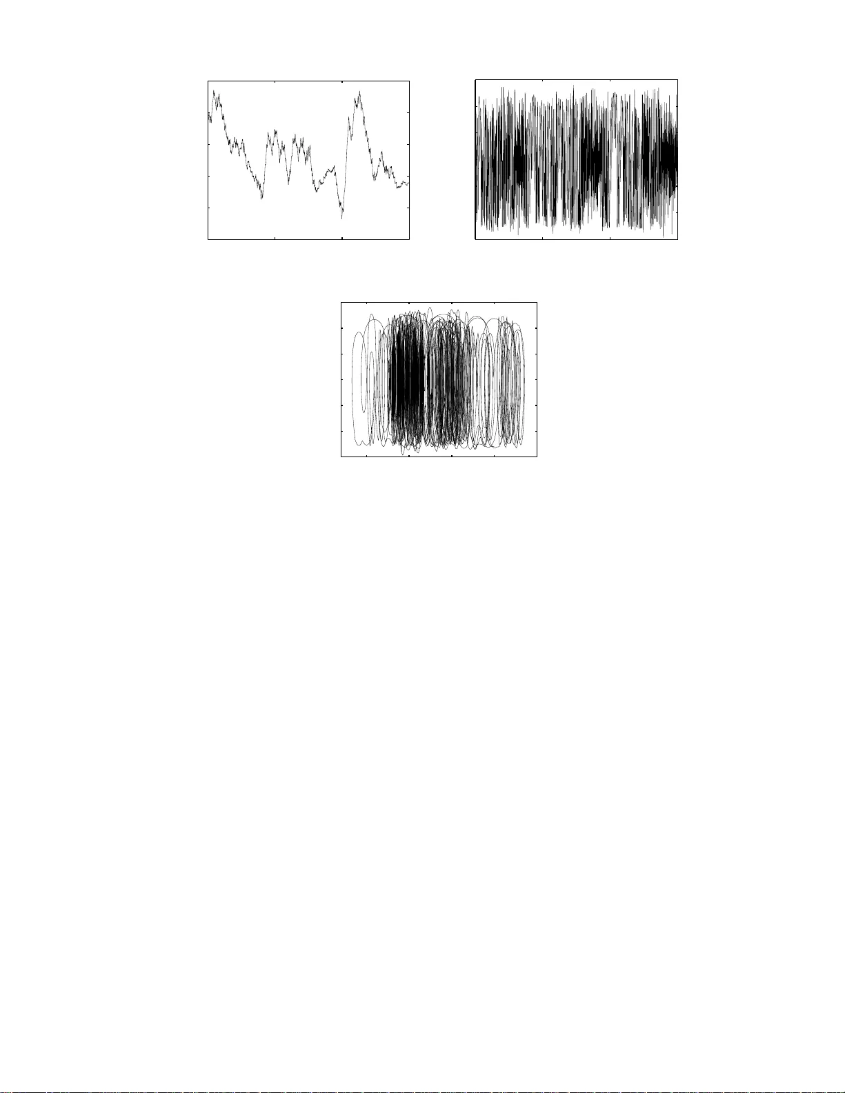
Univ ersal functions and exactly solv a ble cha otic systems M´ onica A. Garc ´ ıa- ˜ Nustes ∗ and Jorg e A. Gonz´ alez Centr o de F ´ ısic a, Instituto V enezolano de I nvestigaciones Cient ´ ıfic as, Ap artado 21827, Car ac as 1020-A, V enezuela Emilio Hern´ andez-Gar c ´ ıa Dep artament o de F ´ ısic a Inter disciplinar,Instituto Me diterrne o de Estudios Avanz ados CSIC-Universidad de las Islas Bale ar es, E-07122-Palma de Mal lor c a, Esp a˜ na A universa l differential equ ation is a nontrivial differenti al equation the sol utions of which ap- proximate to arbitrary accuracy an y contin uous function on any interv al of the real line. On the other hand, th ere has been muc h interest in exactly solv able chaotic maps. An important problem is to generalize th ese results to continuous systems. Theoretical analysis w ould allow us to p ro ve theorems about these systems and predict new phenomena. In the p resen t paper we discuss the concept of universal functions and their relev ance to th e theory of universal differential equ ations. W e p resen t a conn ection b etw een universal functions and solutions to chaotic systems. W e will sho w the statistical indep end ence b etw een X ( t ) and X ( t + τ ) (when τ is not equal to zero) and X ( t ) is a solution to some chaoti c systems. W e wil l construct universal functions that b eha ve as delta-correlated noise . W e wil l construct universa l dynamical systems with truly noisy solutions. W e will discuss physicall y realizable dyn amical systems with universal-lik e prop erties. I. INTRO DUCT ION Recently there has b een great interest in exactly solv a ble chaotic systems [1, 2, 3, 4 , 5, 6, 7]. S. Ulam and J. von Neumann were the first to prov e that the gener a l solution to the lo g istic map can b e found [1, 2]. It is very impo rtant to e xtend these res ults to contin uous systems. Theor etical ana ly sis would allow us to pr ov e theorems ab out these systems and predict ne w phenomena. Another surprising pa rallel development is that of “universal differential equations” . A universal differen tial equation is a nontrivial different ial- algebraic equation with the pro per t y that its solutions approximate to arbitrary accuracy any c o nt inuous function on any interv al of the r eal line [8, 9, 10, 11, 12, 13, 14, 15, 16]. Rub el found the first known universal differen tial equation b y showing that there are differen tial equations o f low order (e.g. fourth-order ) whic h ha ve solutions arbitra rily close to a n y prescrib e d function [8]. The existence of universal different ial equations illustr ate the amazing co mplexit y that solutio ns of lo w-or der dynamical systems can hav e. In the present pape r, we will review some development s in the ar eas of universal differential equations and exactly so lv able chaotic dynamical systems. W e will discuss the concept o f “univ ers al functions ” and their relev ance to the theo ry of universal differential equations. W e will sho w the sta tistical independence b et ween X ( t ) and X ( t + τ ) (when τ 6 = 0) a nd X ( t ) is the so lution to some chaotic dynamical systems. W e will pr esent a connection b et ween univ ersa l functions and solutions to c hao tic systems. W e will constr uct univ ersa l functions that behave as δ - correlated noise. W e will construct universal differ en tial equations with truly noisy solutio ns. W e will discuss physically realizable dynamical systems with universal prop erties and their p otential applications in secure communications and ana log computing. II. UNIVERSAL DIFFERENTIAL EQUA T IONS Rubel’s theorem [8] is: There ex is ts a nontrivial fo ur th- order differen tial equation P ( y ′ , y ′′ , y ′′′ , y ′′′′ ) = 0 , (1) where y ′ = dy dt , P is polynomia l in four v a riables, with integer co efficients, s uc h tha t for any contin uo us function φ ( t ) on ( −∞ , ∞ ) and for a n y p ositive contin uous function ε ( t ) on ( −∞ , ∞ ), there exists a C ∞ solution y ( t ) such that | y ( t ) − φ ( t ) | < ε ( t ) for all t on ( −∞ , ∞ ). A pa r ticular ex ample of Eq.(1) is the following: 3 y ′ 4 y ′′ y ′′′′ 2 − 4 y ′ 4 y ′′′ 2 y ′′′′ + 6 y ′ 3 y ′′ 2 y ′′′ y ′′′′ + 24 y ′ 2 y ′′ 4 y ′′′′ − 29 y ′ 2 y ′′ 2 y ′′′ 2 − 12 y ′ 3 y ′′ y ′′′ 3 + 12 y ′′ 7 = 0 , (2) ∗ Corresp onding author. F ax: +58-212-5041566 ; e-mai l: mogarcia@ivic.ve 2 (a) (b) FIG. 1 : Solution y ( t ) for (a) e q uation (3), and (b) equation (4) with m = 4. Duffin [10] has found t wo additional families o f universal differential equations: my ′ 2 y ′′′′ + (2 − 3 m ) y ′ y ′′ y ′′′ + 2( m − 1) y ′′ 3 = 0 (3) and m 2 y ′ 2 y ′′′′ + 3 m (1 − m ) y ′ y ′′ y ′′′ + (2 m 2 − 3 m + 1 ) y ′′ 3 = 0 (4) where m > 3. Recently , Brig gs [17] has found a new family: y ′ 2 y ′′′′ − 3 y ′ y ′′ y ′′′ + 2(1 − n − 2 ) y ′′ 3 = 0 , (5) for n > 3. The s olutions a r e C n . W e w ould lik e to make some o bserv a tions ab out these equations. Rubel’s function y ( t ) in E q.(2) is C ∞ but not rea l-analytic, typically having a co un table num b er of es sent ial singularities. The functions used to reco nstruct the so lutions to Eq.(2) a re of the form y = Af ( αt + β ) + B , (6) where f ( t ) = R g ( t ) dt , g ( t ) = exp h − 1 (1 − t 2 ) i for − 1 < t < 1, with g ( t ) = 0 for all other t . The s olutions to equations (3) are trig onometric splines. The kernel g ( t ) is defined as g ( t ) = a [cos bt + c ] m . (7) On the other hand, the k ernel emplo yed to obtain the solutions to Eq. (4) are p olynomial splines: g ( t ) = a [1 − ( bt + c ) 2 ] m . (8) The s olutions a r e very unstable. This phenomenon can b e o bserved in Fig.(1a) a nd Fig.(1 b). II I. EXACTL Y SOL V ABLE CHAOTIC MAPS Ulam a nd von Neumann [1, 2] pr ov ed tha t the function X n = sin 2 ( θπ 2 n ) is the general solution to the logistic map X n +1 = 4 X n (1 − X n ) . (9) Recently , many pap er s hav e b een dedicated to exactly solv able chaotic maps [3, 4, 5, 6, 7, 1 8, 19, 20, 21]. In some of these pap ers, the author s not only find the explicit functions X n that solve the maps, but a ls o they discuss 3 the s tatistical pro per ties of the sequence s generated by the chaotic maps. F or many of the maps discussed in the men tioned pap ers, the exact solution can be written a s X n = P ( θk n ) , (10) where P ( t ) is a perio dic function, θ is a fix ed r eal parameter and k is an integer. F or instance, X n = co s(2 π θ 3 n ) is the so lution to map X n +1 = X n (4 X n 2 − 3). This is a particula r case of the Chebyshev maps [5]. V ery in teresting c haotic maps of type X n +1 = f ( X n ) can be constructed when function P ( t ) is a combination of trigonometric , e lliptic and other gener alized p erio dic functions [6]. IV. ST A TISTICAL INDEPENDENCE W e will consider statis tica l indep endence in the sense o f M. Kac [22, 23, 24, 25]. In this fra mew or k, t wo functions f 1 ( t ) , f 2 ( t ) are indepe ndent if the prop ortion of time during which, simultaneously , f 1 ( t ) < α 1 and f 2 ( t ) < α 2 is e qual to the pro duct o f the prop ortions of time during whic h separately f 1 ( t ) < α 1 , f 2 ( t ) < α 2 . First, w e will present some r esults ab out functions of natural arg umen t n . Consider a genera liz ation to the functions that are exac t solutions to the Cheb yshev maps: X n = cos(2 π θ Z n ) , (11) where Z is a generic real num b er. An y set of subsequences X s , X s +1 , · · · , X s + r (for any r ) c o nstitutes a s et o f statistically indep e nden t random v ar ia bles. If E ( X ) is the exp ected v a lue o f quantit y X , let us define the r - o rder cor r elations [18]: E ( X n 1 X n 2 · · · X n r ) = 1 Z − 1 dX 0 [ ρ ( X 0 ) X n 1 X n 2 · · · X n r ] . (12) Here E ( X n ) = 0 , − 1 6 X n 6 1, ρ ( X ) = 1 π √ 1 − X 2 , X 0 = cos(2 π θ ). In Ref. [27] it is shown that E ( X n 0 s X n 1 s +1 · · · X n r s + r ) = E ( X n 0 s ) E ( X n 1 s +1 ) · · · E ( X n r s + r ) (13) for a ll pos itiv e int ege r s n 0 , n 1 , n 2 , · · · , n r . The results abo ut the indep endence of subseque nc e s of function X n = cos(2 π θ Z n ) can be extended to more ge neral functions a s the following: X n = P ( θ T Z n ) , (14) where P ( t ) is a perio dic function, T is the p erio d of P ( t ) and θ is a parameter [27]. M. Kac [22, 23, 24, 25] has s tudied indep endence of differ en t contin uous functions, e.g. f 1 ( t ) = c os ( t ) , f 2 ( t ) = cos ( √ 2 t ). How ever, these functions are perio dic [22, 23, 24, 25, 26]. W e are interested in the indep endence of contin uous functions in the sense that the s ame function can pro duce statistically indep enden t random v ar iables if ev aluated at different times. That is, the functions f ( t ) and f ( t + τ ) should b e statistically indep endent if τ 6 = 0. Periodic functions will nev er poss ess this proper t y . Using the theor ems of Refs. [22, 25], we obtain the result that functions f 1 = cos( λ 1 t ) , f 2 = cos( λ 2 t ) , · · · , f r = cos( λ r t ) constitute a set of independent functions when the num b ers λ 1 , λ 2 , · · · , λ r are linear ly indep endent ov er the rationals. This is equiv a len t to the fa ct that if α 1 , α 2 , · · · , α r are ra tio nal, α 1 λ 1 + α 2 λ 2 + · · · + α r λ r = 0 o nly if α 1 , α 2 , · · · , α r are all zero. Consider the following contin uo us function constructed as a contin uous analogous to the function (11): X ( t ) = cos ( θ e bt ) . (15) It is not difficult to s ee that the functions X ( t ) and Y ( t ) = X ( t + τ ) are indep endent (in M. Kac’s s ense) for (Lebe s gue) a lmost all τ > 0. Note that Y ( s ) = c os λs, X ( s ) = cos s , where s = θ e bt , λ = e bτ . The pro of of the fact that Y ( s ) = co s( λs ) and X ( s ) = cos s are indep endent is tr ivial based on the theorems of M. Kac[22, 2 3, 24, 25]. 4 V. ALGEBRAIC DIFFERENTIAL EQUA TIONS AND CHAOTIC SOLUTIONS There ex is ts a nontrivial fo ur th- order differen tial equations of t yp e: P ( y ′ , y ′′ , y ′′′ , y ′′′′ ) = 0 , (16) where P is a p o lynomial in four v ar iables, w ith int eger co efficients, such tha t there exist solutions y ( t ) with the prop erty that y ( t ) and y ( t + τ ) are sta tistically indep endent functions for mo st τ . A par ticular example of Eq .(1 6) is the following: 2 y ′ y ′′ − 3 y ′ y ′′′ + y ′ y ′′′′ − y ′′ y ′′′ + ( y ′′ ) 2 = 0 . (17) The function y ( t ) = cos ( e t ) is a s olution to this equatio n. Here we should make a remark. The differential equations (2), (3), (4 ), (5), a nd (17) a re similar in the sense that they a re all of the t yp e (1) or (16), and that all the terms are nonlinear . W e hav e shown that the equation (1 7) p ossesses en tire solutio ns as the fo llowing y ( t ) = co s( e t ) which ha s the prop erty that y ( t ) and y ( t + τ ) are not corr elated. This so lution is rea l-analytic on ( −∞ , ∞ ). This result shows that equations of t yp e (16) can generate hig h complexity . VI. UNIVERSAL FUNCT IONS In this sectio n we will follow the appro ach to universal equations develop ed by R. C. Buck [9] and M. Boshernitzan [13]. In this pap er, a family o f functions will b e ca lled universal if these functions ar e dense in the spac e C [ I ] of all cont inuous real functions o n the in terv al I ⊂ R . R. C. Buc k has obtained universal par tial algebraic differ e n tial equations using a very deep metho d: Kolmo gorov’s solution of Hilber t’s Thirteen Problem. He has found that solutions to a smo oth PDE can b e dense in C [ I ][9]. The adv antage of this approa ch is that we ca n c o nstruct universal functions which a re real- analytic on R = ( −∞ , ∞ ). Thu s, the cor resp onding universal equations will hav e so lutio ns that are r e a l- analytic on R = ( −∞ , ∞ ). F or an y interv al I ⊂ R = ( −∞ , ∞ ), C [ I ] denotes the Banach space of re a l- v alued cont inuous bo unded functions on I . Boshernitzan [1 3] has studied the following families of functions: y ( t ) = t + a Z 0 bd 1 + d 2 − cos( bs ) cos( e s ) ds + c, (18) where d > 0, a , b , and c are r eal par a meters. Another imp ortant family of functions is defined as follows: y ( t ) = b n t + a Z 0 cos 2 n 2 ( bs ) cos( e s ) ds + c, (19) where a , b , c are pa r ameters and n ≥ 1 is an in teger constant. W e should stress that a ll the functions in the family given by E q.(19) ar e r eal-analytic on R = ( −∞ , ∞ ) and ent ire. Boshernitzan has pr oved that each of the families o f functions, (18) and (19), is dense in C [ I ], for a ny compact int erv al I = [ a, b ] ⊂ R . So these functions a re univ ersal. Hence it is pos sible to construct universal systems using these universal families of functions. Other re sults o f Boshernitzan ar e the following. There exists a nontrivial six th- order alge br aic differential equa tion of the form P ( y ′ , y ′′ , · · · , y (6) ) = 0 , (20) such that any functions in the family (18) is a solution. And there exis ts a nontrivial seven th- or der algebraic differen tial equation o f the form P ( y ′ , y ′′ , · · · , y (7) ) = 0 , (21) 5 0 10 30 50 −2 −1 0 1 2 t y(t) FIG. 2 : Time- series generated by (19). such tha t any function in the family (19) is a solution. F rom these theor e ms one can obtain an imp ortant results for us: There exists a nontrivial seven th- orde r differential equation, the r eal- analytic e ntire solutions of which are dense in C [ I ], for any compact interv al I ⊂ R . Thus this equation is universal. Boshernitza n has not constructed this equation explicitly . The p os sibilit y of an en tire approximation for any dynamics is v ery promising for practical a pplications. VII. UNIVERSAL SYSTEMS OF DIFF ERENTIAL EQUA TIONS Using the inverse problem tec hniques and theorems of the w orks[8, 9, 10, 11, 1 2, 13, 14, 15, 16], and the results contained in the pr esent pap er, it is p ossible to write down a system of differen tial equations suc h that a n y function of the family (19 ) is a solution: P 1 [ x, x ′ , · · · , x ′′′ ] = 0 , (22) P 2 [ y , y ′ , · · · , y ′′′ ] = 0 , (23) z ′ = A x y . (24) Eq. (2 2) is constructed in such a w ay that a ll the functions x = a [cos( bx + c )] m are so lutions. The sp ecific p olyno mial P 1 is P 1 = mx ′′′ x 2 − (3 m − 2) x ′′ x ′ x + (2 m − 2) x ′ 3 , (25) where m = 2 n 2 > 2. Eq.(23) is constructed in such a w ay tha t y ( t ) = cos( e t ) is a s olution. The sp ecific p olynomial P 2 is defined as P 2 = y y ′′′ − 3 y y ′′ − y ′ y ′′ + y ′ 2 + 2 y ′ y . (26) The vector solution ( x, y , z ) to the system of equa tions (22-24) is such that for the v a r iable z ( t ) the functions (1 9) are solutions. Thu s, the system of differential eq uations (22-2 4) can gene r ate, in v ariable z ( t ), universal functions. Note tha t this is a seven th- o rder dynamical system as w as predicted by Bos he r nitzan[13]. The s ystem of equations (22- 2 4) is present ed in this paper for the first time. VII I. NOISY FUNCTIONS In this section we use several concepts and results from proba bilit y theory a nd mathematical statistics which can be consulted for instanc e in the bo o ks[28, 29]. In sections (IV) and (V) we discus s ed the function y ( t ) = cos( e t ). Note that the statistical independence b etw een functions y 1 ( t ) = co s( e t ) a nd y 2 ( t ) = co s( e t + τ ) implies the following rela tionship: E [ y k 1 1 ( t ) y k 2 2 ( t )] = E [ y k 1 1 ( t )] E [ y k 2 2 ( t )] , (27) 6 for a ll pos itiv e int ege r s k 1 and k 2 . Here E [ x ( t )] is the exp ected v a lue of quantit y x ( t ). It can b e calculated a s follows: E [ x ( t )] = lim T →∞ 1 T T Z 0 x ( t ) dt. (28) As E [ y 1 ( t )] = 0, w e obtain that E [ y ( t ) y ( t ′ )] = 0 , (29) for t 6 = t ′ . In fac t, a direct calcula tio n of the auto cor relation function c o nfirms this results: C ( τ ) = lim T →∞ 1 T T Z 0 cos( e t ) cos( e t + τ ) dt = 0 (30) for τ 6 = 0. Another imp ortant sta tistical prop erty of the indep endent functions y 1 ( t ) and y 2 ( t ) is η ( y 1 ( t ) , y 2 ( t )) = η ( y 1 ( t )) η ( y 2 ( t )) , (31) where η ( y ) is the probabilit y density . In fac t, η ( y 1 ) = 1 π p 1 − y 2 1 , (32) η ( y 2 ) = 1 π p 1 − y 2 2 , (33) η ( y 1 , y 2 ) = 1 π 2 p (1 − y 2 1 )(1 − y 2 2 ) . (34) Fig.(3) sho ws these prop erties. Let us in tro duce a g e neralized function y ( t ) = cos( φ ( t )) . (35) W e sho uld re mark here that the arg umen t of function (35), φ ( t ), do es no t need to b e exp onential all the time for t → ∞ , in o rder to g enerate no isy dynamics . In fac t, it is sufficient for function φ ( t ) to be a b ounded nonper io dic oscilla ting function whic h p oss esses rep eating int erv als with truncated exponential b ehavior[30]. A deep analysis o f the Boshernitzan’s proo fs of the fact that the families functions (18) a nd (19) are dense in C [ I ] shows that the r andom b ehavior of functions o f t yp e (35) is crucial[13]. W e are go ing to pres en t here tw o exa mples of thes e functions. The firs t is defined by the e q uation x ( t ) = c os { A exp [ a 1 sin( ω 1 t + φ 1 ) + a 2 sin( ω 2 t + φ 2 ) + a 3 sin( ω 3 t + φ 3 )] } . (36) The s econd function is given by the equa tion y ( t ) = co s { B 1 sinh [ a 1 cos( ω 1 t + φ 1 ) + a 2 cos( ω 2 t + φ 2 )] + B 2 cosh [ a 3 cos( ω 3 t + φ 3 ) + a 4 cos( ω 4 t + φ 4 )] } . (37) Note that if the frequencies ω i are linearly independent ov er the rationals, in b oth cases , the argument function φ ( t ) is a nonp erio dic function with truncated exponential b ehavior. Theoretical a nd numerical in vestigations give the res ult that, when the pa r ameters satisfy certain co nditio ns, they behave as the solutio ns to c haotic systems[20]. Figure (4 ) s hows that the time- ser ies genera ted by (36) is very co mplex. 7 −1 0 1 0 1000 y 1 (t) η (y 1 (t)) −1 0 1 0 1500 y 2 (t) η (y 2 (t)) (a) y 2 (t) (b) FIG. 3 : (a) Proba bility density η ( y 1 ) a nd η ( y 2 ) , (b) P robability density η ( y 1 , y 2 ). FIG. 4 : Time- ser ies generated b y function (37). F urthermor e, they b ehav e in such a wa y that y 1 = y ( t ) and y 2 = y ( t + τ ) are statistica lly indep endent functions (in M. K ac’s sense) for τ 6 = 0. An illus tr ation of these pro per ties is that η ( y 1 , y 2 ) = η ( y 1 ) η ( y 2 ) . (38) Other no isy functions can b e obtained using another g e ne r alization x ( t ) = P [ φ ( t )] , (39) 8 where P ( y ) is a general p erio dic function, and φ ( t ) is a nonp erio dic expo ne ntial-like function a s b efore. The pr obability density o f these functions dep ends on the c hoice of P ( y ). An imp orta nt example is the following x ( t ) = ln  tan 2 [ φ ( t )]  . (40) The pr obability density o f the time- series pro duced by function (40 ) is a Gaussia n-like law[30]. Another re ma rk able prop erty of function (4 0) is the following: E [ x ( t ) x ( t ′ )] = D δ ( t − t ′ ) , (41) where E [ x ( t ) x ( t ′ )] is defined as in E q.(27), and δ ( t − t ′ ) is Dirac’s delta- function. Thu s, function (40) po ssesses all the pr op erties usually requir ed in the s tochastic equa tions with δ - correla ted nois y per turbations[31, 32]. IX. PR OPER TIES OF CHA OTIC SOLUTIONS A Lyapuno v exp onent of a dynamica l sy stem characterizes the rate of separa tio n of infinitesimally clo se tra jectories. Suppo se δ z 0 is the initial distance betw een tw o tra jectories, and δ z ( t ) is the distance b etw een the tra jecto ries at time t . The ma ximal Lyapunov exp onent can b e defined a s follows: λ = lim t →∞ 1 t ln     δ z ( t ) δ z 0     . (42) Consider the dynamical system d~ x dt = ~ F ( ~ x ) . (43) The v aria tional equation is d ~ φ dt = D x ~ F ( ~ x ) ~ φ ( t ) . (44) The L yapunov e x po ne nt λ satisfies the equation λ = lim t →∞ 1 t ln | φ ( t, x 0 ) | . (45) A so lution will be considered chaotic if λ > 0. A r elated prop erty of c haotic systems is s ensitive dep endence on initial conditions[33, 34]. F unction y ( t ) = cos[exp( t + φ )] (46) has b een shown to b e the solution to some dynamical sy stem. Her e φ can define the initial c ondition. The L yapunov e x po ne nt of solution (46) can b e calculated exactly λ = ln e = 1 > 0. The functions (36), (37), a nd (40) are a lso c hao tic solutions in this sense. The initial conditions a r e defined by the parameters φ 1 , φ 2 and φ 3 . Let us discuss sens itiv e dependence on initial conditions in the context of these functions. Let S b e the set of functions defined by one of the families g iven by equations (36), (37), (40), a nd (46). A set S exhibits sensitive dep endence if ther e is a δ such that for any ǫ > 0 and e ach y 1 ( φ, t ) in S , there is a y 2 ( φ ′ , t ), also in S , such that | y 1 ( φ, 0) − y 2 ( φ ′ , 0) | < ǫ , and | y 1 ( φ, t ) − y 2 ( φ ′ , t ) | > δ for so me t > 0. The e xpo nen tial behavior in the arguments o f these functions ((36), (37), (40), and (4 6)) ma kes them chaotic (see a discuss ion in Ref. [35]). All these functions poss ess equiv a len t dy namical and statistical prope r ties. F ollowing Bosher nitzan theory [13] of mo dulo 1 sequences , it is p ossible to construct the following families o f universal functions: y ( t ) = bn t + a Z 0 cos 2 n 2 ( bs ) x ( s ) ds + c, (47) where x ( s ) is o ne of the functions ((36), (37 ),(40)). 9 X. DYNAMICAL SY STEMS WITH NOISY SOLUTIONS In this s ection we will construct autonomous dynamical systems, the solutions of which are the nois y functions discussed in the previous section. Consider the following dynamical sy stem x ′ 1 = x 1 [1 − ( x 2 1 + y 2 1 )] − ω 1 y 1 , (48) y ′ 1 = y 1 [1 − ( x 2 1 + y 2 1 )] + ω 1 x 1 , (49) x ′ 2 = x 2 [1 − ( x 2 2 + y 2 2 )] − ω 2 y 2 , (50) y ′ 2 = y 2 [1 − ( x 2 2 + y 2 2 )] + ω 2 x 2 , (51) x ′ 3 = x 3 [1 − ( x 2 3 + y 2 3 )] − ω 3 y 3 , (52) y ′ 3 = y 3 [1 − ( x 2 3 + y 2 3 )] + ω 3 x 3 , (53) z ′ = [ a 1 x 1 + a 2 x 2 + a 3 x 3 ] z , (54) u ′ = A c o s[ θ z ] . (55) Note that the equatio ns (48-53) define three pa ir s of limit-cyc le tw o-dimensiona l dynamical systems. The exact solutions to these limit-cycle sys tems are well-known. If we define Q ( t ) = a 1 x 1 ( t ) + a 2 x 2 ( t ) + a 3 x 3 ( t ) , (56) the function Q ( t ) will b e a quasip erio dic time- series. Equation (5 4) will provide us with the appro priate nonp erio dic tr uncated exp onent ial behavior. Finally , the solutio n to equation (55) will have pr ope rties eq uiv alent to these of function (36). The so lution to E q .(55) is chaotic in the sense discussed in section (IX). The maximal Lyapunov exp o nent of this dynamical system is positive and the so lutions po ssess sensitiv e de p endence on initial conditions. If we need more v aria bility in the solutions, w e can cons truct a dynamical system such that the r ig ht - hand par ts of the equations dep end on function u ( t ) whic h is known to b e highly nonperio dic. These ideas lead to the next autonomo us dynamical s y stem: x ′ 1 = x 1 [1 − ( x 2 1 + y 2 1 )] − ω 1 y 1 + ε 1 u, (57) y ′ 1 = y 1 [1 − ( x 2 1 + y 2 1 )] + ω 1 x 1 , (58) x ′ 2 = x 2 [1 − ( x 2 2 + y 2 2 )] − ω 2 y 2 + ε 2 u, (59) y ′ 2 = y 2 [1 − ( x 2 2 + y 2 2 )] + ω 2 x 2 , (60) x ′ 3 = x 3 [1 − ( x 2 3 + y 2 3 )] − ω 3 y 3 + ε 3 u, (61) y ′ 3 = y 3 [1 − ( x 2 3 + y 2 3 )] + ω 3 x 3 , (62) z ′ = [ a 1 x 1 + a 2 x 2 + a 3 x 3 + a 4 u ] z , (63) u ′ = A 1 cos[ θ 1 z ] + A 2 cos[ θ 2 z ] . (64) Now a ll the compo ne nts of the so lutions to system (57-6 4) are chaotic. The solution to E q.(64) is chaotic in the sense that the maximal Lyapuno v exp onent is positive (see section (IX)). In the dynamica l sy stem (57-6 4), the limit cycle subsystems (5 7,58), (59,60) and (61,62) are now coupled to the chaotic comp onent u ( t ). W e now address the function (37). W e ha ve to c o nstruct a dynamical system with so lutions that b ehav e like this function. 10 0 200 400 600 −1 −0.5 0 0.5 1 1.5 u(t) t (a) 0 200 −0.1 −0.05 0 0.05 0.1 0.15 u’(t) t (b) −0.5 0 0.5 1 1.5 −0.1 0 0.1 0.15 u’(t) u(t) (c) FIG. 5: ( a)Time- series o f v ariable u ( t ),(b) u ′ ( t ) and, (c) P hase por trait generated by the autonomous dynamical system (57-6 4). Consider the autonomo us dynamical sy stem: x ′ 1 = x 1 [1 − ( x 2 1 + y 2 1 )] − ω 1 y 1 , (65) y ′ 1 = y 1 [1 − ( x 2 1 + y 2 1 )] + ω 1 x 1 , (66) x ′ 2 = x 2 [1 − ( x 2 2 + y 2 2 )] − ω 2 y 2 , (67) y ′ 2 = y 2 [1 − ( x 2 2 + y 2 2 )] + ω 2 x 2 , (68) x ′ 3 = x 3 [1 − ( x 2 3 + y 2 3 )] − ω 3 y 3 , (69) y ′ 3 = y 3 [1 − ( x 2 3 + y 2 3 )] + ω 3 x 3 , (70) x ′ 4 = x 4 [1 − ( x 2 4 + y 2 4 )] − ω 4 y 4 , (71) y ′ 4 = y 4 [1 − ( x 2 4 + y 2 4 )] + ω 4 x 4 , (72) z ′ 1 = − ( a 1 ω 1 y 1 + a 2 ω 2 y 2 ) z 2 , (73) z ′ 2 = − ( a 1 ω 1 y 1 + a 2 ω 2 y 2 ) z 1 , (74) z ′ 3 = − ( a 3 ω 3 y 3 + a 4 ω 4 y 4 ) z 4 , (75) z ′ 4 = − ( a 3 ω 3 y 3 + a 4 ω 4 y 4 ) z 3 , (76) u ′ = A c o s[ B 1 z 1 + B 4 z 4 ] . ( 77 ) The e xplanation of this sy s tem is similar to that of equations (48-55). 11 XI. UNIVERSAL FUNCT IONS A ND DYNAMICAL SYSTEMS Based on the prop erties o f functions (15), (18), (19), (36), and (37), we pro p os e the following set o f equations as a universal dynamical sys tem: x ′ 1 = x 1 [1 − ( x 2 1 + y 2 1 )] − ω 1 y 1 , ( 78 ) y ′ 1 = y 1 [1 − ( x 2 1 + y 2 1 )] + ω 1 x 1 , ( 79 ) x ′ 2 = x 2 [1 − ( x 2 2 + y 2 2 )] − ω 2 y 2 , ( 80 ) y ′ 2 = y 2 [1 − ( x 2 2 + y 2 2 )] + ω 2 x 2 , ( 81 ) x ′ 3 = x 3 [1 − ( x 2 3 + y 2 3 )] − ω 3 y 3 , ( 82 ) y ′ 3 = y 3 [1 − ( x 2 3 + y 2 3 )] + ω 3 x 3 , ( 83 ) x ′ 4 = x 4 [1 − ( x 2 4 + y 2 4 )] − ω 4 y 4 , ( 84 ) y ′ 4 = y 4 [1 − ( x 2 4 + y 2 4 )] + ω 4 x 4 , ( 85 ) z ′ 1 = − ( a 1 ω 1 y 1 + a 2 ω 2 y 2 ) z 2 , (86) z ′ 2 = − ( a 1 ω 1 y 1 + a 2 ω 2 y 2 ) z 1 , (87) z ′ 3 = − ( a 3 ω 3 y 3 + a 4 ω 4 y 4 ) z 4 , (88) z ′ 4 = − ( a 3 ω 3 y 3 + a 4 ω 4 y 4 ) z 3 , (89) u ′ = ω 1 nx 2 n 2 1 cos [ B 1 z 1 + B 4 z 4 + a ] . (90) The solution to Eq.(9 0) is a function with all the proper ties of Bo shernitzan’s family of functions (19). Th us this family of functions is dense in C [ I ]. The dynamical sys tem (78-90) has b een constr ucted using the same technique developed in the pap ers [9, 1 3] a bo ut universal differential equa tio ns. That is, a family of functions known to b e dense in C [ I ] is utilized as the sta rting po in t for a n inv erse-pr oblem pro cedure that cons is ts in reconstructing differential equa tions the solutions o f which are the functions that belong to the univ ersa l family o f functions. This dynamical system can b e r ealized in practice using nonlinear c ir cuits as discussed in Ref.[21]. XII. CONCLUSIONS W e ha ve discussed the concept of “Univ ersal functions” and their relev ance to the theor y of universal differential equations. W e b elieve that the metho d of constructio n o f universal differ en tial equa tions using universal functions is mor e powerful that the metho d bas ed on s plines. W e hav e found a co nnection b etw een the universal families of functions prop osed in a very impo rtant paper by Boshernitzan [1 3] and recently o bta ined exa ct solutions to chaotic systems. W e hav e shown that some functions x ( t ) tha t ar e exact s o lutions to chaotic systems p oss ess the prop erty that y 1 = x ( t ) and y 2 = x ( t + τ ) are statistically indep endent functions in the sense o f M. Kac. W e hav e co nstructed alg e br aic differential e q uations that p osses s solutions w ith these prop erties. Thes e eq uations hav e, in fa ct, so lutions that behave lik e noise. Some kno wn univ ersal eq ua tions can only approximate these functions using “solutions ” constructed with p olyno- mial or trigonometric s plines. The actual exact solutions to the differen tial equations ar e not “ noisy”. W e hav e co ns tructed a system of differential equations, the so lutions of which are Boshernitza n’s functions. Bosher - nitzan’s functions a re rea l a nalytic o n R = ( −∞ , ∞ ). One of the families of Boshernitza n’s functions are r eal- analytic ent ire functions o n R = ( −∞ , ∞ ). W e ha ve developed univ ersa l- lik e functions that behave as δ - cor related noise. W e have constructed physically re a lizable dynamical systems that p oss e s s so lutions that are universal-like functions. The theor y of universal differential equa tions has b een linked from the b eginning with applications in ana lo g computing[8, 1 0, 11, 12, 13, 15, 16]. W e b elieve that the prese nt results ca n b e of interest in the construction of rea l analo g computer s beca use the discussed dyna mical sys tems can b e realized in practice using nonlinear circuits[21, 30, 35]. 12 They can also find applications in chaos- based secur e communications technologies [21, 2 7]. [1] S. M. Ulam, J. von Neumann, Bul l. A m. M ath. So c. 53 , 1120 (1947) [2] P . S tein, S. M. U lam, R ozpr awy Matematyczne 39 , 401 (1984) [3] T. Geisel, V. F airen, Phys. L ett. A105 , 263 (1984) [4] S. Katsura, W. F uk uda, Physic a A130 , 597 (1985) [5] S. Kaw amoto, T. Tsubata, J. Phys. So c. Jap an 65 , 3078 (1996) [6] K. Umeno, Phys. Re v. E55 , 5280 (1997) [7] T. Kohda, H. F ujisaki, Physic a D148 , 242 (2001) [8] L. A. Rub el, Bul l . A m. Math. So c. (New Series) 4 , 345 (1981) [9] R. C. Buck, J. Di ff. Equations 41 , 239 (1981) [10] R. J. Duffin, Pr o c. Natl. A c ad. Sci. USA 78 , 4661 (1981 ) [11] L. A. Rub el, T r ans. A m. Math. So c. 280 , 43 (1983) [12] M. Boshernitzan, L. A. R ub el Analysis 4 , 339 (1985) [13] M. Boshernitzan, Ann. Math. 124 , 273 (1986) [14] C. Elsner, Math. Nachr. 157 , 235 (1992) [15] L. A. Rub el, Il l inois J. Math 36 , 659 (1992) [16] L. A. Rub el, J. Appr ox. The ory 84 , 123 (1996) [17] K. Briggs, A nother Universal Differ ential Equation Arxiv:math.CA/0211142v1 (2002) [18] C. Bec k, Nonline arity 4 , 1131 (1991) [19] H. N. Nazareno, J. A. Gonz´ alez, I. F. Costa, Phys. R ev. B57 , 13583 (1998) [20] J. A. Gonz´ alez, L. I. Reyes, L. E. Guerrero, Chaos 11 , 1 (2001) [21] J.A. Gonz´ alez, L.I. Reyes, J.J. Su´ arez, L. E. Guerrero, G. Guti´ errez, Phys. L ett. A 295 , 25 (2002) [22] M. Kac, Stud. Mathematic a 6 , 46 (1936 ) [23] M. Kac, H. Steinhaus, Stud. Mathematic a 6 , 59 (1936) [24] M. Kac, H. Steinhaus, Stud. Mathematic a 6 , 89 (1936) [25] M. Kac, H. Steinhaus, Stud. Mathematic a 7 , 1 (1937) [26] M. Kac, Enigmas of Chanc e: an Auto bio gr aphy , Harp er and Row , New Y ork (1985) [27] J. A. Gonz´ alez, L. T ru jillo, J. Phys. So c. Jap an 75 , 023002 (2006) [28] P . Billingsley , Pr ob ability and Me asur e , Wiley , New Y ork (1968) [29] M. Denker, W. A. W oyczysnki, I ntr o ductory Statist ics and R andom Phenomena , Birkhauser, Boston (1998) [30] J. A. Gonz´ alez, L. I. Reyes, J. J. Su´ arez, L. E. Guerrero, G. Guti´ errez, Physic a D178 , 26 ( 2003) [31] P . H anggi, P . T alkner, M. Borko vec, R ev. Mo d. Phys. 62 , 251 (1990). [32] L. Gammaitoni, P . Hanggi, P . Jung, F. Marc hesoni, R ev. Mo d. Phys. 70 , 223 (1998). [33] J. Guckenheimer, P . H olmes, Nonline ar oscil lations, dynamic al systems, and bifur c ations of ve ctor fields , Sp ringer, N ew Y ork (1983). [34] E. Atlee Jackson, Persp e ctives in nonl i ne ar dynamics , Cambridge Universit y Press, New Y ork (1992). [35] J. J. S u´ arez, I. Rond´ on, L. T rujillo, J. A. Gonz´ alez, Chaos, Solitons and F r actals 21 , 603 (2004).