Travelling wave solutions of BBM-like equations by means of factorization

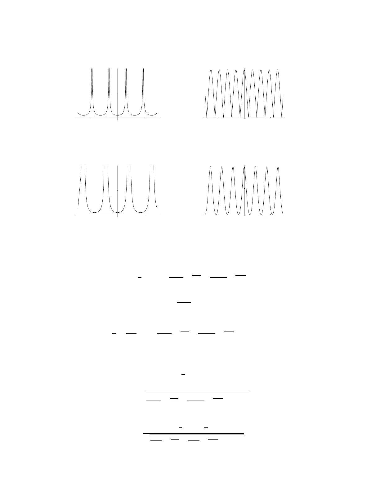
T ra velling wa ve solutions of BBM-like equation s by means of factorization S ¸ . Kuru Department of Physics, F aculty of Science, Ankara University , 06100 Ankara, T urke y Abstract In this work, we apply the factorization technique to the Benjamin-Bona-Mah ony like equations in order to get travelling wav e solutions. W e will focus on some special cases for which m 6 = n , and we will obtain these solutions in terms of W eierstrass functions. Email: kuru@science.ankara.edu.tr 1 Introd uction In this paper, we will consider the Benjamin-Bon a-Mahony (BBM) [1] like equation ( B ( m, n ) ) with a fully nonlinear dispersive term of the form u t + u x + a ( u m ) x − ( u n ) xxt = 0 , m, n > 1 , m 6 = n . (1) This equatio n is similar to the non linear dispersiv e equation K ( m, n ) , u t + ( u m ) x + ( u n ) xxx = 0 , m > 0 , 1 < n ≤ 3 (2) which has been studied in de tail by P . Rosenau and J.M. Hyman [2]. In th e literatur e there are many studies dealing with th e tra velling w av e solutions of the K ( m, n ) and B ( m, n ) equations, but in gen eral they are restricted to th e case m = n [2, 3 , 4, 5 , 6, 7, 8, 9, 10, 11, 12, 1 3, 14]. When m 6 = n , th e solutio ns of K ( m, n ) were inv estigated in [2, 3]. Our aim her e is just to search fo r solutions of the equatio ns B ( m, n ) , with m 6 = n , by means of the factorization method. W e remark that this method [15, 16, 17, 18], when it is app licable, allo ws to get directly and systematically a wide set o f solutions, comp ared with other method s used in the BBM equ ations. For examp le, th e d irect integral method used by C. Liu [19] can o nly be applied to the B (2 , 1) equation . Howe ver , the factor ization technique can be u sed to m ore equation s than the direct integral m ethod an d also, in some cases, it gives rise to m ore gen eral solution s than the sine- cosine and the tanh meth ods [11, 12, 2 0]. This factoriza tion app roach to find travelling wav e so lutions of non linear equatio ns has b een extend ed to thir d or der no nlinear ordin ary differential equations (ODE’ s) by D-S. W ang and H. Li [2 1]. When we loo k for the tra velling w ave solutions of Eq. (1), first we reduce the form of th e B ( m, n ) equ ation to a second ord er n onlinear ODE and then, we can immediately app ly factoriza tion tec hnique. Here, we will assume m 6 = n , since the case m = n has already been examined in a previous article following this meth od [14]. This p aper is organize d as f ollows. In section 2 we introd uce factorization tech nique for a special type of the secon d order n onlinear OD E’ s. Then, we app ly straightfo rwardly the factor ization to the related second order nonlinear ODE to get travelling wa ve solutions o f B ( m, n ) eq uation in section 3. W e obtain the s olutions for these n onlinear ODE’ s and the B ( m, n ) eq uation in terms of W eierstrass fu nctions in section 4. Finally , in section 5 we will add some remark s. 1 2 F acto rization of nonli near second order ODE’ s Let us consider, the following non linear second order ODE d 2 W dθ 2 − β dW dθ + F ( W ) = 0 (3) where β is con stant an d F ( W ) is an arb itrary function of W . The factorized form of th is equ ation ca n be written as  d dθ − f 2 ( W , θ )   d dθ − f 1 ( W , θ )  W ( θ ) = 0 . (4) Here, f 1 and f 2 are unk nown f unctions that may depend explicitly on W and θ . Ex pandin g (4) and comp aring with (3), we obtain the following consistency conditions f 1 f 2 = F ( W ) W + ∂ f 1 ∂ θ , f 2 + ∂ ( W f 1 ) ∂ W = β . (5) If we solve (5) for f 1 or f 2 , it will supply us to write a comp atible first ord er ODE  d dθ − f 1 ( W , θ )  W ( θ ) = 0 (6) that p rovides a solutio n for th e no nlinear ODE (3) [15, 1 6, 17, 18]. In the ap plications of this paper f 1 and f 2 will depend only on W . 3 F acto rization of the BBM-lik e equations When Eq. ( 1) has the trav e lling wa ve solutions in the form u ( x, t ) = φ ( ξ ) , ξ = hx + wt (7) where h a nd w are real constants, substituting (7) into (1) and after integrating, we get the reduced form of Eq. (1) to the second order non linear ODE ( φ n ) ξξ − A φ − B φ m + D = 0 . (8) Notice that the constants in Eq. (8) are A = h + w h 2 w , B = a h w , D = R h 2 w (9) and R is an integration constant. Now , if we intro duce the f ollowing natur al tran sformation o f th e dep endent variable φ n ( ξ ) = W ( θ ) , ξ = θ (10) Eq. (8) becom es d 2 W dθ 2 − A W 1 n − B W m n + D = 0 . (11) Now , we can ap ply the factorizatio n tech nique to Eq. (11). Com paring Eq. ( 3) and Eq . (11), we have β = 0 and F ( W ) = − ( A W 1 n + B W m n − D ) . (12) Then, from (5) we get only one consistency condition f 2 1 + f 1 W d f 1 dW − A W 1 − n n − B W m − n n + D W − 1 = 0 (13) 2 whose solutions are f 1 ( W ) = ± 1 W r 2 n A n + 1 W n +1 n + 2 n B m + n W m + n n − 2 D W + C (14) where C is an integration constant. Th us, the first order ODE (6) takes the form dW dθ ∓ r 2 n A n + 1 W n +1 n + 2 n B m + n W m + n n − 2 D W + C = 0 . (15) In order to solve th is equation for W in a more general way , let us take W in the form W = ϕ p , p 6 = 0 , 1 , then, the first order ODE (15) is rewritten in ter ms of ϕ as ( dϕ dθ ) 2 = 2 n A p 2 ( n + 1) ϕ p ( 1 − n n )+2 + 2 n B p 2 ( m + n ) ϕ p ( m − n n )+2 − 2 D p 2 ϕ 2 − p + C p 2 ϕ 2 − 2 p . (16) If we want to gu arantee the integrability of (16), the powers o f ϕ have to be integer nu mbers between 0 an d 4 [24]. Ha ving in mind the cond itions o n n, m ( n 6 = m > 1 ) and p ( p 6 = 0 ), we have the fo llowing po ssible cases: • If C = 0 , D = 0 , we can choose p and m in the following way p = ± 2 n 1 − n with m = n + 1 2 , 3 n − 1 2 , 2 n − 1 (17) and p = ± n 1 − n with m = 2 n − 1 , 3 n − 2 . (18) It can be checked that the two choices of sign in (17) and (18) gi ve rise to the s ame solutions for Eq. (1). Therefo re, we will consider only one of them. Then, taking p = − 2 n 1 − n , Eq. (1 6) becomes ( dϕ dθ ) 2 = A ( n − 1) 2 2 n ( n + 1) + B ( n − 1 ) 2 n (3 n + 1) ϕ, m = n + 1 2 (19) ( dϕ dθ ) 2 = A ( n − 1) 2 2 n ( n + 1) + B ( n − 1) 2 n (5 n − 1) ϕ 3 , m = 3 n − 1 2 (20) ( dϕ dθ ) 2 = A ( n − 1) 2 2 n ( n + 1) + B ( n − 1) 2 n (3 n − 1 ) ϕ 4 , m = 2 n − 1 (21) and for p = − n 1 − n , ( dϕ dθ ) 2 = 2 A ( n − 1) 2 n ( n + 1) ϕ + 2 B ( n − 1 ) 2 n (3 n − 1 ) ϕ 3 , m = 2 n − 1 (22) ( dϕ dθ ) 2 = 2 A ( n − 1) 2 n ( n + 1 ) ϕ + B ( n − 1 ) 2 n (2 n − 1) ϕ 4 , m = 3 n − 2 . (23) • If C = 0 , we hav e the special ca ses, p = ± 2 , n = 2 with m = 3 , 4 . Due to the same reason in the above case, we will consider only p = 2 . Then, Eq. (16) takes the form: ( dϕ dθ ) 2 = − D 2 + A 3 ϕ + B 5 ϕ 3 , m = 3 (24) ( dϕ dθ ) 2 = − D 2 + A 3 ϕ + B 6 ϕ 4 , m = 4 . (25) 3 • If A = C = 0 , we hav e p = ± 2 with m = n 2 , 3 n 2 , 2 n . In this case, for p = 2 , Eq. (16) has the following form: ( dϕ dθ ) 2 = − D 2 ϕ 4 + B 3 ϕ 3 , m = n 2 (26) ( dϕ dθ ) 2 = − D 2 ϕ 4 + B 5 ϕ, m = 3 n 2 (27) ( dϕ dθ ) 2 = − D 2 ϕ 4 + B 6 , m = 2 n . (28) • If A = 0 , we have p = ± 1 with m = 2 n, 3 n . Here, also we will take only the case p = 1 , then, we will have the equations: ( dϕ dθ ) 2 = − 2 D ϕ + 2 3 B ϕ 3 + C ϕ 4 , m = 2 n (29) ( dϕ dθ ) 2 = − 2 D ϕ + B 2 ϕ 4 + C, m = 3 n . (30) • If A = D = 0 , we ha ve p = ± 1 2 with m = 3 n, 5 n . Thus, for p = 1 2 , Eq. (16) becomes: ( dϕ dθ ) 2 = 2 B ϕ 3 + 4 C ϕ, m = 3 n (31) ( dϕ dθ ) 2 = 4 3 B ϕ 4 + 4 C ϕ, m = 5 n . (32) 4 T ra velling wa ve solutions f or BBM-like equations In this section, we will obtain the solutions of the differential eq uations (19)-(23) in terms of W eierstrass function , ℘ ( θ ; g 2 , g 3 ) , which allow u s to get th e travelling wa ve solutions of B ( m, n ) equatio ns (1). Th e re st of eq uations ( 24)-(32) can be dealt with a similar way , but they will not be worked o ut here fo r the sake of shortness. First, we will giv e some properties of the ℘ function which will be usefu l in the follo wing [25, 26]. 4.1 Relevant pr operties of the ℘ function Let us consider a differential equa tion with a quartic polynomial  dϕ dθ  2 = P ( ϕ ) = a 0 ϕ 4 + 4 a 1 ϕ 3 + 6 a 2 ϕ 2 + 4 a 3 ϕ + a 4 . (33) The solution of this equation can be written in terms of the W eierstrass function where the inv aria nts g 2 and g 3 of (33) are g 2 = a 0 a 4 − 4 a 1 a 3 + 3 a 2 2 , g 3 = a 0 a 2 a 4 + 2 a 1 a 2 a 3 − a 3 2 − a 0 a 2 3 − a 2 1 a 4 (34) and the discriminan t is given by ∆ = g 3 2 − 27 g 2 3 . The n, the solution ϕ can be found as ϕ ( θ ) = ϕ 0 + 1 4 P ϕ ( ϕ 0 )  ℘ ( θ ; g 2 , g 3 ) − 1 24 P ϕϕ ( ϕ 0 )  − 1 (35) 4 where the subindex in P ϕ ( ϕ 0 ) denotes the deri vativ e with respect to ϕ , an d ϕ 0 is one of th e roots of the polyno mial P ( ϕ ) (33). Dependin g o f the selected roo t ϕ 0 , we will h av e a solution with a d ifferent b ehavior [14]. Here, also we want to recall some other properties of the W eierstrass functions [27]: i) The case g 2 = 1 and g 3 = 0 is called lemniscatic case ℘ ( θ ; g 2 , 0 ) = g 1 / 2 2 ℘ ( θ g 1 / 4 2 ; 1 , 0) , g 2 > 0 (36) ii) The case g 2 = − 1 and g 3 = 0 is called pseudo -lemniscatic case ℘ ( θ ; g 2 , 0 ) = | g 2 | 1 / 2 ℘ ( θ | g 2 | 1 / 4 ; − 1 , 0 ) , g 2 < 0 (37) iii) The case g 2 = 0 and g 3 = 1 is called equian harmon ic case ℘ ( θ ; g 2 , 0 ) = g 1 / 3 3 ℘ ( θ g 1 / 6 3 ; 0 , 1) , g 3 > 0 . (38) Once ob tained the solutio n W ( θ ) , tak ing into account (7), (10 ) and W = ϕ p , the solu tion of Eq. ( 1) is obtanied as u ( x, t ) = φ ( ξ ) = W 1 n ( θ ) = ϕ p n ( θ ) , θ = ξ = h x + w t. (39) 4.2 The case C = 0 , D = 0 , p = − 2 n 1 − n • m = n + 1 2 Equation (19) can be expressed as ( dϕ dθ ) 2 = P ( ϕ ) = A ( n − 1) 2 2 n ( n + 1 ) + B ( n − 1) 2 n (3 n + 1 ) ϕ (40) and from P ( ϕ ) = 0 , we get the root of this polynom ial ϕ 0 = − A (3 n + 1) 2 B ( n + 1) . (41) The in variants (3 4) a re: g 2 = g 3 = 0 , and ∆ = 0 . Therefore, having in mind ℘ ( θ ; 0 , 0 ) = 1 θ 2 , we can find the solution of (19) from (35) for ϕ 0 , gi ven by (41), ϕ ( θ ) = B 2 ( n − 1) 2 ( n + 1) θ 2 − 2 A n (3 n + 1) 2 4 B n ( n + 1) (3 n + 1) . (42) Now , the solution of Eq. (1) reads from (39) u ( x, t ) =  B 2 ( n − 1) 2 ( n + 1) ( h x + w t ) 2 − 2 A n (3 n + 1) 2 4 B n ( n + 1) (3 n + 1)  2 n − 1 . (43) • m = 3 n − 1 2 In this case, our equation to solve is (20) and the polynomial has the form P ( ϕ ) = A ( n − 1) 2 2 n ( n + 1) + B ( n − 1) 2 n (5 n − 1) ϕ 3 (44) 5 with one real r oot: ϕ 0 =  − A (5 n − 1) 2 B ( n +1)  1 / 3 . He re, the d iscriminant is different from zero with th e in vari- ants g 2 = 0 , g 3 = − A B 2 ( n − 1) 6 32 n 3 ( n + 1) (5 n − 1) 2 . (45) Then, the solution of (20) is obtained by (35) for ϕ 0 , ϕ = ϕ 0  4 n (5 n − 1) ℘ ( θ ; 0 , g 3 ) + 2 B ( n − 1) 2 ϕ 0 4 n (5 n − 1) ℘ ( θ ; 0 , g 3 ) − B ( n − 1) 2 ϕ 0  (46) and we get the solution of Eq. (1) from (39) as u ( x, t ) = " ϕ 2 0  4 n (5 n − 1) ℘ ( h x + w t ; 0 , g 3 ) + 2 B ( n − 1) 2 ϕ 0 4 n (5 n − 1) ℘ ( h x + w t ; 0 , g 3 ) − B ( n − 1) 2 ϕ 0  2 # 1 n − 1 (47) with the cond itions: A < 0 , g 3 > 0 , for ϕ 0 =  − A (5 n − 1) 2 B ( n +1)  1 / 3 . Using the relation (38), we can write the solution (47) in terms of equianha rmonic case of the W eierstrass fu nction: u ( x, t ) =    − A (5 n − 1 ) 2 B ( n + 1)  2 / 3 2 2 / 3 ℘ (( h x + w t ) g 1 / 6 3 ; 0 , 1) + 2 2 2 / 3 ℘ (( h x + w t ) g 1 / 6 3 ; 0 , 1) − 1 ! 2   1 n − 1 . (48) • m = 2 n − 1 In Eq. (21), the quartic polyno mial is P ( ϕ ) = A ( n − 1) 2 2 n ( n + 1) + B ( n − 1) 2 2 n (3 n − 1) ϕ 4 (49) and has two r eal ro ots: ϕ 0 = ±  − A (3 n − 1) B ( n +1)  1 / 4 for A < 0 , B > 0 or A > 0 , B < 0 . In this case, the in variants are g 2 = A B ( n − 1) 4 4 n 2 ( n + 1) (3 n − 1) , g 3 = 0 . (50) Here, also the d iscriminant is different f rom zer o, ∆ 6 = 0 . W e ob tain th e solution o f (2 1) fr om ( 35) f or ϕ 0 , ϕ = ϕ 0  4 n ( n + 1 ) ϕ 2 0 ℘ ( θ ; g 2 , 0 ) − A ( n − 1 ) 2 4 n ( n + 1 ) ϕ 2 0 ℘ ( θ ; g 2 , 0 ) + A ( n − 1 ) 2  (51) and we get the solution of Eq. (1) from (39) as u ( x, t ) = " ϕ 2 0  4 n ( n + 1 ) ϕ 2 0 ℘ ( h x + w t ; g 2 , 0 ) − A ( n − 1 ) 2 4 n ( n + 1 ) ϕ 2 0 ℘ ( h x + w t ; g 2 , 0 ) + A ( n − 1 ) 2  2 # 1 n − 1 (52) with the conditions for real solutions: A < 0 , B > 0 , g 2 < 0 or A > 0 , B < 0 , g 2 < 0 . Having in mind th e relatio n ( 37), th e solutio n ( 52) can be expressed in terms o f th e pseu do-lemn iscatic case of the W eierstrass functio n: u ( x, t ) = "  − A (3 n − 1) B ( n + 1 )  1 / 2  2 ℘ (( h x + w t ) | g 2 | 1 / 4 ; − 1 , 0 ) + 1 2 ℘ (( h x + w t ) | g 2 | 1 / 4 ; − 1 , 0 ) − 1  2 # 1 n − 1 (53) for A < 0 , B > 0 , g 2 < 0 and u ( x, t ) = "  − A (3 n − 1) B ( n + 1 )  1 / 2  2 ℘ (( h x + w t ) | g 2 | 1 / 4 ; − 1 , 0 ) − 1 2 ℘ (( h x + w t ) | g 2 | 1 / 4 ; − 1 , 0 ) + 1  2 # 1 n − 1 (54) for A > 0 , B < 0 , g 2 < 0 . 6 4.3 The case C = 0 , D = 0 , p = − n 1 − n • m = 2 n − 1 Now , the polynomial is cubic P ( ϕ ) = 2 A ( n − 1) 2 n ( n + 1) ϕ + 2 B ( n − 1 ) 2 n (3 n − 1 ) ϕ 3 (55) and has three distinct real roots: ϕ 0 = 0 an d ϕ 0 = ±  − A (3 n − 1) B ( n +1)  1 / 2 for A < 0 , B > 0 or A > 0 , B < 0 . Now , the in variants are g 2 = − A B ( n − 1) 4 n 2 ( n + 1) (3 n − 1) , g 3 = 0 (56) and ∆ 6 = 0 . Th e solution of (22) is obtained from (35) for ϕ 0 , ϕ = ϕ 0  2 n ( n + 1 ) ϕ 0 ℘ ( θ ; g 2 , 0 ) − A ( n − 1 ) 2 2 n ( n + 1 ) ϕ 0 ℘ ( θ ; g 2 , 0 ) + A ( n − 1 ) 2  (57) and substituting (57) in (39), we get the solution of Eq. (1) as u ( x, t ) =  ϕ 0  2 n ( n + 1) ϕ 0 ℘ ( h x + w t ; g 2 , 0 ) − A ( n − 1 ) 2 2 n ( n + 1) ϕ 0 ℘ ( h x + w t ; g 2 , 0 ) + A ( n − 1 ) 2  1 n − 1 (58) with the cond itions: A < 0 , B > 0 , g 2 > 0 and A > 0 , B < 0 , g 2 > 0 for ϕ 0 =  − A (3 n − 1) B ( n +1)  1 / 2 . While the root ϕ 0 = 0 leads to the trivial solution, u ( x, t ) = 0 , the o ther ro ot ϕ 0 = −  − A (3 n − 1) B ( n +1)  1 / 2 giv es rise to imaginary solutions. Now , we can rewrite the solution ( 58) in terms of th e lemniscatic case of the W eierstra ss fu nction using the relation (36) in (58): u ( x, t ) = "  − A (3 n − 1) B ( n + 1)  1 / 2 2 ℘ (( h x + w t ) g 1 / 4 2 ; 1 , 0) + 1 2 ℘ (( h x + w t ) g 1 / 4 2 ; 1 , 0) − 1 !# 1 n − 1 (59) for A < 0 , B > 0 , g 2 > 0 and u ( x, t ) = "  − A (3 n − 1) B ( n + 1)  1 / 2 2 ℘ (( h x + w t ) g 1 / 4 2 ; 1 , 0) − 1 2 ℘ (( h x + w t ) g 1 / 4 2 ; 1 , 0) + 1 !# 1 n − 1 (60) for A > 0 , B < 0 , g 2 > 0 . • m = 3 n − 2 In this case, we hav e also a quartic polynomial P ( ϕ ) = 2 A ( n − 1) 2 n ( n + 1) ϕ + B ( n − 1 ) 2 n (2 n − 1) ϕ 4 . (61) It has two real roots: ϕ 0 = 0 and ϕ 0 =  − 2 A (2 n − 1) B ( n +1)  1 / 3 . For the equation (23), the in variants are g 2 = 0 , g 3 = − A 2 B ( n − 1 ) 6 4 n 3 ( n + 1) 2 (2 n − 1) (62) 7 and ∆ 6 = 0 . Now , the solution of (23) reads from (35) for ϕ 0 , ϕ = ϕ 0  2 n ( n + 1) ϕ 0 ℘ ( θ ; 0 , g 3 ) − A ( n − 1 ) 2 2 n ( n + 1) ϕ 0 ℘ ( θ ; 0 , g 3 ) + 2 A ( n − 1) 2  . (63) Then, the solution of Eq. (1) is from (39) as u ( x, t ) =  ϕ 0  2 n ( n + 1) ϕ 0 ℘ ( h x + w t ; 0 , g 3 ) − A ( n − 1 ) 2 2 n ( n + 1 ) ϕ 0 ℘ ( h x + w t ; 0 , g 3 ) + 2 A ( n − 1) 2  1 n − 1 (64) with the condition s: B < 0 , g 3 > 0 . T aking into acco unt the r elation (3 8), this solu tion also can be expressed in terms of the equianharmon ic case of the W eierstrass function: u ( x, t ) = "  − 2 A (2 n − 1) B ( n + 1)  1 / 3 2 2 / 3 ℘ (( h x + w t ) g 1 / 6 3 ; 0 , 1) − 1 2 2 / 3 ℘ (( h x + w t ) g 1 / 6 3 ; 0 , 1) + 2 !# 1 n − 1 . ( 65) W e have also plo tted these solu tions fo r some special values in Figs. (1)-( 5). W e can appre ciate that f or the considered cases, except the parab olic case (42), the y consist in periodic wav es, some are singular while others are r egular . Their amplitude is g overned by the n on-vanishing constants A, B and their fo rmulas are given in terms of the special forms (36)-(38) of the ℘ function. - 20 20 Θ - 10 10 u H Θ L - 20 20 Θ - 1 1 u H Θ L Figure 1: The left fig ure cor respond s t o the so lution (54) fo r h = − 2 , w = 1 , a = − 1 , n = 3 , m = 5 and th e right one correspon ds to the solutio n (53) for h = 1 , w = 1 , a = − 1 , n = 3 , m = 5 . - 20 20 Θ 10 u H Θ L - 20 20 Θ 1 u H Θ L Figure 2: The left fig ure cor respond s t o the so lution (54) fo r h = − 2 , w = 1 , a = − 1 , n = 2 , m = 3 and th e right one correspon ds to the solutio n (53) for h = 1 , w = 1 , a = − 1 , n = 2 , m = 3 . 5 Lagrangian and Hamiltonian Since Eq. (1 1) is a motion-ty pe, we can write the corr espondin g La grangian L W = 1 2 W 2 θ + A n n + 1 W n +1 n + B n m + n W m + n n − D W (66) 8 - 20 20 Θ 10 u H Θ L - 20 20 Θ 1 u H Θ L Figure 3: The left fig ure cor respond s t o the so lution (59) fo r h = − 2 , w = 1 , a = − 1 , n = 3 , m = 5 and th e right one correspon ds to the solutio n (60) for h = 1 , w = 1 , a = − 1 , n = 3 , m = 5 . - 20 20 Θ 10 u H Θ L - 20 20 Θ 2 u H Θ L Figure 4: The left fig ure cor respond s t o the so lution (59) fo r h = − 2 , w = 1 , a = − 1 , n = 2 , m = 3 and th e right one correspon ds to the solutio n (60) for h = 1 , w = 1 , a = − 1 , n = 2 , m = 3 . and, the Hamiltonian H W = W θ P W − L W reads H W ( W , P W , θ ) = 1 2  P 2 W −  2 A n n + 1 W n +1 n + 2 B n m + n W m + n n − 2 D W  (67) where the canonica l momentum is P W = ∂ L W ∂ W θ = W θ . (68) The independent variable θ does not appear explicitly in (67), then H W is a constant of motion, H W = E , with E = 1 2 "  dW dθ  2 −  2 A n n + 1 W n +1 n + 2 B n m + n W m + n n − 2 D W  # . (69) Note that this equa tion also lead s to the first order ODE (15) with the identification C = 2 E . Now , the energy E can b e expressed as a product of tw o in depend ent constan t of motions E = 1 2 I + I − (70) where I ± ( z ) = W θ ∓ r 2 A n n + 1 W n +1 n + 2 B n m + n W m + n n − 2 D W ! e ± S ( θ ) (71) and the phase S ( θ ) is chosen in such a way that I ± ( θ ) be constan ts of motion ( dI ± ( θ ) / dθ = 0 ) S ( θ ) = Z A W 1 n + B W m n − D q 2 A n n +1 W n +1 n + 2 B n m + n W m + n n − 2 D W dθ. (72) 9 - 20 20 Θ 10 u H Θ L - 20 20 Θ 1 u H Θ L Figure 5: The lef t figur e cor respond s to the solution (48) fo r h = − 2 , w = 1 , a = − 1 , n = 2 , m = 5 / 2 an d the right one corresp onds to the solution (65) fo r h = 1 , w = 1 , a = − 1 , n = 3 / 2 , m = 5 / 2 . 6 Conclusions In th is paper, we have applied the factoriza tion tec hnique to the B ( m, n ) eq uations in or der to get travelling wa ve solu tions. W e have considered some rep resentative cases o f the B ( m, n ) equation for m 6 = n . By u sing this m ethod, we obtaine d the travelli ng wave solu tions in a very co mpact for m, where the co nstants app ear as modulating th e amp litude, in terms of some special form s of the W eier strass elliptic f unction: lemniscatic, pseudo- lemniscatic and eq uiaharmo nic. Furth ermore, these solutions ar e n ot only valid fo r integer m an d n but also non integer m and n . The case m = n fo r the B ( m, n ) eq uations has bee n examined by mean s o f the factorization technique in a previous p aper [1 4] where the c ompacton s and kin k-like solutio ns re covering all the so lutions pr eviously repo rted have been constructed . Here, f or m 6 = n , solutions with co mpact sup port can also b e obtained following a similar pr ocedur e. W e note that, this metho d is systematic and gives r ise to a variety o f solutio ns for nonlinear equ ations. W e have also built the Lag rangian and Hamilton ian for th e second ord er n onlinear OD E corresp onding to the tr av elling wa ve reductio n of the B ( m, n ) equ ation. Since the Hamiltonian is a co nstant o f m otion, we have exp ressed th e energy as a pr oduct o f two in depend ent con stant of motion s. The n, we have seen that these factors are related with first order ODE ’ s that a llow us to get th e solutions of the no nlinear second ord er ODE. Remark tha t the Lagr angian un derlying the nonlinear system also permits to g et solutio ns o f the sy stem. T here are some interesting papers in th e literatu re, where starting with the Lagrang ian show how to o btain com pactons or k ink-like travelling wa ve so lutions o f some n onlinear equations [28, 29, 30, 31, 32]. Ackno wledgments Partial financial support is ack nowledged to Junta de Castilla y Le ´ on (Spain) Project GR224. The author acknowledges t o Dr . Javier Ne g ro for useful discussions. Refer ences [1] T .B. Benjamin, J.L. Bona and J.J. Mahony , Philos. T rans. R. Soc., Ser . A 27 2 (1972) 47. [2] P . Rosenau, J .M. Hyman, Phys. Rev . Lett. 70 (1993 ) 564 . [3] P . Rosenau, Phys. Lett. A 275 (20 00) 193. [4] A.-M. W azwaz, T . T ah a, Math. Comput. Simul. 62 (2003) 171. [5] A.-M. W azwaz, Appl. Math. Comput. 133 (2002) 229. 10 [6] A.-M. W azwaz, Math. Comput. Simul. 63 (2003) 35. [7] A.-M. W azwaz, Appl. Math. Comput. 139 (2003) 37. [8] A.-M. W azwaz, Chaos, Solitons and Fractals 28 (200 6) 454. [9] M.S. Ismail, T .R. T a ha, Math. Comput. Simul. 47 (1998) 519. [10] A. Lud u, J .P . Draayer , Physica D 123 (19 98) 82. [11] A.-M. W azwaz, M.A. Helal, Chaos, Solitons and Fractals 26 (200 5) 767. [12] S. Y adong , Chaos, Solitons and Fractals 25 (200 5) 1083. [13] L. W ang, J. Zho u, L. Ren, Int. J. Nonlinear Science 1 (2006) 58. [14] S ¸ . Kuru, (2008 ) arXiv:0810.4 166 . [15] P .G. Est ´ evez, S ¸ . Kuru, J. Negro and L.M. Nieto, to appear in Chaos, Solitons and Fractals (2 007) arXiv:0707.076 0 . [16] P .G. Est ´ evez, S ¸ . Kuru, J. Negro and L.M. Nieto, J. Phys. A: Math. Gen. 39 (20 06) 11441. [17] O. Corn ejo-P ´ erez, J. Negro, L.M. Nieto and H.C. Rosu, Found. P hys. 36 (2006) 1587. [18] P .G. Est ´ evez, S ¸ . Kuru, J. Negro and L.M. Nieto, J. Phys. A: Math. Theor . 40 (200 7) 9819. [19] C. Liu, (20 06) arXi v . org:nlin/060 9058 . [20] A.-M. W azwaz, Phys. Lett. A 355 (2006) 358. [21] D.-S. W ang and H. Li, J. Math . Anal. Appl. 243 (2008) 273. [22] M.A. Helal, Chaos, Solitons and Fractals 13 (2002 ) 1917. [23] Ji-H. He, Xu-H. W u, Chao s, Solitons and Fractals 29 (2006) 108. [24] E.L. Ince, Ordinar y Dif f erential Equations, Dov er , New Y ork, 1956. [25] A. Erdelyi et al, The Bateman Manuscript Project. Higher Transcendental Functions,FL: Krie g er Publish- ing Co., Malabar, 1981. [26] E.T . Whittaker and G. W atson, A Course o f M odern A nalysis, Camb ridge Un iv ersity Pre ss, Camb ridge, 1988. [27] M. Abramowitz and I.A. Stegun, Handbo ok of Mathematical F unction s, Do ver , New Y o rk, 1972. [28] H. Arod ´ z, Acta Phys. Polon. B 33 (2002) 1241. [29] C. Adam, J. S ´ anchez-Guill ´ en and A. W ereszczy ´ n ski, J. Phys. A:Math. Theor . 40 (2007) 13625. [30] M. Destrade, G. Gaeta, G. Saccoman di, Phys. R ev . E 75 (2007 ) 047 601. [31] G. Gaeta, T . Gramchev and S. W alcher, J. Phys. A: Math. Theor . 40 (2007 ) 449 3. [32] G. Gaeta, Eur ophys. Lett. 79 (20 07) 20003. 11