Solutions Classification to the Extended Reduced Ostrovsky Equation

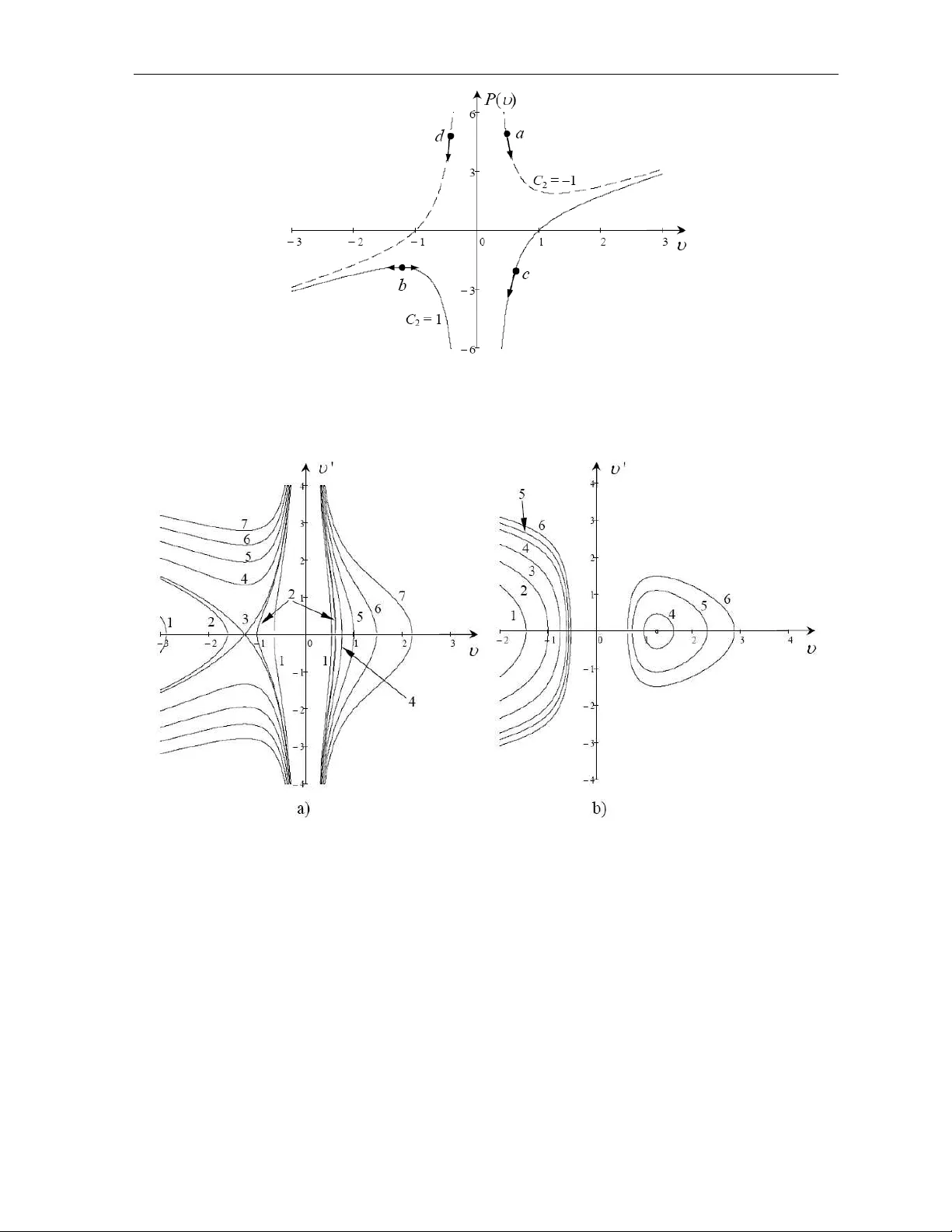
Symmetry , Integrabilit y and Geometry: Metho ds and Applications SIGMA 4 (2008), 073, 19 pages Solutions Classif ication to the Extended Reduced Ostro vsky Equation Y ury A. STEP ANY ANTS A ustr alian Nucle ar Scienc e and T e chnolo gy, Or ganisation PMB 1, Menai (Sydney), NSW, 2234, Austr alia E-mail: yuas50@gmail.c om Receiv ed July 14, 2008, in f inal form Octob er 13, 2008; Published online October 26, 2008 Original article is a v ailable at http://www.emis.de/journals/SIGMA/2008/073/ Abstract. An alternativ e to the P ark es’ approac h [ SIGMA 4 (2008), 053, 17 pages ] is suggested for the solutions categorization to the extended reduced Ostrovsky equation (the exR OE in Park es’ terminology). The approach is based on the application of the qualitative theory of dif ferential equations whic h includes a mechanical analogy with the p oin t particle motion in a p otential f ield, the phase plane metho d, analysis of homo clinic tra jectories and the lik e. Suc h an approac h is seemed more vivid and free of some restrictions con tained in [ SIGMA 4 (2008), 053, 17 pages ]. Key wor ds: reduced Ostro vsky equation; mec hanical analogy; phase plane; p erio dic wa v es; solitary wa v es, compactons 2000 Mathematics Subje ct Classific ation: 35Q58; 35Q53; 35C05 1 In tro duction In pap er [ 1 ] E.J. Park es presented a categorization of solutions of the equation dubb ed the extended reduced Ostrovsky equation (exR OE). The equation s tudied has the form ∂ ∂ x  D 2 u + 1 2 pu 2 + β u  + q D u = 0 , where D = ∂ ∂ t + u ∂ ∂ x (1) with p , q , and β b eing constan t co ef f icien ts. This equation w as deriv ed from the Hirota– Satsuma-t yp e shallow w ater w a v e equation considered in [ 2 ] (for details see [ 1 ]). F or stationary solutions, i.e. solutions in the form of trav elling w a v es depending only on one v ariable χ = x − V t − x 0 , this equation reduces to the simple third-order ODE: d dχ  w d dχ  w dw dχ  + 1 2 pw 2 + ( pV + β ) w  + q w dw dχ = 0 , (2) where V stands for the w a v e sp eed and w = u − V . (Note, that in many contemporary pap ers including [ 1 ] authors call suc h solutions simply “trav elling-wa v e solutions”. Suc h terminology seems not go o d as nonstationary propagating wa v es also are trav elling wa v es. The term “sta- tionary wa v es” widely used earlier seems more adequate for the wa v es considered here.) In pap er [ 1 ], equation ( 2 ) was reduced b y means of a series of transformations of dep endent and indep enden t v ariables to an auxiliary equation whose solutions w ere actually categorized sub ject to some restrictions on the equation co ef f icients, viz.: p + q 6 = 0 , q V − β 6 = 0 (one more restriction on the constant of integration for that auxiliary equation, B = 0, w as used in [ 1 ]). Under these restrictions, solutions to equation ( 2 ) w ere found in analytical form 2 Y.A. Stepany an ts and corresp onding w av e prof iles were illustrated graphically . Among solutions obtained there are b oth perio dic and solitary t yp e solutions including m ultiv alued loop perio dic wa v es and lo op-solitons. Similar lo op solutions to exR OE and some other equations w ere earlier obtained by Ji-Bin Li [ 3 ] who came to the conclusion that loop solutions actually are compound solutions whic h consist of three dif feren t indep endent branc hes. These branches ma y b e used in v arious combi- nations represen ting sev eral t yp es of stationary propagating singular w a v es (w a ves with inf inite gradien ts). This conclusion completely coincides with the conclusion of pap er [ 4 ] where a com- plete classif ication of stationary solutions of R OE w as presen ted. ROE derived b y L.A. Ostro v- sky [ 5 ] in 1978 as a mo del for the description of long wa ves in a rotating o cean (see [ 4 ] and references therein) can be treated as a particular case of exROE with p = q and β = 0 (see [ 1 ]). Belo w an analysis of stationary solutions to equation ( 2 ) is presented by the direct metho d a voiding any redundant transformations of v ariables. The metho d used is based on the phase plane concept and analogy of the equation studied with the Newtonian equation for the p oin t particle in a p otential f ield. Suc h approach seems more vivid and free of aforemen tioned re- strictions. This w ork can b e considered also as complementary to pap er [ 1 ] as the analysis presen ted ma y be helpful in the understanding of basic prop erties of stationary solutions of equation ( 2 ). 2 Mec hanical analogy , p oten tial function and phase-plane metho d Equation ( 2 ) can b e integrated once resulting in w d dχ  w dw dχ  + 1 2 ( p + q ) w 2 + ( pV + β ) w = C 1 , (3) where C 1 is a constant of integration. By multiplying this equation by dw /dχ and integrating once again, the equation can b e reduced to the form of energy conserv ation for a p oint particle of unit mass mo ving in the p otential f ield P ( w ): 1 2  dw dχ  2 + P ( w ) = E , (4) where the ef fectiv e “p otential energy” as a function of “displacemen t” w is P ( w ) = p + q 6 w − C 1 w − C 2 w 2 , (5) and C 2 is another constan t of in tegration. The constant E = − ( pV + β ) / 2 pla ys a role of the total energy of the particle, i.e. the sum of the “kinetic energy”, K = (1 / 2)( dw /dχ ) 2 , and the “p oten tial energy”, P ( w ). As follo ws from equation ( 4 ), real solutions can exist only for E ≥ P ( w ). V arious cases of the p otential function ( 5 ) are considered b elo w and corresp onding b ounded solutions are constructed. Un b ounded solutions are not considered in this pap er as they are less in teresting from the ph ysical p oint of view; nevertheless, their qualitativ e b ehavior b ecomes clear from the general view of corresp onding phase p ortraits. 3 P articular case: p + q = 0 Consider f irst a particular case when the co ef f icien ts in equation ( 1 ) are such that p + q = 0. Note, this is one of the cases which were omitted from the consideration in pap er [ 1 ]. The Solutions Classif ication to the Extended Reduced Ostrovsky Equation 3 Figure 1. a) Poten tial function for the case p + q = 0, C 2 = 0 and tw o v alues of C 1 : C 1 = 1 (solid lines), and C 1 = − 1 (dashed lines). Two dots illustrate p ossible motions of p oint particles in the p otential f ield. b) Phase plane corresp onding to the p otential function with C 1 = 1 and dif ferent v alues of E . Line 1: E = − 1; line 2: E = − 0 . 5; lines 3: E = 0 . 5; lines 4: E = 1. p oten tial function ( 5 ) simplif ies in this case. Ho wev er, a v ariet y of sub cases can b e distinguished nev ertheless ev en in this case dep ending on the co ef f icients C 1 and C 2 . All these sub cases are studied in detail b elo w. 3a. If C 2 = 0, the p otential function represen ts a set of an tisymmetric hyperb olas located either in the f irst and third quadran ts or in the second and fourth quadran ts as sho wn in Fig. 1 a. The corresp onding phase plane ( w , w 0 ), where w 0 = dw /dχ , is shown in Fig. 1 b for C 1 = 1 (for C 1 = − 1 the phase plane is mirror symmetrical with resp ect to the v ertical axis). F or other v alues of C 1 phase p ortraits are qualitativ ely similar to that sho wn in Fig. 1 for C 1 = 1. Analysis of the phase p ortrait shows that there are no bounded solutions for an y p ositiv e E ; corresp onding tra jectories b oth in the left half and right half of the phase plane go to inf inity on w (see, e.g., lines 3 and 4 in Fig. 1 b). Mean while, solutions bounded on w do exist for negativ e v alues of E (i.e. for V > − β /p ), but they p ossess inf inite deriv atives when w = 0. Consider, for instance, motion of an af f ix along the line 2 in Fig. 1 b ( C 1 = 1) from w 0 = ∞ to wards the axis w where w 0 = 0. The qualitative character of the motion b ecomes clear if we interpret it in terms of “particle co ordinate” w and “particle velocity” w 0 treating ξ as the time. The motion originates at some “time” ξ 0 with inf inite deriv ative and zero “particle coordinate” w = 0. Then, the “particle co ordinate” w increases to some maximum v alue w max = − C 1 /E ( E < 0) as the “particle v elo cit y” is positive. Even tually it comes to the rest ha ving zero deriv ative w 0 = 0 and w = w max . Another indep endent branch of solution for the same v alue of E corresp onds to the af f ix motion along the line 1 from the previously describ ed rest p oint at axis w to wards w 0 = −∞ and w = 0. All b ounded analytical solutions for this case can b e presented in the universal implicit form: ξ ( y ) − ξ 0 = ±  arctan  r y 1 − y  − p y (1 − y )  , (6) where y = − E w /C 1 , ξ = − √ 2( − E ) 3 / 2 χ/C 1 and ξ 0 is an arbitrary constan t of in tegration. This solution consists of tw o indep enden t branches whic h corresp ond to signs plus or minus in fron t of the square brack ets in equation ( 6 ). Eac h branc h is def ined only on a compact support of axis ξ : either on − π / 2 ≤ ξ − ξ 0 ≤ 0 or on 0 ≤ ξ − ξ 0 ≤ π / 2 (see lines 1 and 1 0 in Fig. 2 ). With the appropriate choice of constan ts ξ 0 one can create a v ariety of dif ferent solutions, e.g., the V -shap e wa ve (see lines 2 and 2 0 ), or a smo oth-crest compacton, i.e. a comp ound solitary w av e def ined only for | ξ − ξ 0 | ≤ π / 2 (see lines 3 and 3 0 ). Using a translational in v ariance of 4 Y.A. Stepany an ts Figure 2. V arious particular solutions described b y equation ( 6 ). Figure 3. Maxim um of the compacton solution ( 6 ) against sp eed in the original v ariables, equation ( 7 ). Dashed v ertical line corresp onds to the limiting v alue of V = − β /p . The plot is generated for C 1 = p = β = 1. solutions and their independency of eac h other, one can create perio dic or even c haotic sequences of compactons randomly lo cated on axis ξ . The maximum of the function y ( ξ ), y max = 1, corresp onds in terms of w to w max = − C 1 /E . Using the relationship betw een w and the original v ariable u (see ab o ve), as well as the def inition of the constant E , one can deduce the relationship b etw een the w av e extreme v alue (wa ve maxim um) and its sp eed: u max = V − C 1 E = V + 2 C 1 pV + β . (7) T aking into accoun t that w e consider the case of C 1 = 1, and negativ e v alues of E are p ossible only when V > − β /p , the plot of u max ( V ) is such as presen ted in Fig. 3 . As follows from equation ( 7 ), a wa ve is en tirely negativ e ( u max < 0), when V < 1 2 p  p β 2 − 8 pC 1 − β  , pro vided that p < β 2 / (8 C 1 ). At greater v alues of V , the wa ve prof ile con tains both positive and negativ e pieces, and for certain v alue of V the total w av e “mass” I = R u ( χ ) dχ v anishes (the in tegral here is taken o ver the en tire domain where function u ( χ ) is def ined). Solutions Classif ication to the Extended Reduced Ostrovsky Equation 5 Figure 4. a) Poten tial function for the case p + q = 0, C 1 = 0 and tw o v alues of C 2 : C 2 = 1 (solid lines), and C 2 = − 1 (dashed lines). Two dots illustrate p ossible motions of p oint particles in the p otential f ield. b) Phase plane corresp onding to the p otential function with C 2 = 1 and dif ferent v alues of E . Line 1: E = − 1; line 2: E = − 0 . 5; lines 3: E = 0 . 5; lines 4: E = 1. All lines are symmetrical with resp ect to axis w 0 and are lab elled only in the left half of the phase plane. 3b. A similar analysis can b e carried out for the case when C 1 = 0, C 2 6 = 0. The p otential function in this case represen ts a set of symmetric quadratic hyperb olas located either in the f irst and second quadran ts or in the third and fourth quadran ts as sho wn in Fig. 4 a for C 2 = ± 1. The corresp onding phase plane is sho wn in Fig. 4 b for C 2 = 1 only (there are no b ounded solutions for C 2 = − 1, therefore this case is not considered here). F or other p ositive v alues of C 2 phase p ortraits are qualitatively similar to that sho wn in Fig. 4 b. Analysis of the phase p ortrait sho ws that there are no b ounded solutions for C 2 = − 1, as w ell as for C 2 = 1 and any p ositiv e E (see, e.g., lines 3 and 4 in Fig. 4 b); they exist how ever for C 2 = 1 and negative v alues of E , but p ossess inf inite deriv atives at some v alues of χ . In nor- malized v ariables y = ( − E /C 2 ) 1 / 2 w , ξ = − E (2 /C 2 ) 1 / 2 χ all p ossible solutions can b e presented in terms of indep endently chosen function branches describing a unit circle in one of the four quadran ts, i.e. ( ξ − ξ 0 ) 2 + y 2 = 1 , (8) where ξ 0 is an arbitrary constan t of integration. Pla ying with the constant ξ 0 one can create again a v ariety of compacton-type solutions including multi-v alued solutions. Some examples of solitary compacton solutions are shown in Fig. 5 a; they include N -shaped w av es, m ulti-v alued circle-shaped w av es and semicircle positive- p olarit y pulses (due to symmetry , the p olarit y of the f irst and last wa ves can b e in verted). In addition to those, v arious p erio dic and even c haotic comp ound wa ves can be easily constructed; one of the p ossible examples of a p erio dic solution is shown in Fig. 5 b. Each positive or negativ e half-p erio d of any w a ve consists of tw o indep endent branches originating at y = 0 and ending at y = ± 1. The same is true for the pulse-type solutions shown in Fig. 5 a; they consist of indep enden t symmetrical branc hes as shown, for example, for the semicircle pulse in Fig. 5 a where they are lab elled by sym b ols 1 and 2. The maximum of the function y ( ξ ), y max = 1, corresp onds in terms of w to the wa ve maxi- m um, w max = ( − C 2 /E ) 1 / 2 . Using a relationship b et ween w and the original v ariable u (see ab o v e), as well as def inition of the constan t E , one can deduce the relationship b et ween the 6 Y.A. Stepany an ts Figure 5. a) Some examples of pulse-type wa ves describ ed by equation ( 8 ): N -shap ed wa ve; circle w av e and semicircle compacton. b) One of the examples of a p erio dic w av e with inf inite deriv atives at y = 0, ξ = 2 n + 1, w here n is an en tire num b er. w av e maximum and its sp eed: u max = V + r − C 2 E = V + s 2 C 2 pV + β . (9) The plot of u max ( V ) is presented in Fig. 6 for V > − β /p in accordance with the c hosen constant C 2 = 1 and E < 0. As follows from equation ( 9 ), wa v e maximum (minim um) cannot b e less than the certain v alue, U max ( − U min ), which occurs at some sp eed V 1 , where U max = 1 p "  C 2 p 2 2  1 / 3 − β # + 2  C 2 2 p  1 / 3 , V 1 = 1 p "  C 2 p 2 2  1 / 3 − β # . F or all p ossible v alues of wa ve maximum u max > U max , tw o v alues of wa ve sp eed are pos- sible, i.e. t wo w av es of the very same “amplitude” can propagate with dif feren t sp eeds. This is illustrated b y horizon tal dashed line in Fig. 6 dra wn for u max = 2 . 5. The same is true for w a ves of negative polarity . 3c. Consider no w the case when b oth C 1 and C 2 are nonzero but p + q is still zero. There are in general four p ossible combinations of signs of the parameters C 1 and C 2 : i) C 1 > 0 , C 2 > 0; ii) C 1 < 0 , C 2 > 0; iii) C 1 > 0 , C 2 < 0; iv) C 1 < 0 , C 2 < 0 . The shape of the p oten tial function P ( w ) and corresp onding solutions are dif feren t for all these cases. Ho w ever, among them there are only tw o qualitatively dif feren t and indep endent cases, whereas the t wo others can b e obtained from those tw o cases using simple symmetry reasons. This statemen t is illustrated by Fig. 7 , where the p otential relief is shown for all four aforemen tioned cases i)–iv). As one can see from Fig. 7 , cases i) and ii), as w ell as iii) and iv), are mirror symmetrical coun terparts of each other with resp ect to the vertical axis. This implies that solutions for the cases i) and ii), and corresp ondingly , iii) and iv), are related by the simple sign in terchange Solutions Classif ication to the Extended Reduced Ostrovsky Equation 7 Figure 6. Dep endence of the w av e maxim um on sp eed in original v ariables, equation ( 9 ), as follo ws from solution ( 8 ). Dashed v ertical line corresp onds to V = − β /p . The plot is generated for C 2 = p = β = 1. Figure 7. Poten tial relief for the four dif ferent cases, i)–iv), of v arious signs of constants C 1 and C 2 . The plot w as generated for C 1 = ± 1, C 2 = ± 0 . 1. op eration, i.e. w i) = − w ii) , w iii) = − w iv) . Therefore, b elow only t wo qualitativ ely dif ferent cases are considered in detail, namely the cases i) and iii). Case i) is c haracterized by an inf inite p otential well at the origin, w = 0. This singularit y in the p otential function corresp onds to the existence of a singular straight line w = 0 on the phase plane (see Fig. 8 ). On b oth sides from this singular line there are qualitativ ely similar tra jectories whic h corresp ond to b ounded solutions having inf inite deriv atives at the edges. Quan titative dif ference b et ween the “left-hand side solutions” and “right-hand side solutions”, apart of their dif feren t p olarit y , is the former solutions (of negative p olarity , w ≤ 0) exist for E ≤ P max , whereas the latter ones (of p ositive p olarity , w ≥ 0) exist for E ≤ 0. The p otential function has a maximum P max = C 2 1 / (4 C 2 ) at w = − 2 C 2 /C 1 . There are no b ounded solutions for E > P max . Consider f irst bounded solutions whic h corresp ond to tra jectories sho wn in the left half- plane, w ≤ 0, in Fig. 8 . F or a positive v alue of the parameter E in the range 0 ≤ E ≤ P max , the analytical solution can b e presented in the form ξ ( y ) = ± 2 p Q " p ( y + 2 Q ) 2 − 4 Q ( Q − 1) − 2 Q ln y + 2 Q + p ( y + 2 Q ) 2 − 4 Q ( Q − 1) 2 p Q ( Q − 1) # , (10) where ξ = χ √ 2 C 2 ( C 1 /C 2 ) 2 , y = w ( C 1 /C 2 ), Q = C 2 1 / (4 C 2 E ). 8 Y.A. Stepany an ts Figure 8. Phase portrait of equations ( 3 ), ( 4 ) for the case i) (only those tra jectories are sho wn whic h corresp ond to particle motion within the potential well in Fig. 7 a). Line 1: E = 2 . 5; line 2: E = 1; lines 3: E = − 1; line 4: E = − 2; line 4: E = − 5. The range of v ariability on ξ is: | ξ | ≤ 4 Q n 1 − p Q ln h  p Q + 1  / p Q − 1 io , whereas y v aries in the range − 2 h Q − p Q ( Q − 1) i ≤ y ≤ 0 . The relationship b etw een the w av e minimum and its sp eed is: u min = V + C 1 pV + β + s 2 C 2 pV + β  C 2 1 2 C 2 ( pV + β ) + 1  , (11) where pV + β < 0 as E > 0. If E < 0, then the solution is ξ ( y ) = ± 2 p − Q " p 4 Q ( Q − 1) − ( y + 2 Q ) 2 + 2 Q arctan y + 2 Q p 4 Q ( Q − 1) − ( y + 2 Q ) 2 ! + π Q # . (12) The range of v ariabilit y on ξ is: | ξ | ≤ − 4 Q  1 + √ − Q  arctan √ − Q − π / 2  , whereas y v aries in the range − 2 h Q + p Q ( Q − 1) i ≤ y ≤ 0. The relationship b etw een the wa ve minimum and its sp eed is also given b y equation ( 11 ), but with pV + β > 0. Tw o sp ecial cases of solution ( 10 ) can b e men tioned. When Q = 1 ( E = P max ), solution ( 10 ) with the appropriate c hoice of the integration constan t reduces to ξ ( y ) = ± 4 h y 2 − ln  1 + y 2 i . (13) Solutions Classif ication to the Extended Reduced Ostrovsky Equation 9 This solution is unbounded on ξ , i.e. it is def ined in the range: | ξ | ≤ ∞ . How ever, the solution is b ounded on y : − 2 ≤ y ≤ 0. The relationship b etw een the wa ve minim um and its sp eed is simple as b oth of them are constant v alues in this sp ecial case: V = − 1 p  β + C 2 1 2 C 2  , u min = V − 2 C 2 C 1 = − 1 p  β + C 2 1 2 C 2 + 2 p C 2 C 1  . (14) Another sp ecial case corresp onds to Q = ∞ ( E = 0); in this case equation ( 10 ) after appro- priate choice of in tegration constan t reduces to: ξ ( y ) = ± 2 3 p y + 1( y − 2) . (15) The range of v ariabilit y on ξ is: | ξ | ≤ 4 / 3, whereas y v aries in the range: − 1 ≤ y ≤ 0. The relationship b etw een the w a ve minimum and its sp eed is also v ery simple as b oth of them are again constants but dif ferent from those given b y equation ( 14 ); in this case they are: V = − β p , u min = V − C 2 C 1 = −  β p + C 2 C 1  . Bounded solutions corresp onding to the tra jectories shown in the right half-plane in Fig. 8 with w ≥ 0, exist only for negativ e E ; they are giv en by equation ( 12 ), but with the dif feren t range of v ariabilit y of y : 0 ≤ y ≤ 2 h − Q + p Q ( Q − 1) i . The relationship b etw een the w av e maxim um and its speed is giv en again by equation ( 11 ) where u max should b e substituted instead of u min and pV + β > 0 as E < 0 for these solutions. Solutions ( 10 ), ( 12 ), ( 13 ) and ( 15 ) are shown in Fig. 9 . All these s olutions are of the com- pacton t yp e; they consist of tw o indep endent branches whic h can be matched dif ferently or unmatc hed at all. Lines 2 and 2 0 represen t an example when t wo branc hes are matched so that they form a semi-ov al; lines 3 and 3 0 represen t another example when t wo branc hes are matched so that they form an inv erted “seagull”. On the basis of these “elementary” solutions, v arious complex comp ound solutions can b e constructed including p erio dic or chaotic stationary w a ves. The dashed line 1 in the f igure corresp onds to E = 0 ( Q = 8). Another branch of the solution with the same v alue of E = 0 represents a solution of p ositive p olarit y whic h is un b ounded b oth on ξ and y . F or positive v alues of E , solutions of negative p olarity b ecome wider and of greater “amplitude” (see line 2). When E further increases and approaches P max , the solution b ecomes inf initely wide, but its minim um go es to − 2. In the limiting case E = P max ( Q = 1) t wo indep enden t branches of the solution can b e matched dif feren tly as sho wn by dashed-dotted lines 3 and 3 0 in Fig. 9 . The solution v anishes in this case when ξ = 0 and go es to − 2 when ξ → ±∞ ; this situation is describ ed by equation ( 13 ). F or the negativ e E there are t w o families of solutions: negativ e one, corresp onding to the left-hand side tra jectories in Fig. 8 , and p ositiv e one, corresp onding to the righ t-hand side tra jectories. When E , b eing negativ e, increases in absolute v alue ( Q v aries from −∞ to 0 − ), solutions depart from the line 1 in Fig. 9 and gradually squeeze to the origin (see line 4 for instance). F or the same v alues of negativ e E , positive solutions originated at inf inity also gradually shrink and collapse in the origin (lines 6 and 5 demonstrate this tendency). Consider no w the case iii) shown in Fig. 7 b. The p otential function in this case has only one w ell of a f inite depth so that P min = C 2 1 / (4 C 2 ) at w = − 2 C 2 /C 1 , where C 2 is negative now. There are no b ounded solutions for negativ e w; they exist how ever for positive w and E v arying in the range P min ≤ E < 0. The f inite v alue of the p otential minim um corresp onds to the equilibrium p oin t of the centre t yp e in the phase plane. There is also a family of closed tra jectories for the abov e indicated range of E v ariation (see Fig. 10 ); these tra jectories correspond to p erio dic solutions. 10 Y.A. Stepany an ts Figure 9. V arious solutions described by equations ( 10 ), ( 12 ), ( 13 ) and ( 15 ). Compactons of negative p olarit y: line 1: Q = ∞ ; lines 2 and 2 0 : Q = 2; lines 3 and 3 0 : Q = 1: line 4: Q = − 0 . 1. Compactons of p ositiv e p olarit y: line 5: Q = − 0 . 1; line 6: Q = − 0 . 25. Figure 10. Phase p ortrait of equations ( 3 ), ( 4 ) for the case 3c iii) (only those tra jectories are shown whic h corresp ond to particle motion within the p otential w ell in Fig. 7 b). The dot at the center of closed lines indicates an equilibrium p oint corresp onding to the p otential minim um ( E = − 2 . 5 for the chosen set of parameters: C 1 = 1, C 2 = − 0 . 1); line 1: E = − 2; line 2: E = − 1 . 5; line 3: E = − 1; line 4: E = − 0 . 5. As usual, closed tra jectories around the center ( E ≥ P min ) corresp ond to quasi-sin usoidal solutions. Whereas other closed tra jectories ( E > P min ) corresp ond to non-sinusoidal p erio dic w av es with smo oth crests and sharp narrow troughs. The larger is the v alue of E , the longer is the w a ve p erio d. The p erio d tends to inf init y when E → 0 − . The analytical form of this family of solutions is describ ed by the follo wing equation: ξ ( y ) = ± 2 p Q " p 4 Q ( Q − 1) − ( y + 2 Q ) 2 Solutions Classif ication to the Extended Reduced Ostrovsky Equation 11 Figure 11. V arious solutions describ ed b y equation ( 16 ). Line 1 (quasi-sinusoidal wa ve): Q = 1 . 01; line 2: Q = 1 . 5; line 3: Q = 2; line 4: Q = 2 . 5. Dashed lines sho ws the equilibrium state y = − 2. + 2 Q arctan y + 2 Q p 4 Q ( Q − 1) − ( y + 2 Q ) 2 ! − π Q # , (16) where ξ = χ √ − 2 C 2 ( C 1 /C 2 ) 2 , y = w ( C 1 /C 2 ), Q = C 2 1 / (4 C 2 E ). Solution ( 16 ) is shown in Fig. 11 for dif feren t v alues of Q (note that the solution is negativ e in terms of y b ecause C 2 < 0). As follo ws from equation ( 16 ), y v aries in the range: − 2 h Q + p Q ( Q − 1) i ≤ y ≤ − 2 h Q − p Q ( Q − 1) i , whereas the dependence of wa ve p erio d Λ on Q is: Λ( Q ) = 8 π Q √ Q . The w av e p erio d v aries from 8 π to inf init y when Q increases from unit y to inf init y . F rom the extreme v alues of y (see ab o ve indicated range of its v ariability) one can deduce the dependences of w a ve maximum and minimu m on sp eed in the original v ariables. The corre- sp onding formulae are: u max , min ( V ) = V + C 1 pV + β ∓ 2 C 2 s 1 2 C 2 ( pV + β )  C 2 1 2 C 2 ( pV + β ) + 1  , (17) where the upp er sign in front of the ro ot corresp onds to the wa ve maximum and low er sign – to the wa v e minimum. These dep endences are plotted in Fig. 12 for V > − β /p in accordance with the c hosen v alues of constan ts C 1 = 1, C 2 = − 0 . 1 and E < 0. The asymptote V = − β /p is sho wn in the f igure by the vertical dashed line. As follows from equation ( 15 ), wa v e maximum cannot b e less than the certain v alue, U max , which occurs at some sp eed V 1 sho wn in Fig. 12 . F or all p ossible v alues of wa ve maximum u max > U max , tw o v alues of wa ve sp eed are pos- sible, i.e. t wo p erio dic w av es of the same maxim um (but not minimum!) can propagate with dif feren t sp eeds. This is illustrated by the horizon tal dashed line shown in Fig. 12 and drawn for u max = 2 . 5. In original v ariables quasi-sinusoidal w av es exist when the sp eed is close to its limiting v alue V max = − 1 p  C 2 1 2 C 2 + β  ; there are no w av es with greater sp eed. When V ≤ V max , the w av e minim um and maxim um are close to each other. Then, when the speed decreases, the gap b etw een w av e maximum and minim um gradually increases and go es to inf init y when the sp eed approaches its minim um v alue V min = − β /p . 12 Y.A. Stepany an ts Figure 12. Dep endences of w av e maxim um (solid line) and minimum (dashed-dotted line) on sp eed in the original v ariables, equation ( 17 ), as follo ws from the solution ( 16 ). Dashed vertical line corresp onds to V = − β /p . The plot is generated for C 1 = 1, C 2 = − 0 . 1 and p = β = 1. 4 General case: p + q 6 = 0 Consider no w a more general case when the coef f icien ts in equation ( 1 ) are such that p + q 6 = 0. The basic equation ( 4 ) can be presen ted in the new v ariables η = ( p + q ) χ/ 6 and v = ( p + q ) w / 6 with the same constan t of in tegration E = − ( pV + β ) / 2, but with new ef fective potential function P ( v ) = v − C 1 v − C 2 v 2 . (18) The p otential function is monotonic when C 1 = C 2 = 0, and there are no b ounded solutions in this case. Bounded solutions ma y exist if at least one of these constan ts is nonzero. Below w e presen t p ossible forms of the p oten tial function and corresp onding phase p ortraits of b ounded solutions for v arious relationships b etw een constan ts C 1 and C 2 . Qualitativ ely all these cases are similar to those whic h hav e b een describ ed already in the previous section, therefore we omit the detailed analysis and do not present analytical solutions as they can b e obtained straigh tforwardly and expressed in te rms of elliptic functions. 4a . If C 2 = 0, the p otential function represents a set of antisymmetric hyperb olas located either in the f irst and third quadrants when C 1 = − 1, or in the second and fourth quadran ts when C 1 = 1; this is sho wn in Fig. 13 . F or the case of C 1 = 1 only bounded solutions of a compacton t yp e are possible for p ositiv e v . Suc h solutions corresp ond to the motion of particle c sho wn in the f igure down to the p otential w ell. This family of pulse-type solutions exist b oth for negative and p ositiv e E ; all of them are b ounded from the top with the maxim um v alues dep ending on E , hav e zero minim um v alues and inf inite deriv atives when v = 0. Corresp onding phase plane is presen ted in Fig. 14 a. F or the case of C 1 = − 1 there are tw o p ossibilities: i) there is a family of compacton-type solutions with v ≤ 0; they corresp ond to the motion of the particle b down to the p otential well (particle motion to the left from the top of the “hill” corresponds to un b ounded solutions). P os- sible v alues of particle energy E v ary for such motions from minus inf inity to P max = − 2 √ − C 1 , where P max is the lo cal maximum of the low er branc h of the potential function (see Fig. 13 ). The phase p ortrait of such motions is sho wn in the left half of the phase plane in Fig. 14 b. ii) Another possibility app ears for the particle motion within the p otential well shown in the f irst quadrant of Fig. 13 (see the particle a ). Within this w ell all phase tra jectories are Solutions Classif ication to the Extended Reduced Ostrovsky Equation 13 Figure 13. Poten tial function for the case p + q 6 = 0, C 2 = 0 and tw o v alues of C 1 : C 1 = 1 (solid line), and C 1 = − 1 (dashed line). Dots a , b and c illustrate p ossible motion of a point particle in the potential f ield. Figure 14. a) Phase plane corresp onding to the p otential function with C 1 = 1 and v arious v alues of E . Line 1: E = − 2; lines 2: E = − 1; lines 3: E = 0; lines 4: E = 1; lines 5: E = 2. All tra jectories in the left half-plane corresp ond to unbounded solutions. b) Phase plane corresponding to the p otential function with C 1 = − 1 and v arious v alues of E . Line 1: E = − 4; lines 2: E = − 3; lines 3: E = − 2; lines 4: E = − 1; lines 5: E = 2 . 1; lines 6: E = 2 . 5; lines 7: E = 3. closed and corresp onding solutions are b ounded and p erio dical; they can b e expressed in terms of elliptic functions. The phase p ortrait of such motions is shown in the righ t half of the phase plane in Fig. 14 b. 4b . If C 1 = 0, but C 2 6 = 0, the p otential function also represents a set of antisymmetric h yp erb olas lo cated either in the third quadrant and right half-plane in Fig. 15 when C 2 = 1, or in the f irst quadrant and left half-plane of that f igure when C 2 = − 1. F or the case of C 2 = 1 there are tw o p ossibilities: i) there is a family of compacton-type solutions with v ≤ 0; they corresp ond to the motion of the particle b down to the p otential well 14 Y.A. Stepany an ts Figure 15. Poten tial function for the case p + q 6 = 0, C 1 = 0 and tw o v alues of C 2 : C 2 = 1 (solid lines), and C 2 = − 1 (dashed lines). Dots a , b , c and d illustrate p ossible motion of a p oint particle in the p oten tial f ield. Figure 16. Phase plane corresponding to the potential function ( 18 ) with C 1 = 0. a) C 2 = 1 and v arious v alues of E . Lines 1: E = − 3; lines 2: E = − 2; lines 3: E = − 1 . 89; lines 4: E = − 1; lines 5: E = 0; lines 6: E = 1; lines 7: E = 2. b) C 2 = − 1 and v arious v alues of E . Line 1: E = − 1; line 2: E = 0; line 3: E = 1; lines 4: E = 2; lines 5: E = 2 . 5; lines 6: E = 3. All tra jectories in the left half-plane corresp ond to unbounded solutions. (particle motion to the left from the top of the “hill” corresp onds to un b ounded solutions). Possi- ble v alues of particle energy E v ary for suc h motions from min us inf init y to P max = 3( − C 2 / 4) 1 / 3 , where P max is the lo cal maxim um of the left branc h of the p oten tial function (see Fig. 15 ). The phase p ortrait of suc h motions is shown in the left half-plane in Fig. 16 a. ii) Another family of compacton-type solutions exist with v ≥ 0; they correspond to the motion of the particle c do wn to the p otential w ell. Possible v alues of particle energy E for suc h motions v ary from min us to plus inf init y . Corresponding phase plane is presented in the right half-plane in Fig. 16 a. Solutions Classif ication to the Extended Reduced Ostrovsky Equation 15 Figure 17. P oten tial function for the case p + q 6 = 0. a) Sup ercritical case: C 1 = − 1 and tw o v alues of C 2 : C 2 = 1 (solid lines), and C 2 = − 1 (dashed lines); b) marginal case: C 1 = − 3 and the same tw o v alues of C 2 ; c) subcritical case: C 1 = − 5 and the same t wo v alues of C 2 (in the last case the horizontal and vertical scales are doubled). F or the case of C 2 = − 1 b ounded solutions are smo oth p erio dic wa ves whic h corresp ond to the particle oscillations in the p oten tial well shown in the f irst quadrant in Fig. 15 . Energy is p ositiv e for suc h motion and v aries from P min = 3( − C 2 / 4) 1 / 3 , where P min is the local minimum of the righ t branc h of the potential function (see Fig. 15 ) to inf inity . Analytical solution for suc h w av es can b e also expressed in terms of cum b ersome elliptic functions. Corresp onding phase plane is presented in Fig. 16 b. 4c . Consider now the case when both C 1 6 = 0 and C 2 6 = 0. The shap e of the p oten tial function is more complex in this case in general and dep ends on the relationship b etw een the constan ts C 1 and C 2 . The n umber and v alues of the p otential extrema are determined by the n umber of real ro ots of the equation P 0 ( v ) = 0, where prime denotes the deriv ative on v . This condition yields (see equation ( 18 )): v 3 + C 1 v + 2 C 2 = 0 . F or real constants C 1 and C 2 this equation alwa ys has at least one real ro ot. The real ro ot is single when C 1 ≥ C cr 1 ≡ − 3 C 2 / 3 2 ; its v alue is giv en b y the expression v =  q ( C 1 / 3) 3 + C 2 2 − C 2  1 / 3 − ( C 1 / 3)  q ( C 1 / 3) 3 + C 2 2 − C 2  − 1 / 3 . F or the case C 1 > C cr 1 , p ossible qualitative conf igurations of the p otential function are sho wn in Fig. 17 a for the particular choices of constan ts: C 1 = − 1 and C 2 = ± 1. There is only one 16 Y.A. Stepany an ts Figure 18. Phase plane corresp onding to the marginal case, C 1 = C cr 1 . a) C 1 = − 3, C 2 = − 1. Line 1: E = − 3 . 05; line 2: E = − 3; line 3: E = − 2 . 9; line 4: E = − 2; line 5: E = 3 . 8; line 6: E = 4; line 7: E = 4 . 5. All tra jectories in the left half-plane correspond to un b ounded solutions. b) C 1 = − 3, C 2 = 1. Line 1: E = − 5; lines 2: E = − 4; lines 3: E = − 3 . 75; lines 4: E = − 3 . 5; line 5: E = 2 . 75; line 6: E = 3; line 7: E = 3 . 25; line 8: E = 3 . 5. lo cal minimum at the righ t branc h of the p otential function for C 2 = − 1 and a lo cal maxim um at the left branch of the potential function for C 2 = 1. Almost the same conf iguration of the p oten tial function o ccurs for the marginal case C 1 = C cr 1 , as sho wn in Fig. 17 b, ho wev er one more lo cal extremum app ears – on the left branch when C 2 = − 1 and on the righ t branc h when C 2 = 1. In the case C 1 < C cr 1 the p otential function is shown in Fig. 17 c; there are three lo cal extrema of the p oten tial function for any v alue of C 2 = ± 1. The p otential conf iguration in the sup ercritical case C 1 > C cr 1 qualitativ ely is similar to the case sho wn in Fig. 15 , therefore the corresp onding phase portraits are similar to those sho wn in Fig. 16 . In the marginal case, C 1 = C cr 1 , the p otential conf iguration is also similar to those tw o cases mentioned ab ov e, how ever there are some p eculiarities in the phase planes ref lecting the app earance of embry os of new equilibrium p oints. Corresp onding phase p ortraits are shown in Fig. 18 . The embry os app ear in the vicinity of E = − 3 in Fig. 18 a and in the vicinity of E = 3 in Fig. 18 b. In the sub critical case C 1 < C cr 1 the situation is dif ferent from the previous ones and should b e considered separately . In the case of C 2 = − 1, there are tw o p otential wells, one of a f inite depth on the left branc h of function P ( v ) and another inf initely deep and wide w ell but b ounded from the b ottom on the right branc h of function P ( v ) (see Fig. 17 c). F or the f irst p otential well there is a family of closed tra jectories in the phase plane corre- sp onding to p erio dic solutions with the parameter E v arying b etw een the lo cal minimum and maxim um of the potential function; these solutions are describ ed b y elliptic functions. All closed tra jectories are bounded by the lo op of separatrix designated by symbol 3 in Fig. 19 a. T ra jecto- ries inside the separatrix loop next to center corresp ond to quasi-sinusoidal wa ves, and the loop of the separatrix corresp onds to the solitary wa v e (soliton) whic h can be treated as the limiting case of p erio dic w a ves. The soliton shap e is describ ed by the follo wing implicit formula: η = ± √ 2  v 1 2 √ v 2 − v 1 ln  √ v 2 − v 1 + √ v 2 − v √ v 2 − v 1 − √ v 2 − v  + √ v 2 − v  , v 1 ≤ v ≤ v 2 , (19) Solutions Classif ication to the Extended Reduced Ostrovsky Equation 17 Figure 19. Phase plane corresponding to the sub critical case C 1 < C cr 1 . a) C 1 = − 5, C 2 = − 1. Line 1: E = − 6; lines 2: E = − 5; line 3: E = − 4 . 25; lines 4: E = − 4; line 5: E = 4 . 7; line 6: E = 5; line 7: E = 6; line 8: E = 8. All tra jectories in the left half-plane outside of the closed lo op of separatrix corresp ond to unbounded solutions. b) C 1 = − 5, C 2 = 1. Line 1: E = − 7; line 2: E = − 5; lines 3: E = − 4 . 657; lines 4: E = − 4; lines 5: E = 4 . 3; line 6: E = 5; lines 7: E = 6 . 656; lines 8: E = 7. Figure 20. Soliton solutions on pedestals as desc rib ed b y equations ( 19 ). where v 1 , 2 = −  C 1 ∓ p C 2 1 − 3 E C 2  /E , ( v 1 < v 2 ) and E = P max ( C 1 , C 2 ), where P max ( C 1 , C 2 ) is the v alue of the potential local maxim um shown in the left half-plane of Fig. 17 c. Solution ( 19 ) is shown in Fig. 20 a. In original v ariables function u describing soliton v aries in the range V + 6 v 1 p + q ≤ u ≤ V + 6 v 2 p + q ; th us, the soliton amplitude amoun ts A = 6 v 2 − v 1 p + q = 12 p + q p C 2 1 − 3 C 2 P max ( C 1 , C 2 ) P max ( C 1 , C 2 ) ; (20) The soliton velocity is V = − 1 p [ β + 2 P max ( C 1 , C 2 )] . (21) 18 Y.A. Stepany an ts Equations ( 20 ) and ( 21 ) allo w one to obtain a direct relationship b et w een the soliton’s v elo city and amplitude: A = − 24 p + q q C 2 1 + 3 2 C 2 ( pV + β ) pV + β . F or the second p oten tial well lo cated in the righ t half-plane of Fig. 17 c, there is another family of closed tra jectories in the phase plane corresp onding to p erio dic solutions with the parameter E v arying betw een the local minim um of the p otential function and inf inity; these tra jectories are shown in the right half-plane of Fig. 19 a. In the case of C 2 = 1, there is a shallo w p oten tial w e ll on the righ t branc h of function P ( v ) and one inf initely deep well at the origin where the potential function is singular. F or the shallo w w ell there is a family of closed tra jectories in the phase plane corresp onding to p erio dic solutions with the parameter E v arying b etw een the lo cal minimum and maximum of the p otential function. All suc h tra jectories are also b ounded b y the lo op of separatrix designated by symbol 7 in Fig. 19 b. The lo op of separatrix corresp onds to the solitary w av e whose shap e is describ ed b y the same implicit form ula ( 19 ), but with dif feren t v alues of constants C 1 , C 2 , E and P max ( C 1 , C 2 ), where P max ( C 1 , C 2 ) is the v alue of the p oten tial local maxim um sho wn in the right half-plane of Fig. 17 c. This solution is sho wn in Fig. 20 b. All ab ov e relationships b et ween soliton amplitude and v elo city , as well as b etw een soliton amplitude or velocity and constants C 1 and C 2 remain the same as ab o ve. F or the inf initely deep w ell at the origin there are t wo families of compactons with nonp ositiv e and nonnegativ e v alues; the phase plane for them is similar to that sho wn in Fig. 8 and solutions are similar to those sho wn in Fig. 9 . The en tire phase p ortrait of the system in the case of C 2 = 1 is sho wn in Fig. 19 b. Phase tra jectories corresponding to p ositiv e compactons are not sho wn in detail in that f igure because they are too close to eac h other and are in the narrow gap betw een the axis v 0 and external tw o unclosed branc hes of the separatix 7 (only one such tra jectory , line 5, is sho wn in Fig. 19 b; all other tra jectories are similar). 5 Conclusion As was sho wn in the pap er, the extended reduced Ostrovsky equation ( 1 ) p ossesses p erio dic and solitary t yp e solutions in general. There is a v ariety of solitary-w av e solutions including compactons with inf inite deriv ativ es at the edges, smooth solitons, and p erio dic wa ves. All compactons, how ever, actually are of the comp ound-type solutions, i.e., they consist of t wo or more non-smo oth branches. Among p erio dic w a ves dep ending on the equation parameters, there are also b oth smo oth solutions and comp ound-type solutions whic h consist of p erio dic sequences of non-smo oth branc hes (see, e.g., Fig. 5 b). Moreov er, using compacton solutions as the elementary blo cks, one can construct very complex comp ound solutions including sto c hastic stationary wa v es. The approach used in this pap er and based on the qualitative theory of dynamical systems is free from the limitations of pap er [ 1 ] and allo ws us to present a complete classif ication of all p ossible solutions of stationary exROE. In particular, solutions were obtained and analyzed in details for the case p + q = 0 that was out of consideration in pap er [ 1 ]. Another “prohibi- ted” combination of parameters, q V − β 6 = 0, that w as also out of consideration in pap er [ 1 ], do es not even app ear in our study . The approach exploited in the present pap er is based on a vivid mechanical analogy b etw een a particle mo ving in a sp ecial p otential f ield and considered stationary exROE. This approach allows one to observ e qualitativ ely an entire family of all p ossible solutions ev en without construction of particular exact solution. A similar approac h has b een exploited recen tly in application to the reduced Ostrovsky equation [ 4 , 3 ] and exROE [ 3 ], although in the last case, the complete solution classif ication was not considered. Solutions Classif ication to the Extended Reduced Ostrovsky Equation 19 References [1] Park es E.J., Periodic and solitary trav elling-w a ve solutions of an extended reduced Ostro vsky equation, SIGMA 4 (2008), 053, 17 pages, . [2] Morrison A.J., Park es E.J., The N -soliton solution of the mo dif ied generalised V akhnenko equation (a new nonlinear ev olution equation), Chaos Solitons F r actals 16 (2003), 13–26. [3] Li J.-B., Dynamical understanding of lo op soliton solution for several nonlinear wa ve equations, Sci. China Ser. A 50 (2007), 773–785. [4] Stepany ants Y.A., On stationary solutions of the reduced Ostrovsky equation: Periodic wa ves, compactons and comp ound solitons, Chaos Solitons F r actals 28 (2006), 193–204. [5] Ostrovsky L.A., Nonlinear internal wa ves in a rotating ocean, Oke anolo giya 18 (1978), 181–191 (Engl. transl: Oc e anolo gy 18 (1978), 119–125).