Evaluation and selection of models for out-of-sample prediction when the sample size is small relative to the complexity of the data-generating process

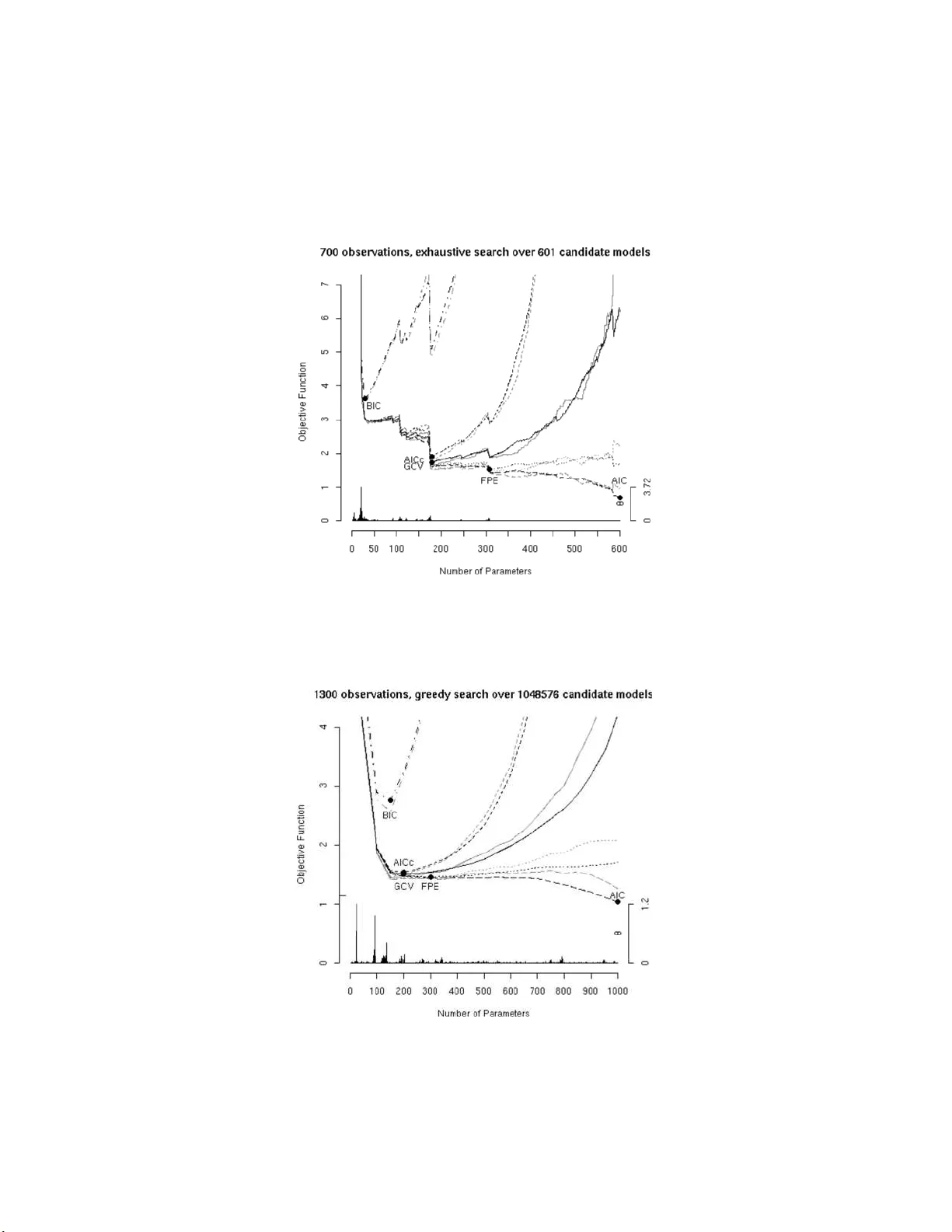
Bernoul li 14 (3), 2008, 661–690 DOI: 10.315 0/08-BEJ 127 Ev aluation and selection of mo dels for out-of-sample prediction when the sample size is small relativ e to the complexit y of the data-generating pro cess HANNES LEEB Dep artment of Statistics, Y ale University, 24 Hil l house A venue, New Haven, CT 06511, USA. E-mail: hannes.le eb@yale.e du In regressio n with random design, w e study the problem of selecting a mo del that p erforms w ell for out-of-sample prediction. W e do not assume that an y of the candidate mo dels under consideration are correct. Our analysis is based on explicit ﬁnite-sample results. Our main ﬁndings diﬀer from those of other analyses th at are based on traditional large-sample limit appro ximations b ecause we consider a situation where the sample size is small relative to the complexit y of t he data-generating pro cess, in th e sense that the num b er of parameters in a ‘goo d’ model is of the same order a s sample size . Also, w e allo w for the case where the num b er of candidate mo dels is (muc h) larger than sample size. Keywor ds: g eneralized cross val idation; large number of parameters and small sample size; model selection; nonparametric regression; out-of-sample prediction; S p criterion 1. In tro duction Some of to day’s mo st challenging statistical problems feature a large n um ber o f p oten- tially importa n t factors or v aria bles and a compara tiv ely small sample size. F or example, v an’t V eer et al. ( 2 002 ) successfully use gene expression proﬁling to pre dict recurr ence of breast cancer using a cla ssiﬁer compris e d o f 7 0 g e nes that are s elected fro m a total of ab out 2 5 000 based on a sample of size 78 ; see als o v an de Vijver et al. ( 2002 ). In such applications, the g oal of mo del selection is often not to ﬁnd ‘the corr ect model’, but rather a mo del that p erforms well for prediction. Mo reo ver, the num b er of explanatory v ariables (e.g., genes) in the selected mo del is often o f the sa me order as sample size and the num ber of candidate mo dels (e.g., subsets o f genes) is muc h la rger than sa mple size. W e consider one problem of that kind: regressio n with ra ndom design, where the true mo del is allow ed to b e inﬁnite-dimensional, and where the go a l is to ﬁnd a mo del with This is an electronic reprint of the original article published by the ISI/BS in Bernoul li , 2008, V ol. 14, No. 3, 661–690 . This reprint diﬀers from the original in p agi nation and typographic detail. 1350-7265 c  2008 ISI/BS 662 H. L e eb ‘go od’ out-of-sample predictive p erformance. 1 W e fo cus o n situations where the s ample size is relatively small, in the sense that the num b er of pa rameters in a ‘go o d’ mo del is of the sa me or der a s sample size. W e also allow for the ca s e where the n um b er o f candidate mo dels is (m uch) la rger than sample size. T o select a ‘go o d’ mo del, we esti- mate the p erformance o f candidate models and select the one with the b est estimated per formance. 1.1. Classical pro cedures Of course , mo del selection based o n es timated predictive p erformance has already b een extensively studied. Metho ds dev elo ped for that aim include the S p criterion (which can b e traced back to T ukey ( 1967 ); see also Ho c k ing ( 1976 ), Thompson ( 19 76a , 1976b )) ; the A k aike information criterion (AIC; Ak aike ( 1969 )); the ﬁnal prediction err or criterion (FPE; Ak aike ( 1970 )); the C p criterion of Mallows ( 1973 ); the generalized cross-v alidatio n criterion (GCV; Crav en a nd W ahba ( 19 78 )); or the sma ll-sample corr ected version of AIC (AICc; Hurvich and Tsai ( 1989 )). Minimizing these criteria ov er a class of ca ndidate mo dels leads to a mo del selection pro cedure that is conserv a tive (or ov er-c o nsisten t) in parametric s e ttings. 2 Alternatively , consistent mo del selection pr ocedures can be used, including the Bay esia n information criterion (BIC; Sch warz ( 197 8 )) or the minim um description length criterion (MDL; Rissanen ( 1978 )). F urther related metho ds include the prediction cr iterion (PC) of Amemiy a ( 1980 ) and the risk inﬂation criterion (RIC) of F oster and George ( 19 94 ). Existing perfor mance analyses of these mo del selectors do not give a clear picture as to what method is preferable. Consider a so-ca lled p ost-mo del-selection estimator, that is, a n estimator obtained by ﬁrs t se le c ting a model ba s ed on the training data and then ﬁtting the sele c ted mo del to the same training data by a metho d like least-squa res or maximum likelihoo d. In a parametric setting, Kempthorne ( 1984 ) s howed that a n y po st-model-sele c tio n estimato r is admissible within the class of a ll p ost-mo del- selection estimators (for squared er r or in-sample prediction loss). In large samples, it is w ell known that AIC and s imilar pro cedures are as ymptotically e ﬃcient (in a cer tain sense) if the true model is inﬁnite-dimensional, while BIC a nd rela ted metho ds are eﬃcient if the tr ue mo del is ﬁnite-dimensiona l (cf. Shao ( 199 7 ) and the references giv en therein). In ﬁnite samples, how ever, BIC can b e mor e eﬃcient than AIC (or vice versa), depending on sample size and on the unknown pa rameters, b oth in the parametric and the nonpar a- metric case s (cf. Kabaila ( 19 98 )). Y ang ( 2005 ) show ed that o ne cannot ﬁnd a pro cedure 1 Here, ‘out-of-sampl e prediction’ means prediction of new resp onses given hitherto unobserve d ex- planatory v ariables, whereas ‘in-sample prediction’ means prediction of new resp onses for the same explanatory v ariables as in the training data. 2 In a parametric setting, most mo del selectors can b e broadly classiﬁed as either consisten t or conserv ativ e: Consisten t mo del selectors ar e such that the probabilit y of selecting the most parsimonious correct mo del goes to 1 as sample size increases; conserv ative mo del selectors ar e not consistent, but suc h that the probabilit y of selecting an incorrect mo del goes to zero. Evaluation and sele ction of mo dels 663 that combines the strengths of AIC and BIC. In the case where the true mo del is ﬁnite- dimensional and as sample size gets large, consistent mo del selectors choose the smallest correct mo del with probability approa c hing 1, while conserv a tiv e ones do not; how ever, consistent mo del selec tors also lead to unbounded worst-case ris k , while the worst-case risk corres p onding to conser v ative pro cedures t ypically stays b ounded in large sa mples (cf. Leeb and P¨ otscher ( 2005 ) a s w ell as Leeb a nd P¨ otscher ( 2008 )). Hence, from the per - sp e c tive of existing per formance analyses, o ne cannot prefer one of these mo del selectors ov er the other in gener al b ecause the p erformance of a g iven mo del sele c to r dep e nds o n unknown par ameters a nd on sample size. 1.2. New approac hes In this paper , we ado pt a diﬀerent p erspec tive that provides new results and insig h ts. T o explain, we ﬁrst note that the a fo r emen tioned analyses that a re based on asymptotic considerations rely on lar g e-sample limit approximations that ‘kick in’ pr o vided that the sample siz e is ‘suﬃciently larg e’; the precise meaning o f ‘suﬃciently large’ typically depends on the underlying true data-genera ting pro cess and mor e complex pro cesses usually requir e larger samples. 3 In pra ctice, ho w ever, one often faces a v ery diﬀerent situation, namely one where the given sa mple siz e is relatively sma ll compar ed to the complexity o f the data-genera ting pro cess, for example, in the sense that the num b er of parameters in a ‘go od’ model is of the same order as sample size. In addition, the num ber of candidate models is often (muc h) lar ger than sample size. Here, w e adopt a framework that is sp eciﬁcally designed for s uc h scenar ios. W e ﬁnd that generalized cross-v alidation and T uk ey’s S p criterion p erform w ell in selecting a ‘go o d’ mo del, even if the c a ndidate mo dels are complex when compar ed to sample size and also if the n umber of candidate models is muc h la rger than sample size. More sp eciﬁcally , we show that the tr ue o ut-of-sample pre dictive p erformance o f a candidate mo del is well approximated b y generalize d cro ss-v alidation (or by the ob jec- tiv e function of the S p criterion) with high pro babilit y , uniformly ov er lar ge classes of candidate mo dels and uniformly ov e r h uge reg ions in pa rameter spa ce under very weak conditions; for details, see Theorem 3.4 and Corollary 3.5 . Moreov er , w e ﬁnd that several other mo del se lectors, including AIC and B IC, can be systematically defective when ev al- uating complex mo dels and that their p erformance can b e anyth ing fro m s a tisfactory or mildly sub optimal to co mpletely unreasonable, dep ending on unknown parameters. (This is in star k contrast to the well-known result that gener alized cross- v alidatio n and the S p criterion are a symptotically eq uiv alent to AIC – a res ult that holds asymptotically as the sample size gets lar g e r elativ e to the co mplexit y of the da ta -generating pro cess.) Our ﬁndings are ba sed o n explicit ﬁnite-sample results (cf. Theor em 3.2 and Corollar y 3 .3 ) and back ed up by simulation examples. 3 Here, the precise meaning of ‘complexit y’ depends on the details of the appro xim ation that is being considered. In many cases, ‘complexit y’ is r elated to the num b er of parameters or to smo othness conditions. 664 H. L e eb Conceptually , our approa ch is inspired b y Beran ( 1 9 96 ), Ber an and D ¨ um bgen ( 1998 ) and Bera n ( 20 00 ). The setting in these pap ers is similar to ours, in that the num b er o f explanatory v aria bles is of the same order a s sample size. Ho w ever, these pap ers con- sider regr ession with ﬁxed design a nd the fo cus is on estimating a diﬀerent p erformance measure, namely on the E uclidea n distance betw ee n the true lo cation parameter and the estimate. In that se tting, the p erformance of any estimator dep ends only o n the estima- tor itself and on the unknown true regr e ssion para meter. In contrast, we fo cus on the out-of-sample predictiv e p e rformance a nd w e consider ra ndom design. In our setting, the out-of-sample predictive p erformance of any estimator, in addition to dep ending on the estimator itself and the regr ession parameter, also dep ends on the design distribution, which is unknown. (If the num b er of des ign v a riables under consideration is suﬃcient ly small in r e la tion to sample size, the empirical distribution o f these design v a riables can be used as a proxy for the true design distribution. In the setting that we consider, how e v er, this do es not work b ecause the n um ber of desig n v ariables considered is no t necess arily small relative to sample size.) In the setting of Beran ( 19 9 6 ), a C p - o r AIC-like appro ac h to loss estimation is shown to work well. In our setting, we ﬁnd that C p and AIC do not work well and that a diﬀerent approach to per formance estimation is requir e d. A related dir ection of r e search was initiated by Barro n, Bir ge a nd Massar t ( 199 9 ) and further explored by Y a ng ( 19 99 ) and B a raud ( 20 02 ); see als o W egk amp ( 2003 ), as well as the references in these pap ers. Instead o f a ttemptin g to estimate the p erformance of ca ndidate models, these paper s provide ﬁnite-sa mple upper b ounds for the risk of po st-model-sele c tio n es timators that ar e based on minimizing an ob jectiv e function like pena lized maximum lik eliho o d o r p enalized least-squares, where the risk is deﬁned as the exp e cted Euclidean dista nce b et ween the true regression para meter and the es timato r, or some similar (known) distance measures, as in Baraud ( 20 02 ). Under s ome conditions and for C p - or AIC- like p enalty functions, these upp er b ounds give so-c alled ora cle in- equalities, stating that the true risk of the po st-model-sele c tio n estimator is within a constant multiple of the risk obtained by ﬁtting the minimal-risk mo del. (Note that the upper bound provided by such an oracle inequa lit y is not known in practice beca use it dep ends on the unknown regres s ion pa rameter.) Our results diﬀer from these in tw o impo r tan t aspects. First, we consider a diﬀerent ob jective, namely minimizing the o ut-of- sample prediction risk (where the p erformance o f an estimator , in addition to dep ending on the estimator and on the true regressio n parameter, also dep ends on the unknown distribution o f the design v ariables), a nd we fo cus on the case where the sample size is small relative to the complexity of the data-g enerating pro cess, a case where C p - or AIC- like ob jective functions do not p erform well. Second, instead of giving upp er bo unds, we show that the p erformance of the resulting po s t-model-selection estimator c a n actually be es timated in our setting. W e give ﬁnite-sample b ounds on the estimation erro r pro b- abilit y that dep end o nly on qua n tities that a re either known or that can b e estimated in a uniformly consistent fashion. T echnically , our pap er relies heavily on the results of Breiman a nd F r eedman ( 198 3 ), who giv e a lar ge-sample limit analysis of model selec tion by the S p criterion for the special case of nested c andidate mo dels. A precursor version of our pap er that was wr itten in 2005 was instead ba sed on the Ma r ˇ cenko–P astur la w (cf. Marˇ cenko and Pastur ( 19 67 )). Evaluation and sele ction of mo dels 665 1.3. Outline of this paper F or a sample of n observ atio ns fr o m some data-genera ting pro cess to b e sp eciﬁed later, we cons ider a co llection M n of candidate mo dels m ∈ M n with dimension | m | . (W e use the symbols m to deno te a candidate model and | m | to denote the n um ber of explanatory v ariables in the mo del m .) W e do not a ssume that the true r egression fun ction is co rrectly describ ed o r even w ell approximated by any of the candidate mo dels. Under mo del m , the resp onse is rela ted to a collection of | m | explanatory v ariables. The leading ca se of in terest is where the sample size is sma ll re la tiv e to the complexity o f the true data- generating pro cess, a case wher e ‘in teres ting’ models are such that | m | /n is lar ge, for example, | m | / n equals 0 . 1 , 0 . 5 or even 0 . 9 . W e fo cus on the case where the num b er of candidate mo dels, that is, # M n , is as larg e as, or muc h larger than, sample size. 4 Our ob jective is to select a mo del that perfor ms w e ll for out-of-sa mple prediction, that is, for predicting a new r e s ponse given hitherto unobserved explanatory v ariables . F o r a ﬁxed s e t of new explana tory v ariables, the mo del that p erforms b est for pr edicting the corresp onding resp onse can, and typically will, depend on the v a lues of these explanato ry v ariables (cf. Claes k ens a nd Hjor t ( 2003 )). T o iden tify a mo del that p erforms well in an ov era ll sense, we co nsider random desig n a nd we ev aluate a mo del’s p erformance by the conditional mean squared err or of the corresp onding predictor, wher e the co nditioning is on the tra ining sample. In other words, we sea rc h for a mo del that, when ﬁtted to the giv en training sa mple, p erforms well on a verage when repea tedly predicting new resp onses. (Of course, the case of rando m desig n also is a scenario of interest in its own right.) The conditional out-of-sample prediction error associa ted with mo del m is denoted b y ρ 2 ( m ) and w e consider the genera lized cross-v alidation criterion GCV ( m ) and T uk ey’s S p criterion S p ( m ), a s w ell as an auxilia ry criterion ˆ ρ 2 ( m ) (that will b e deﬁned later), a s estimators for ρ 2 ( m ); see Section 2 for the details. W e also consider other mo del selection criteria, namely the Ak aike information cr iterion AIC( m ), Hurvich and Tsai’s AICc( m ) and the ﬁnal prediction err or criterion FPE( m ), as well as the Bay es ian informa tio n criterion BIC( m ). A theoretica l analysis of the aforementioned criter ia is given in Section 3 , under the assumption that the data are sampled from a Gaussian distribution. W e ﬁrst give an explicit ﬁnite-sample analysis of the auxiliary criterion ˆ ρ 2 ( m ) in Section 3.1 . These results allow us to show that genera lized cross- v alidatio n and the S p criterion can be used to select a go od model with high pro ba bilit y , unifor mly ov er lar ge families of candidate mo dels and uniformly ov e r huge regions in parameter space under very w ea k conditions; see Section 3 .2 . Finally , the p erformance o f o ther mo del selectors is discussed in Section 3.3 . (On a technical level, the r esults in Section 3 rely hea vily on the assumption of Gaussianity , but we susp ect that s imilar ﬁndings migh t b e obtained in more general settings and our simul ation re s ults a ppear to supp ort this.) 4 Huber ( 1973 ) considers a related setting, where the dimension of the ov erall mo del, denoted b y k , is ﬁnite, but increases with n such that k /n → 0. He notes that settings where k /n and | m | /n are large “are unlike ly to yield a reasonably si m ple asymptotic theory” (cf . page 802 of that pap er). See also Portno y ( 1984 , 1985 ) and Mammen ( 1989 ). 666 H. L e eb The impact of our theoretica l results is demo nstrated in a simulation study in Section 4 , where we also consider no n-Gaussian samples. Our simulations include examples where a sample of size 1 300 is used to select a mo del from ov er a millio n ca ndidate mo dels. W e demonstrate that mo del selection by generalized cr oss-v alidation or the S p criterion per forms very well here and that the p erformance o f these mo del selector s is bas ica lly unaﬀected b y depar tures fro m normalit y . F or the o ther model selecto rs that w e consider, that is, for AIC( m ), AICc( m ), FPE( m ) and BIC( m ), we ﬁnd in the theoretical ana lysis and in the s im ulation examples that their perfor mance can be anything from sa tisfac to ry or mildly sub optimal to completely unreas o nable, dep ending on unknown parameters . The more technical parts o f the pr oofs are g iven in the Appendix. 2. Setting of the analysis Consider a resp onse y that is r e la ted to ex planatory v ariables x = ( x j ) ∞ j =1 b y y = ∞ X j =1 x j β j + u (1) for s ome β = ( β j ) ∞ j =1 . Throughout, we a ssume that the error u has mean zero and v ar iance σ 2 ≥ 0 , and that the (stochastic) s equence o f explana tory v aria bles x = ( x j ) ∞ j =1 has mean zero and v ariance/ co v ariance net Σ = [ E ( x i x j )] i,j ≥ 1 such that the series in ( 1 ) converges in squared mean. Moreover, we a lso assume that the explana tory v ariables x j , j ≥ 1, are each uncorr e la ted with the e rror u a nd that the x j ’s ar e no t p erfectly correla ted among themselves. 5 The unkno wn pa rameters here are the sequence of r e gression co eﬃcient s, the error v ariance and the v ar iance/cov aria nce net of the regres sors, that is, β , σ 2 and Σ. The (minimal) requirement, that the series in ( 1 ) conv er ges in squared mean, restricts β in a wa y that dep ends on Σ. F o r example, if Σ is such that the x j ’s hav e v aria nce 1 and are unco rrelated with each other, then it is required that β ∈ l 2 , that is, P j β 2 j < ∞ . (F or the case where the explanatory v aria bles ar e not cent ered, extensions of the results in this pap er a re g iven by Leeb ( 2007 ).) Consider a sample of size n from ( 1 ). The sample will b e denoted by ( Y , X ), where Y is the n -vector Y = ( y (1) , . . . , y ( n ) ) ′ , X is the n × ∞ net X = ( x (1) ′ , . . . , x ( n ) ′ ) ′ and ( y ( i ) , x ( i ) ) are indep e ndent and identically distr ibuted copies o f ( y , x ), as in ( 1 ). Let P n,β ,σ, Σ de- note the dis tr ibution of the sample ( Y , X ) and let E n,β ,σ, Σ denote the corresp onding exp e ctation op erator. Similarly , we wr ite V ar β ,σ, Σ [ y ] for the v ariance o f y in ( 1 ). 6 As estimators for β , we consider restricted least-squa res estimators cor respo nding to submo dels of the overall mo del ( 1 ), under which so me co e ﬃcients of β are re s tricted 5 In other words, w e require, f or each k ≥ 1 and integers j 1 < j 2 < · · · < j k , that ( x j 1 , . . . , x j k ) ′ is a random v ector with mean zero and positive deﬁnite v ariance/co v ariance matrix that is uncorrelated with u . 6 It should b e noted that P n,β ,σ, Σ , E n,β ,σ, Σ and V ar β ,σ, Σ [ y ], in addition to depending on the param- eters β , σ and Σ, also dep end on the actual distribution of ( y , x ) in ( 1 ); this dependence is not r eﬂected explicitly b y the notat ion. The distribution of ( y , x ) wi ll alw ays be clear from the con text. Evaluation and sele ction of mo dels 667 to zero. E ac h such submo del ca n b e identiﬁed by a 0-1 sequence m = ( m j ) ∞ j =1 , where m j = 0 if the j th co eﬃcient o f β is restricted to zero and m j = 1 otherwise; the n umber of unrestricted compo nen ts, that is, the num b er of 1’s in m , is denoted by | m | . Throug hout the pap er, we shall alwa ys a s sume that | m | < n − 1. 7 W e call | m | the order of the mo del m . The restricted lea st-squares estimator co rrespo nding to the mo del m is denoted by ˜ β ( m ) and is deﬁned as follo ws : ˜ β ( m ) is such that its j th component equals zero whenev er m j = 0 ; the | m | rema ining (unrestricted) compo nents of ˜ β ( m ) are obtained b y regre s sing Y on the corr esponding co lumns o f X . Based o n the sample ( Y , X ) , o ur ob jectiv e is to ﬁnd a ‘go o d’ mo del for out-of-sa mple prediction. T o this end, consider a new copy ( y ( f ) , x ( f ) ) of ( y , x ), as in ( 1 ), that is inde- pendent of ( Y , X ). Given a mo del m with | m | < n − 1 and the cor responding r estricted least-squar e s estimator ˜ β ( m ), we will use x ( f ) ′ ˜ β ( m ) a s a predictor for y ( f ) . T o ev a luate the per formance of this predictor, w e consider the conditional and unconditional mean squared prediction error s given by ρ 2 ( m ) = E n,β ,σ, Σ [( y ( f ) − x ( f ) ′ ˜ β ( m )) 2 k Y , X ] and R 2 ( m ) = E n,β ,σ, Σ [( y ( f ) − x ( f ) ′ ˜ β ( m )) 2 ] , resp ectiv ely . F or the conditional mea n squa red prediction error ρ 2 ( m ), note that the sample ( Y , X ) is k ept ﬁxed and the av erag e is taken only with resp ect to ( y ( f ) , x ( f ) ), so ρ 2 ( m ) is a function of ˜ β ( m ) − β . In particular, ρ 2 ( m ) can beco me large if either the mo del is to o co mplex (so that ˜ β ( m ) is not clo s e to β beca use of over-ﬁt), or if imp ortant explanatory v aria bles are no t included in the mo del (so that ˜ β ( m ) is not close to β because of under-ﬁt). Also, note that ρ 2 ( m ) = V a r n,θ ,σ, Σ [ y ( f ) − x ( f ) ′ ˜ β ( m ) k Y , X ] her e b ecause the mean of x ( f ) is zero. F or the case wher e the mea n of x ( f ) is not zero such that ρ 2 ( m ) = V ar n,θ ,σ, Σ [ y ( f ) − x ( f ) ′ ˜ β ( m ) k Y , X ] + ( E n,θ ,σ, Σ [ y ( f ) − x ( f ) ′ ˜ β ( m ) k Y , X ]) 2 , w e refer to Leeb ( 2007 ): ass uming that the sample is Gaussian a nd that the mo del includes an intercept, it is sho wn in that paper that the squared bias, that is, ( E n,θ ,σ, Σ [ y ( f ) − x ( f ) ′ ˜ β ( m ) | Y , X ]) 2 , is of smaller or der than the v a riance, that is, V ar n,θ ,σ, Σ [ y ( f ) − x ( f ) ′ ˜ β ( m ) k Y , X ]. Our main fo c us will b e on the conditional mea n squared prediction er ror, that is, ρ 2 ( m ), r ather than on the unconditiona l mean squa red prediction error , that is, R 2 ( m ), which is based on av era ging ov er hypothetical samples. Also, note tha t ρ 2 ( m ) dep ends o nly o n n , β , σ and Σ ; R 2 ( m ), o n the other ha nd, a lso depends on the actual distribution o f the random v ariables in ( 1 ). R emark 2.1. Instead o f R 2 ( m ) or ρ 2 ( m ), traditiona l la rge-sample limit analys es often consider error measures like the (unconditional) mean o f ( x ( f ) ′ β − x ( f ) ′ ˜ β ( m )) 2 , scaled by a parametric o r no npa rametric rate (dep ending on the setting). In a par ametric se tting, where the parameter β has o nly ﬁnitely many non-zer o comp onents, this is b ecause the 7 W e assume | m | < n − 1 f or the sak e of con ven ience; some of our results also hold fo r | m | < n , while others ev en hold for | m | ≤ n . 668 H. L e eb mean of ( x ( f ) ′ β − x ( f ) ′ ˜ β ( m )) 2 go es to zer o a t a r ate of 1 /n , provided that the model m is correct. Similar considerations apply in nonparametric settings under smo othness conditions, provided that the dimension of the mo del increase s a ppropriately with sample size. Considering the mean of ( x ( f ) ′ β − x ( f ) ′ ˜ β ( m )) 2 or of ( y ( f ) − x ( f ) ′ ˜ β ( m )) 2 is equiv alent, as far a s selecting a ‘go o d’ mo del is concerned, b ecause the tw o means diﬀer b y a ﬁxe d constant, namely the err o r v ariance σ 2 . The lack of sca ling by some rate in ρ 2 ( m ) and R 2 ( m ) is caused b y the fact that we do not a s sume a parametric mo del and we do not imp ose smo othness conditions in a no nparametric mo del b ecause such assumptions would mean that estimation erro r s go to ze ro as sample size increa ses. Instead, we use approximations that retain the ﬁnite-sample feature that estimation errors ar e p oten tially large b ecause the sample size is small relative to the complexity o f the data-genera ting pro cess. The conditional and unconditional mean squared prediction err ors depend on unkno wn parameters and thus m ust be estimated. F or a ca ndidate model m , we consider the generalized cross- v alidatio n criterion GCV ( m ), the S p criterion S p ( m ) and an auxiliary criterion ˆ ρ 2 ( m ), which are deﬁned as follows. Let GCV( m ) = (1 /n )RSS( m ) (1 − | m | /n ) 2 = RSS( m ) n − | m | n n − | m | . In the ab o v e displa y , RSS( m ) denotes the residual sum of squar e s obta ined by ﬁtting the mo del m , tha t is, RSS( m ) = P n i =1 ( y ( i ) − x ( i ) ′ ˜ β ( m )) 2 . The generalized cros s -v a lida tion criterion is closely related to the S p criterion, w hich is deﬁned by S p ( m ) = RSS( m ) n − | m | n − 1 n − 1 − | m | . F or technical reasons, we also consider a nother quantit y that is closely r elated to both GCV( m ) and S p ( m ), namely ˆ ρ 2 ( m ) = RSS( m ) n − | m | n + 1 n + 1 − | m | . F or most practica l purp oses, the diﬀerence b et ween GCV( m ) , S p ( m ) and ˆ ρ 2 ( m ) is neg- ligible. (Also, no te that GCV( m ), S p ( m ) and ˆ ρ 2 ( m ) are well deﬁned b ecause we always assume that | m | < n − 1 .) The o ther mo del selectors mentioned in the I ntro duction a re deﬁned in Section 3.3 . 3. Theoretical analysis In this section, we study the problem of estimating the conditional and unconditional mean squared prediction error in the case wher e the sample is drawn from a Gaussian distribution. W e hence a ssume throughout this section that the ra ndom v ariables in ( 1 ) Evaluation and sele ction of mo dels 669 are jointly normal. 8 Unless otherwise noted, we ﬁx para meters β , σ and Σ as in ( 1 ) a nd consider a ﬁxed sample size n and a ﬁxed mo del m with | m | < n − 1 . F or y a nd x a s in ( 1 ), set σ 2 ( m ) = V ar β ,σ, Σ [ y k x j : j ∈ N , m j = 1] . Note that σ 2 ( m ) is non-ra ndom b ecause the inv o lv ed random v a riables are jointly Gaus- sian, and that σ 2 ( m ) ≤ σ 2 (0) = V ar β ,σ, Σ [ y ]. 3.1. Finite-sam ple r esults The following result (whose ﬁrst statemen t is adapted fro m Breiman a nd F r eedman ( 1983 )) provides the ba sis for a ﬁnite-sample analys is. Prop osition 3.1. (i) The c onditional me an squar e d pr e diction err or ρ 2 ( m ) has the same distribution as 1 plus t he r atio of two indep endent chi-squar e d r andom variables with | m | and n − | m | + 1 de gr e es of fr e e dom, r esp e ctively, multiplie d by σ 2 ( m ) : ρ 2 ( m ) ∼ σ 2 ( m )  1 + χ 2 | m | χ 2 n −| m | +1  . (ii) The r esidual sum of squar es has t he same distribution as a chi-squar e d r andom variable with n − | m | de gr e es of fr e e dom, mult ip lie d by σ 2 ( m ) : RSS( m ) ∼ σ 2 ( m ) χ 2 n −| m | . Prop osition 3.1 immediately implies that the unconditional mean squa red prediction error R 2 ( m ) can b e computed ex plicitly as R 2 ( m ) = σ 2 ( m ) n − 1 n − 1 − | m | beca use w e alwa ys a s sume that | m | < n − 1 (recall the formu la for the mean of the F - distribution). This a lso g iv es the well-known result that S p ( m ) is an unbiased estimator for the unconditional mean squared prediction err or R 2 ( m ); the estimators GCV ( m ) and ˆ ρ 2 ( m ) for R 2 ( m ) ar e biased, but the bias is typically negligible. F or | m | < n − 3, we also get that the v ariance o f ρ 2 ( m ) is ﬁnite a nd g iv en by 2 σ 4 ( m ) | m | ( n − 1) ( n − | m | − 1) 2 ( n − | m | − 3) ≈ 2 n σ 4 ( m ) | m | /n (1 − | m | /n ) 3 . W e see that the conditional mean squared prediction er ror, that is, ρ 2 ( m ), is highly concentrated around its mean, that is, R 2 ( m ), provided only that n is larg e enough 8 Note that assuming the s ample to b e Gaussian entails that P n,β ,σ, Σ and E n,β ,σ, Σ , as well as V ar β ,σ, Σ [ y ], are uniquely determined b y the parameters in the subscript. 670 H. L e eb relative to σ 4 ( m ) / (1 − | m | /n ) 3 . This suggests that S p ( m ), GCV ( m ) a nd ˆ ρ 2 ( m ) ca n b e used to estimate not only R 2 ( m ), but als o the conditional mean s quared prediction error ρ 2 ( m ). In order to use these co nsiderations for model selection, w e need to establish that, say , ˆ ρ 2 ( m ) is close to ρ 2 ( m ) with high proba bilit y , not only for a ﬁxed mo del m , but for an ent ire collection of candidate mo dels. This is accomplished by the following theor em and the attending coro llary . Theorem 3.2. F or e ach ǫ > 0 , we have P n,β ,σ, Σ ( | ˆ ρ 2 ( m ) − ρ 2 ( m ) | > ǫ ) ≤ 4 exp  − n  1 − | m | n  Ψ  ǫ 2 σ 2 ( m )  1 − | m | n  , wher e Ψ( · ) is deﬁne d by Ψ( x ) = ( x/ ( x + 1)) 2 / 8 for x ≥ 0 . (In t he c ase σ 2 ( m ) = 0 , the upp er b ound is to b e interpr ete d as zer o.) F or ﬁxed ǫ > 0 , the upper b ound in Theorem 3.2 is of the fo r m 4 exp[ − nC ], where C is alwa ys po sitiv e. This upp er b ound is exp onen tially s mall in n , provided only tha t | m | /n is b ounded aw ay from 1 and σ 2 ( m ) is b ounded aw ay from inﬁnity . The upp er b ound depends o n the known quantities n , | m | /n and ǫ , a nd also on σ 2 ( m ), which is unknown. How ever, reca ll that σ 2 ( m ) is bo unded from above by σ 2 (0) = V ar β ,σ, Σ [ y ], that is , b y the v ariance of y in ( 1 ), whic h ca n b e r eadily estimated from the sample, for ex ample, by ( n − 1 ) − 1 P n i =1 ( y ( i ) − ¯ y ) 2 , where ¯ y denotes the mean of the r esponses y (1) , . . . , y ( n ) in the training sample. Thus, we see that the upp er b ound in Theorem 3.2 is exp onen tially small in n , provided only that bo th the complexity of the candidate mo del and the v ariance of the resp onse, that is, | m | and V a r β ,σ, Σ [ y ], ar e not to o larg e . These considerations, together with Bonfer r oni’s inequality , immediately lead to the following result. Corollary 3.3. Consider a (ﬁnite and non-empty) c ol le ction M n of c andidate mo dels and let r n = sup m ∈M n | m | /n . Then sup β ,σ, Σ as in ( 1 ) V ar β ,σ , Σ [ y ] ≤ c P n,β ,σ, Σ  sup m ∈M n | ˆ ρ 2 ( m ) − ρ 2 ( m ) | > ǫ  ≤ 4# M n exp[ − n (1 − r n )Ψ(( ǫ/ (2 c ))(1 − r n ))] for e ach ǫ > 0 and for e ach (ﬁ nite) c > 0 . (Her e, # M n denotes the n umb er of c andidate mo dels and Ψ( · ) is as in The or em 3.2 .) The upp er b ound given in Corolla ry 3.3 is o f the form 4 exp[ − nD + log # M n ], where the constant D > 0 depends on r n and c (for ﬁx e d ǫ > 0 ). In particular , the upper bo und is small provided only that the v ar iance of the resp onse, the complexity of the candidate mo dels and the n um ber of candidate mo dels are not to o larg e in relation to sample size. Evaluation and sele ction of mo dels 671 Clearly , results paralleling Theorem 3.2 and Corollar y 3 .3 ca n also b e derived when either gener alized cross- v alida tio n or the S p criterion, that is, GCV ( · ) or S p ( · ), are used instead of ˆ ρ 2 ( · ). The rea son for consider ing ˆ ρ 2 ( · ) here is that this estimator lea ds to the most simple and mos t revealing upp er bound. (In mo st practical cas e s , the distinction betw een ˆ ρ 2 ( m ), GCV( m ) and S p ( m ) is negligible an y w ay . In the App endix, we also give a v ariant of Theorem 3.2 with S p ( m ) a nd R 2 ( m ) r eplacing ˆ ρ 2 ( m ) and ρ 2 ( m ), resp ectiv ely; see Pr opositio n A.5 .) It s hould be noted that the uppe r b ound in T heo rem 3.2 do es not go to zero as ǫ g oes to inﬁnit y . (The same also applies to the upp er b ound in Cor ollary 3.3 , which is derived from that in Theo rem 3.2 .) The upp er b ound in Theo r em 3.2 is, in fact, based on a tight er, but more complicated, b ound that is g iv en in Pr oposition A.4 in the Appendix; that tighter b ound do es go to zer o as ǫ → ∞ . W e pr esen t the b ound o f Theore m 3.2 as our main result b ecause, for ﬁxed ǫ > 0, it ca ptures in a simple ex pr ession the essential in terplay b et ween the sample s iz e , the complexity o f the candidate mo del and the da ta- generating pro cess that guarantees that the pr obabilit y of | ˆ ρ 2 ( m ) − ρ 2 ( m ) | exc eeding ǫ is exp onen tially sma ll in n . The tighter b ound of Pro position A.4 do es the same, but is m uc h more complicated. More over, the upp er b ound in Theorem 3.2 is tight enough to give the rates of conv er g ence that are presented in the following sectio n. 3.2. Appro ximation r esults In this section, we provide conditions under whic h the upper bounds given previo usly go to zero . Under these co nditions, ˆ ρ 2 ( m ), GCV ( m ) a nd S p ( m ) are clos e to ρ 2 ( m ) with probability appro ac hing one, uniformly ov er a collection of candidate mo dels and uni- formly over a lar ge region in parameter s pa ce. F or the sa ke of simplicity , the r esults that follow simply state that estimation err ors go to zero in probability a t a certain rate, instead of giving explicit, but mo re co mplicated, ﬁnite-sample upp er bo unds. Theorem 3.4. F or e ach sample size n , c onsider a (ﬁnite and non-empty) family M n of c andidate mo dels, let r n = sup m ∈M n | m | /n and deﬁne a n as a n = s log(# M n + 1 ) n (1 − r n ) 3 . (2) Assume that a n → 0 as n → ∞ . Then sup m ∈M n | GCV( m ) − ρ 2 ( m ) | = O p ( a n ) (3) holds uniformly over al l data-gener ating pr o c esses as in ( 1 ) that satisfy V ar β ,σ, Σ [ y ] ≤ c (wher e c > 0 is an arbitr ary ﬁx e d (ﬁnite) c onstant). Henc e, over the indic ate d set of p ar ameters, GCV( m ) is a uniformly 1 / a n -c onsistent estimator for ρ 2 ( m ) , uniformly in m ∈ M n . The same appli es with S p ( m ) or ˆ ρ 2 ( m ) in plac e of GCV ( m ) . (These statements al l c ontinue to b e t rue if R 2 ( m ) r eplac es ρ 2 ( m ) .) 672 H. L e eb Informally , the condition that a n → 0 maintained by Theorem 3.4 imp oses t wo re- quirements on the complexity of the candidate models and o n the num b er of candidate mo dels, respec tively , in r elation to sample s iz e : (i) that the candidate mo dels are not to o complex, that is, r n is no t to o close to 1, s o that n (1 − r n ) 3 can get larg e; (ii) that the n um ber of candidate mo dels is not to o lar g e, in the sense that lo g # M n is of smaller order than n (1 − r n ) 3 . The ﬁrs t req uiremen t, that is, that r n is not to o clo se to 1, only rules out cases that are susc e ptible to severe ov er-ﬁt anyw ay . The second requirement , that is, that log # M n = o ( n (1 − r n ) 3 ), rules out ce r tain cases of complete s ubse t selec- tion, for exa mple, the case where # M n = 2 n . Howev er, that requirement typically still allows for cons ider ably large classes of ca ndidate mo dels. In pra ctice, limited computa- tional res o urces will often entail muc h stronger restric tions o n the num b er of ca ndidate mo dels that can b e considered. The consequences o f T heo rem 3.4 for mo del s election are immediate. Corollary 3.5 . In the setting of The or em 3.4 , assu m e that a n → 0 . Consider (me asur- able) minimizers of GCV ( m ) and ρ 2 ( m ) over M n , ˆ m ∗ n = arg min m ∈M n GCV( m ) and m ∗ n = arg min m ∈M n ρ 2 ( m ) . (i) The empiric al ly b est mo del, that is, ˆ m ∗ n , is asymptotic al ly as go o d as the b est mo del, in t he sense that | ρ 2 ( ˆ m ∗ n ) − ρ 2 ( m ∗ n ) | = O p ( a n ) , uniformly over al l data-gener ating pr o c esses as in ( 1 ) that satisfy V a r β ,σ, Σ [ y ] ≤ c (wher e c > 0 is an arbitr ary ﬁx e d (ﬁnite) c onstant). (ii) The pr e dictive p erformanc e of the mo del ˆ m ∗ n c an b e estimate d in a uniformly c on- sistent fashion, in the sense that | GCV( ˆ m ∗ n ) − ρ 2 ( ˆ m ∗ n ) | = O p ( a n ) , uniformly over al l data-gener ating pr o c esses as in ( 1 ) that satisfy V ar β ,σ, Σ [ y ] ≤ c . The ab ove c ontinues to hold if, thr oughout, GCV( · ) is r eplac e d by S p ( · ) or ˆ ρ 2 ( · ) . (These statements c ontinue to b e tru e if R 2 ( · ) r eplac es ρ 2 ( · ) .) If Co rollary 3.5 a pplies, the generalized cross -v alida tion criterio n (o r, equiv alentl y , ei- ther the S p criterion or ˆ ρ 2 ( m )) can b e used to select a go o d mo del whose estimated per formance is close to its actual p erformance (with pro babilit y appro a c hing 1), uni- formly over the indicated reg ion in parameter space. Tha t reg ion in par ameter spa ce is characterized by an upp er b ound on V ar β ,σ, Σ [ y ], that is, on the v ariance of the resp onse y in the ov erall mo del ( 1 ). Boundedness of the resp onse’s v ariance is a very inno cuous restriction, showing that the p erformance of gener alized cross-v a lidation (or the related criteria S p ( m ) and ˆ ρ 2 ( m )) is g uaranteed ov er a huge region in para meter s pa ce: for example, ﬁx σ 2 and ﬁx Σ such that the explanatory v aria bles in ( 1 ) ar e uncorrelated Evaluation and sele ction of mo dels 673 with unit v aria nce; for c > σ 2 , the condition V ar β ,σ, Σ [ y ] ≤ c then requires that β satisﬁes P j β 2 j ≤ c − σ 2 , that is, β can range over a non-compact subset of l 2 . F or parameters β , σ and Σ satisfying V ar β ,σ, Σ [ y ] ≤ c , for a given mo del m and for a ﬁxed sample size n , the conditional and unconditional mean squared prediction error ca n take on any v alue betw ee n b et ween σ 2 and V ar β ,σ, Σ [ y ] (beca use the mo del m can contain anything b etw een all and none o f the non-ze r o co eﬃcients of β ). By consider ing suc h parameters in Corollary 3.3 , Theorem 3.4 and Corollar y 3.5 , we focus on situations where the noise u ( f ) is not the do minan t source of error when predicting y ( f ) = x ( f ) ′ β + u ( f ) out-of-sample. This ca pture s scenarios where the sample size is small, rela tive to the complexity of the true data- generating pro cess. Our res ults show that generalized cr oss- v alidation (or the S p criterion or ˆ ρ 2 ( m )) per forms very well in such situations. 3.3. Other mo del selectors It is instructive to compare genera lized cross-v alidation and the S p criterion to other mo del selec tio n metho ds. W e consider some classical examples, namely the Ak aike information cr iterion (AIC), the AIC with ﬁnite-sample co rrection (AICc) of Hurvic h and Tsai, Ak aike’s ﬁnal prediction e rror criterion (FPE), a nd Sch warz’ Bay esia n information criterion (BIC), whose o b jective functions a re g iv en by AIC( m ) = n − 1 RSS( m ) exp(2 | m | /n ), AICc ( m ) = n − 1 RSS( m ) exp(2( | m | + 1) / ( n − | m | − 2)), FPE ( m ) = n − 1 RSS( m )(1 + | m | /n ) / (1 − | m | /n ) and BIC( m ) = n − 1 RSS( m ) n | m | /n , resp ectiv ely . (T raditionally , AIC, AICc and BIC are deﬁned on a lo garithmic scale; the equiv a- lent exp onen tial s cale used here is more co nvenien t for our purp oses. W e als o as- sume here that | m | < n − 2, to ensure that AICc( m ) is w ell deﬁned.) Note that the ob jective functions of AIC, AICc, FPE and BIC are strictly increasing in RSS( m ) and that the same is true for GCV ( m ). This allows us to express, say , AIC( m ) as AIC( m ) = GCV( m ) e 2 | m | /n (1 − | m | / n ) 2 , informally suggesting the following: The AIC- ob jective function AIC( m ) is close to ρ 2 ( m ) e 2 | m | /n (1 − | m | /n ) 2 ; (4) the FPE -ob jective function FPE( m ) is close to ρ 2 ( m )(1 + | m | /n )(1 − | m | /n ); (5) the o b jectiv e function AICc( m ) is close to ρ 2 ( m ) e 2( | m | +1) / ( n −| m |− 2) (1 − | m | /n ) 2 ; (6) and BIC( m ) is clo se to ρ 2 ( m ) n | m | /n (1 − | m | /n ) 2 . (7) More fo r mally , in the setting o f Theorem 3.4 and provided that the quantit y a n deﬁned there go es to zero, the diﬀerences betw e e n AIC( m ) and FPE( m ) and the quant ities in 674 H. L e eb ( 4 ) and ( 5 ), resp ectiv e ly , con v erge to zero uniformly in m ∈ M n , where conv erg ence is in proba bility , uniformly ov er the set of par ameters satisfying V a r β ,σ, Σ [ y ] ≤ c with c > 0. (F o r AIC, this immediately follows from Theor em 3.4 because the even ts where | AIC( m ) − ρ 2 ( m ) e 2 | m | /n (1 − | m | /n ) 2 | > ǫ and wher e | GCV( m ) − ρ 2 ( m ) | > ǫe − 2 | m | /n (1 − | m | /n ) − 2 coincide and are contained in the even t where | GCV( m ) − ρ 2 ( m ) | > ǫe − 2 ; for FPE, a similar a rgumen t applies.) The same is true for AICc( m ) and ( 6 ), under the additional a ssumption that lim sup n r n < 1 , as well as for BIC( m ) and ( 7 ), under the additional a s sumptions that lim sup n r n < 1 and n r n (1 − r n ) 2 a n → 0, as is eas ily s een. T o see how AIC, AICc, FPE and BIC p e r form compared to generalized cross-v a lidation and the S p criterion, ﬁrst consider the ca se where the num b er of explanator y v a riables is of the same order a s sample size, that is, the case where | m | /n is not close to zero . In that case, ( 4 )–( 7 ) s uggest that AIC( m ), FP E( m ), AICc( m ) or BIC( m ) will not give a go od estimator fo r ρ 2 ( m ) or R 2 ( m ). Whenev er | m | > 1, the expressions ( 4 ) and ( 5 ) are alwa ys sma ller than ρ 2 ( m ); hence, AIC( m ) a nd FPE( m ) tend to underestimate ρ 2 ( m ). Similarly , for | m | > 1, the expres sions in ( 6 ) and ( 7 ) are always larger than ρ 2 ( m ), so AICc( m ) and BIC( m ) tend to overestimate ρ 2 ( m ). More imp ortantly , these criteria will t ypically not select a mo del with small (conditional or unconditional) mean squar ed prediction erro r becaus e the minimizers of ρ 2 ( m ) o r R 2 ( m ) over m ∈ M n t ypically diﬀer from the minimizers of ( 4 ), ( 5 ), ( 6 ) or ( 7 ). Hence, if the s a mple siz e is small relative to the complexity of the true data-gener ating pro cess, such that ρ 2 ( m ) is minimized b y a mo del m with | m | /n not close to zero, then the ob jective functions o f AIC, AICc, FPE or BIC can g iv e a dis to rted picture of that mo del’s per formance, b oth in abso lute terms and relative to o ther candidate models . These mo del selectors ca nnot b e guar an teed to choose a go o d mo del in that situation. It should b e kept in mind that AIC( m ), AICc( m ), FPE( m ) and BIC( m ) do not, in fact, primarily aim to estimate the out-of-sample mea n squar ed prediction error ρ 2 ( m ) (or R 2 ( m )). F or example, AIC( m ) is der iv ed fro m an estimator of the Kullback–Leibler dis- crepancy betw een the true and the ﬁtted in-sample predictive distr ibution; that estimator is asymptotically unbiased, provided mo del m is cor rect. F urther, BIC( m ) is deriv ed from a ﬁr s t-order expansion o f the p osterior probability of mo del m in a Bayesian framew ork. In certain asy mptotic settings where the sa mple size is typically muc h larg er than the parameters in the mo del (and fo r an appropriately chosen class of candidate mo dels ), a mo del minimizing the AIC or the BIC ob jective function also p erforms w ell for pr ediction out-of-sample in the limit. But, if the num b er of explanatory v ar ia bles in the candidate mo del is not small compa r ed to sample size , this co r respo ndence can brea k down, as we see here. Similar considera tions apply , mutatis mutandis, to AICc( m ) o r FPE( m ); see Leeb and P¨ otscher ( 200 8 ) for further details. It remains to consider the case where the n umber of explana tory v ar ia bles is of smaller order than sample size. W e co nsider this ca se for completeness , even though it is not the main fo cus of this pap er. This case is typical for tra ditional (parametric or nonparamet- ric) large-sa mple settings, where the sample size is (muc h) larg er than the complexity of the underly ing data-gener a ting pro cess so that it can b e describ ed by a mo del that is relatively simple compared to sample size. If | m | /n is s ma ll, it is easy to see that the o b- jectiv e functions GCV( m ), S p ( m ), ˆ ρ 2 ( m ), AIC( m ), AICc( m ) and FPE( m ) a re essentially Evaluation and sele ction of mo dels 675 equiv alent as estimator s for ρ 2 ( m ) o r R 2 ( m ); the sa me is also typically true for BIC( m ), provided that | m | /n is small enough, in view of ( 7 ). In t ypica l parametr ic settings, this is reﬂected by the fact that, with probability approaching 1 a s sample size increase s , these ob jective functions are minimized by correct mo dels only . How ever, if | m | /n is small a nd the simple mo del m is a go od approximation to the true data -generating pro cess, then the noise v ar ia nce σ 2 is the dominating factor in b oth ρ 2 ( m ) and R 2 ( m ). T o distinguish betw een model selec tion methods here, it is co mmo n to co nsider other performance mea- sures like the (conditional or unco nditional) mea n of n ( x ( f ) ′ β − x ( f ) ′ ˜ β ( ˆ m )) 2 or v ariants thereof, where ˆ m is the mo del minimizing the ob jectiv e function under co nsideration, for example, AIC( · ) or BIC( · ) ; s ee also Remark 2.1 . In suc h a co mparison, and in the large-sa mple limit, BIC is typically found to p erform diﬀeren tly from the other mo del selectors consider ed her e. But, as outlined in the In tro duction, the relative eﬃciency of the p ost-mo del-selection estimators o btained b y , say , AIC a nd BIC, resp ectively , dep ends crucially on unknown pa rameters and on sample s ize, to the extent that either one can be more eﬃcient than the other. W e susp ect tha t in such s e ttings, p o st-model-s election estimators, which can b e viewed a s 0-1 -shrink age-type estimators , are to o crude to p er- form well in g eneral and that metho ds based on smo oth shrink age are prefer able. This is demonstrated by Goldenshluger and Tsybakov ( 200 3 ), who prop ose a smo oth shrink age estimator that is shown to b e asymptotically minimax for out-of-sample prediction over Sob olev balls. 4. Numerical results In this section, w e in vestigate the p erformance of model selectors in ﬁnite samples b y simu lation, where we consider the Gaussia n c a se, as well a s several non-Gauss ia n cases. W e focus on ‘hard’ problems, where the num ber of para meters is large compared to sample size. W e stress that these examples ar e meant for the purp oses of demonstr a tion and should not b e mistaken for an exhaustive ﬁnite-sa mple simulation a na lysis. The simu lation results are sho wn in Figures 2 – 4 , and are explained in the following subsection. F or ea c h of three diﬀerent scenarios intro duced b elow, we cons ider one ﬁxe d r e alizatio n of X and Y (the set of explanatory v ar iables and the resp onse vector, resp.). Giv en a collection of candidate mo dels that will b e c hosen la ter, we co mpare the estimated per formance of each mo del m , that is, GCV( m ) , with its actual p erformance, that is, ρ 2 ( m ); see the s o lid black curve and the solid gray curve, resp ectiv ely , in Figures 2 – 4 . In addition, the ﬁgures also show how AIC( m ), AICc( m ) , FPE( m ) and BIC( m ) ev a luate the mo dels. W e hav e r epeated the s im ulations for other r ealizations of X a nd Y ; the results were essentially unc hanged. (The R-co de used for the simulations is av aila ble from the author on reques t, together with the res ults o f a dditiona l simulation runs.) 4.1. Three sim ulation scenarios In each of the three scena rios, the explanatory v ariables x j , j ≥ 1 , and the err or u in ( 1 ) ar e taken as m utually independent with mean zero and v ariance 1 so that Σ is 676 H. L e eb the identit y and σ 2 = 1 here. F or the actual distribution of the explanato ry v ariables and the erro r, we consider three distributions – normal, e x ponential and Bernoulli – each sca led and c en tered to hav e mean zero and v ariance 1. W e consider ea c h o f these three distributions for the explana tory v aria bles and for the err or, resulting in a total of nine combinations, for example, the x j ’s a re i.i.d. normal and u is normal in ( 1 ), the x j ’s are i.i.d. (recentered and rescaled) e xponential and u is normal in ( 1 ), etc. The case where all random v a riables in ( 1 ) are Gaussian has been ana lyzed in Section 3 from a theor etical p ersp ectiv e. The (recentered and resca led) exp onen tial and Ber noulli distributions a re cons idered b ecause they are very diﬀerent from the Ga ussian, that is, highly non-symmetric a nd discrete, resp ectively . Our sim ulation re s ults a re essentially unaﬀected by departures from normality . In particular , the results from each of the nine combinations of distributions ar e visually indistinguishable from e a c h other in graphs like Figures 2 – 4 . In these ﬁgures , we therefore only rep ort the results for the case where the ex planatory v ariables are i.i.d. (rescaled and recentered) exp onen tials and where the error is standar d normal. (The results for the other eight combinations ar e av a ilable from the a uthor on re quest.) W e now describe the thre e scenarios underlying Figures 2 – 4 ; the scenario s diﬀer in the sample size, in the class of candidate mo dels considered and in the underlying regress ion parameter. F or each sc e nario, we choos e the parameters so that the problem is ha r d, in the sense that there is a rather larg e num b er of a cceptable mo dels (i.e., mo dels m such that ρ 2 ( m ) is clo se to min m ∈M n ρ 2 ( m )) and in the se nse that the acceptable mo dels ar e rather complex. F or the results in Figure 2 , the sample size is n = 700 a nd we c onsider leading-term submo dels, that is , all mo dels m of the form m = (1 , . . . , 1 , 0 , . . . ) with | m | = 0 , . . . , 6 00; this gives a co llection of 601 ca ndidate mo dels. The ﬁrst 60 0 co eﬃcien ts of β (in a b- solute v a lue) a re depicted in the top panel o f Fig ur e 1 ; the r emaining co eﬃcien ts of β are set equal to zero . The para meter β is such that the ‘signal-to- noise’ ratio (V a r n,β ,σ, Σ [ y ] − σ 2 ) 1 / 2 /σ equa ls ﬁve; the same also applies to the parameters chosen for Figures 3 and 4 . (If the ‘signal-to- noise’ ratio is chosen too small, only very parsimonious mo dels p erform well; increas ing the ‘signal-to -noise’ ratio has the opp osite eﬀect. Consis- ten t with the fo cus of this pap er, we hav e chosen a ‘sig nal-to-noise’ ra tio be tw een these t w o extremes.) F or Figur e 2 , the parameter β is c ho sen such that its ﬁrst 600 comp onen ts are arranged in ‘approximately decreasing’ or der, while the remaining co mponents ar e zero. This scenar io is mea n t to reﬂect a situation where so me prior kno wledge is av aila ble that a llows one to arrang e the coeﬃcients of β b y decr e a sing imp ortance such that the consideration of leading-ter m submodels is a ppropriate. Because such prior knowledge is t ypically incomplete, the co eﬃcients are o nly approximately o rdered (in abso lute v alue) here. The results o f this simulation are s ummarized b y the blac k and gray curves in Figure 2 . Black curves dep end only o n the data lik e, for example, GCV ( m ) , while gray curves also dep end on the par ameters β , Σ and σ , lik e, for example, ρ 2 ( m ). The blac k curves show GCV ( m ), AIC( m ), AICc( m ) , FPE( m ) and BIC( m ) for each of the 601 ca n- didate mo dels m or der ed by | m | . F or b etter r eadabilit y , the p oin ts are joined by lines. The minim um of each o f these black curves is indicated by a solid dot with the name of the ob jective function next to it. The black cur ves have corr esponding g ra y curves. Evaluation and sele ction of mo dels 677 The gray curves co rrespo nding to GCV ( m ), AIC( m ), FPE( m ), AICc( m ) and BIC( m ) are given b y ρ 2 ( m ) and by the expressio ns in ( 4 )–( 7 ), resp ectiv e ly . F or r eference, the co eﬃcien ts of β (in absolute v a lue) are also plotted a t the b ottom of Figure 2 , with a separate ax is on the right. F or the s econd scenario , whic h is shown in Figur e 3 , we take n = 1 300 a nd the pa r am- eter β is such that only its ﬁrst 1000 comp onents are non-zer o . The non-zero co eﬃcien ts of β a re ‘sparse’, in the sense that most of them a re rather small (but no n- zero), while a few gro ups of adjacent co eﬃcien ts a re lar ge (cf. the middle panel in Figur e 1 ). Here, we choose a collection of ca ndida te mo dels that can pick-out the few g roups of large co eﬃcien ts. W e divide the ﬁrst 1000 co eﬃcients of β into 20 c o nsecutiv e blo cks of length 50 each and consider a ll candidate mo dels that include or exclude a blo ck at a time, resulting in 2 20 candidate mo dels . With more than a million candidate mo dels, we do not compute GCV( m ) for each mo del under consideration. Instead, we search through mo del s pace using the obvious greedy genera l-to-spec iﬁc strateg y: ﬁt the ‘ov erall’ mo del containing all 20 blo c ks and eliminate that blo c k who se elimination leads to the sma llest increase in the r esidual sum of sq ua res (this r esults in a mo del containing 19 blo c ks); now, pro ceed inductively un til all blocks have b een eliminated. This pr ocedure gives a data-driven sequence o f 20 mo dels o f increasing complexit y and a corr esponding data- driven blockwise r earrangement o f the co eﬃcien ts of β . (The inv estiga tion of a lternativ e search strategies that a re p otentially sup erior to the greedy g eneral-to-sp eciﬁc approa c h is b ey o nd the scope o f this pape r .) The middle panel of Figure 1 shows the co eﬃcien ts o f β (in a bsolute v a lue) in their original o rder. At the bo ttom of Figure 3 , the co eﬃcien ts are rea r ranged a s describ ed ab ov e. The descr iption of the curves is as for Figure 2 . F or Figure 4 , that is, the third sc e na rio, we consider exactly the same setting as for Figure 3 , the o nly exception b eing that the co eﬃcients of β are here no t ‘sparse’ (see the bo ttom panel in Figure 1 ). This exempliﬁes a situation wher e the collectio n of candidate mo dels is inadequate for the (unknown) reg ression parameter. 4.2. Discussion In the setting of Figure 2 , the approximations developed in Sec tio ns 3.2 and 3.3 for the Gaussia n case hav e clear ly ‘kicked in’: GCV ( m ) is very close to the conditional mean squa red prediction err or ρ 2 ( m ), unifor mly over the class of ca ndidate mo dels. Also, AIC( m ), FPE( m ), AICc( m ) and BIC( m ) ar e close to the quantities in ( 4 )–( 7 ), resp ectiv ely . Only GCV( m ) gives an accurate indication of the mo dels’ pe r formance; the other ob jective functions do not pr o perly r eﬂect the (relative) p erformance o f the v arious ca ndidate mo dels. The mo del minimizing GCV( m ) is very close to the model minimizing the co nditional mean squar ed prediction erro r ρ 2 ( m ) a nd the p erformance of that mo del is well approximated by the g eneralized cr oss-v alidation criterion. Also, the mo del minimizing AICc( m ) per forms well. This, how ever, is mor e of a coincidence than a feature, as it is very easy to ﬁnd a scenario where AICc( m ) do es not p erform well; see Figure 4 . 678 H. L e eb Figure 1. Starting from the top, the panels show the absolute v alues of the n on-zero co ef- ﬁcients of the regression parameter β used for the sim ulation results in Figures 2 , 3 and 4 , respectively . In each case, the parameters are su ch that the t he ‘signal-to-noise’ ratio is ﬁve, that is, (V ar n,β ,σ, Σ [ y ] − σ 2 ) 1 / 2 /σ = 5 with σ = 1 . Evaluation and sele ction of mo dels 679 Figure 2. R esults for the ﬁrst simula tion ex ample. The black curves show GCV( m ) (solid), AIC( m ) (long d ashed), FPE( m ) (dotted), AICc( m ) (short dashed) and BIC( m ) (dot-dashed); the minimum of eac h of these curves is indicated by a black dot with the name of the mo del selector next to it. The gra y curves show ρ 2 ( m ) ( solid), as well as th e expressions in ( 4 )–( 7 ) (long dashed, dotted, short dashed and d ot-dashed, resp.). Figure 3. R esults for th e second simulation ex ample. Deﬁnition of cur v es as in Figure 2 . 680 H. L e eb In the settings of Figures 3 and 4 , GCV ( m ) still provides a reasona bly g oo d approx- imation to ρ 2 ( m ), but the a ppr o xima tion is less accurate and GCV ( m ) tends to under- estimate ρ 2 ( m ) for the mo r e complex candidate mo dels. That GCV ( m ) is less accur a te as an approximation to ρ 2 ( m ) is due to the fact that the n um ber of ca ndidate mo dels is muc h lar ger here than in the setting of Figure 2 . In par ticular, the num b er of candi- date mo dels is three orders of magnitude la rger than the sample size here. (Recall that b y partitioning the co eﬃcient s of β into blo cks of length 50, w e obtain 2 20 candidate mo dels. Decreasing the blo c k size res ults in even mo re candidate mo dels a nd in deterio - rating accur acy; increasing the blo c k size ha s the opp osite eﬀect.) The phenomenon that GCV( m ) tends to b e sma ller than ρ 2 ( m ) is caused b y the nature of the gre edy sea rc h through mo del space which, in each step, eliminates that blo ck of pa rameters that results in the smalles t increase o f the residual sum of square s . The results in Figure 3 show that GCV( m ) contin ues to p erform reasona bly well, ev en if the n umber of candidate mo dels is m uch larger than sa mple size . Again, GCV( m ) is close to ρ 2 ( m ) a nd the model minimizing GCV( m ) per fo r ms s imilarly to the ov erall bes t ca ndidate mo del, the minimizer of ρ 2 ( m ). And, as b e fo re, the other o b jective func- tions do not prop erly reﬂect the mo dels’ p erformance. Here, it happ ens that the mo dels minimizing BIC( m ) and AICc( m ) also perfor m well, but, ag ain, this need not b e the case in g eneral (BIC p erforms p o orly in Fig ur es 2 and 4 , and AICc perfor ms po orly in Figure 4 ). The mo del minimizing GCV( m ) b y using the greedy general-to-sp eciﬁc search through mo del spa c e p erforms remark ably w ell here. F or compariso n, consider the following (infeasible) pro cedure: reorder the coeﬃcients of β such that their absolute v al- Figure 4. R esults for th e third simulation example. Deﬁnition of curves as in Figure 2 . Evaluation and sele ction of mo dels 681 ues are decrea s ing and reo rder the columns of X accor dingly; after reorder ing, consider leading-term submo dels similarly to the setting o f Figure 2 a nd choos e the mo del for which the co nditional mean squa red prediction error is minimized. The p erformance of that mo del is indicated by the unlab eled extra tick mark on the vertical axis of Figure 3 . The p e rformance of the (feasible) pro cedure that minimizes GCV( m ) by a greedy sear c h is rema r k ably c lo se to that of the infeasible metho d just describ ed. In Figure 4 , the la rgest mo del with all 10 00 co eﬃcien ts p erforms best (in terms of conditional mean squared prediction error ). This is a situation where the unknown pa- rameter is such that none of the lower-dimensional models p erform well. Here, the models minimizing AIC( m ) and FPE( m ) p erform very w e ll and the mo del minimizing GCV ( m ) per forms compar ably , but slightly worse. As b efore, only GCV( m ) gives a reasona ble indication of the mo dels’ actual p erformance, while the other ob jectiv e functions do not. The mo dels minimizing BIC( m ) a nd AICc( m ) do not p erform well here. It is striking that the results in Figures 2 – 4 a re basically unaﬀected by the underlying distribution of the explanato r y v ariables and o f the er ror term in ( 1 ). F or each o f the nine com bina tions of distributions for the ex planatory v a riables and for the error tha t we considered, the results are visually indistinguishable from those shown in Figures 2 – 4 . Although our theoretical analysis in Section 3 applies only to the Gaussian case, our simu lation r esults sugg est that our main ﬁndings are hardly aﬀected by departures from normality , at leas t in the examples considered her e . App endix: Pro ofs A.1. Auxiliary results The ﬁrst t wo lemmas in this section a re derived using Chernoﬀ ’s method, or v ar ian ts thereof. Lemma A.1. L et A and B b e indep endent r andom variabl es distribute d as χ 2 a and χ 2 b , r esp e ctively, with a, b ∈ N . F or e ach ε > 0 , we then have P  A B − a b > ε  ≤ e − ( b/ 2) K ( a/b,ε ) and P  A B − a b < − ε  ≤  e − ( b/ 2) K ( a/b, − ε ) , if ε < a/b , 0 , otherwise. The function K ( · , · ) is given by K ( r, c ) = (1 + r ) lo g 1 + r + c 1 + r − r log r + c r for r > 0 and c > − r . 682 H. L e eb Pro of. F or 0 < t < 1 / 2, we hav e P ( A/B − a/b > ε ) = P ( A > B ( ε + a/b )) = P (exp( tA ) > exp( tB ( ε + a/ b ))) = E [ P (exp( tA ) > exp( tB ( ε + a/b )) || B )] ≤ E [exp( − tB ( ε + a/b ))(1 − 2 t ) − a/ 2 ] = (1 + 2 t ( ε + a/ b )) − b/ 2 (1 − 2 t ) − a/ 2 , where the ineq ua lit y is based on Marko v’s inequality , the moment generating function of the χ 2 -distribution and the fact that A and B are indep enden t. Rewrite the ab ov e inequality as P ( A/B − a/b > ε ) ≤ e − ( b/ 2) f ( t ) with f ( t ) = log(1 + 2 t ( ε + a/b )) + ( a/b ) log(1 − 2 t ) . It is elementary to verify that f ( t ) is maximized ov er 0 < t < 1 / 2 at t ∗ = (1 / 2) ε/ (( ε + a/ b )(1 + a/ b )) and that f ( t ∗ ) = K ( a/b , ε ) . (Note that f ( · ) is twice contin uous ly diﬀerentiable o n (0 , 1 / 2); so lv ing f ′ ( t ) = 0 gives t ∗ ∈ (0 , 1 / 2 ), as ab o v e. Bec a use f ′′ ( · ) is negative, i.e., beca use f ( · ) is concave, on (0 , 1 / 2) , f ( · ) a ttains its max imum at t ∗ .) This gives the ﬁrst inequality . The second inequality is tr ivial in the ca se a/b ≤ ε . F or the case a /b > ε , we hav e P ( A/B − a/b < − ε ) = P ( B ( a/b − ε ) > A ) = P ( exp( tB ( a/b − ε )) > exp( tA )) ≤ (1 − 2 t ( a/b − ε )) − b/ 2 (1 + 2 t ) − a/ 2 for each t satisfying 0 < t < 1 / (2( a/b − ε )) , b y a similar argument as used a bov e . Ag ain, write the inequality in the a bov e display a s P ( A/B − a/b < − ε ) ≤ exp( − ( b/ 2) g ( t )) and note that g ( t ) is maximized a t t ⋆ = (1 / (2( a/b − ε )))( ε/ ( a/b + 1)) w hich s atisﬁes 0 < t ⋆ < 1 / (2( a/b − ε )), a nd that g ( t ⋆ ) = K ( a/b , − ε ).  Lemma A.2. L et B b e distribute d as χ 2 b with b ∈ N . F or e ach ε > 0 , we then have P  B b − 1 > ε  ≤ e − ( b/ 2) L ( ε ) and P  B b − 1 < − ε  ≤  e − ( b/ 2) L ( − ε ) , if ε < 1 , 0 , otherwise. The function L ( · ) is given by L ( c ) = c − log(1 + c ) for c > − 1 . Evaluation and sele ction of mo dels 683 Pro of. F or the ﬁrst inequa lit y , ﬁx t satisfying 0 < t < 1 / 2 and note that P ( B /b − 1 > ε ) = P ( B > b (1 + ε )) = P (exp( tB ) > exp( tb (1 + ε ))) ≤ e − tb (1+ ε ) (1 − 2 t ) − b/ 2 (as in the pro of of Lemma A.1 , we use Mar k ov’s inequality a nd the moment generating function of B here). The inequality in the a bov e display ca n b e written as P ( B /b − 1 > ε ) ≤ exp( − ( b/ 2 ) f ( t )) with f ( t ) = 2 t (1 + ε ) + log(1 − 2 t ). The function f ( · ) is maximized ov er (0 , 1 / 2) at t ∗ = ( ε/ 2) / (1 + ε ) b ecause f ′ ( t ∗ ) = 0 and f ′′ ( t ) < 0 for 0 < t < 1 / 2 . Observing that f ( t ∗ ) equals L ( ε ) gives the ﬁrst inequality . F or the s econd inequalit y , assume that ε < 1 (the other case being trivial). An ar - gument similar to that used in the preceding parag raph gives that P ( B /b − 1 < − ε ) ≤ exp( − ( b/ 2) g ( t )) with g ( t ) = − 2 t (1 − ε ) + log (1 + 2 t ) for t > 0. It is elementary to verify that g ( · ) is ma x imized for t > 0 at t ⋆ = ε/ (2(1 − ε )) a nd that g ( t ⋆ ) = L ( − ε ) .  Lemmas A.1 and A.2 give ﬁnite-sample analog s to well-kno wn larg e deviation results. In particular, a result of Killeen, Hettmansp erger and Sievers ( 1972 ) entails, in the no- tation of Lemma A.1 , tha t 1 b log P  A B − a b ≥ ǫ  b →∞ a/b → r − → − 1 2 K ( r, ǫ ) . (In the ab ov e relation, b is requir ed to go to inﬁnity and a/b is requir ed to converge to a limit r ∈ (0 , ∞ ) . That relation follows fro m Exa mple 5.1 of Killeen, Hettmansp erger a nd Sievers ( 1972 ) up on expres sing A/B − a/b as a linea r function o f an F -distributed ra ndom v ari- able.) In ﬁnite samples, the ﬁrst upp er b ound in Lemma A.1 gives 1 b log P  A B − a b ≥ ǫ  ≤ − 1 2 K ( a/b, ǫ ) . Similar considera tions apply , m utatis mu tandis, to the upper bounds given in Lemma A.2 . (In view of Theo rem 1 of Cher noﬀ ( 1952 ), that is obvious be c a use of the wa y these upper b ounds a re constructed.) Lemma A.3. Fix r > 0 and c onsider the functions K ( · , · ) and L ( · ) deﬁne d in L emmas A.1 and A.2 , r esp e ctively. (i) F or c satisfying 0 ≤ c < r , we have K ( r, c ) ≤ K ( r, − c ); mor e over, for c satisfying 0 ≤ c < 1 , the ab ove r elation c ontinues t o hold with L ( · ) r e- placing K ( r , · ) . 684 H. L e eb (ii) F or e ach c ≥ 0 , the fun ctions K ( r, c ) and L ( c ) ar e r elate d by L  c r + 1 + c  ≤ K ( r, c ) . (iii) The function L ( · ) is incr e asing on [0 , ∞ ) ; for c satisfying 0 ≤ c < 1 , L ( c ) satisﬁes c 2 4 ≤ L ( c ) . Pro of. F or par t (i), a ssume ﬁrst that 0 ≤ c < r . W e nee d to show that K ( r , c ) ≤ K ( r, − c ) or, equiv alently , that (1 + r ) log 1 + r + c 1 + r − c ≤ r log r + c r − c . (8) Setting f ( u, v ) = u log(( u + v ) / ( u − v )) , the relation in ( 8 ) is equiv alent to f ( r + 1 , c ) ≤ f ( r , c ). Clea rly , this r e la tion is satisﬁed for c = 0. With this, it s uﬃces to sho w that ∂ f ( r + 1 , v ) /∂ v ≤ ∂ f ( r, v ) /∂ v for 0 < v ≤ c . Now, ∂ f ( u, v ) ∂ v = 2 u 2 ( u + v )( u − v ) . T o derive ( 8 ), it remains to observe that ∂ f ( u, v ) /∂ v is decreas ing in u for r ≤ u ≤ r + 1 beca use ∂ 2 f ( u, v ) ∂ v ∂ u = − 4 uv 2 ( u 2 − v 2 ) 2 < 0 for 0 < v ≤ c , c < r and r ≤ u ≤ r + 1 . T o complete the pro of of part (i), assume that 0 ≤ c < 1. W e need to show that L ( c ) ≤ L ( − c ) or, equiv alently , that 2 c + log 1 − c 1 + c ≤ 0 . W rite g ( c ) for the expression o n the left-hand side of the ab ov e inequality . Clea rly , g (0) ≤ 0. That g ( c ) ≤ 0 also holds for 0 < c < 1 follows upon observing that g ′ ( c ) = − 2 c 2 / (1 − c 2 ) is nega tive for 0 < c < 1 . F or pa rt (ii), write K ( r, c ) as K ( r, c ) = h ( r + 1) − h ( r ) with h ( r ) = r log (( r + c ) /r ). It is element ary to verify that h ( · ) is increasing a nd co nca v e on [0 , ∞ ) : for r > 0 and c ≥ 0 , we have h ′ ( r ) = lo g(1 + c/r ) − c r + c = −  log  1 − c r + c  + c r + c  ≥ 0 Evaluation and sele ction of mo dels 685 and h ′′ ( r ) = − c 2 r ( c + r ) 2 ≤ 0 , and this entails that K ( r, c ) ≥ h ′ ( r + 1 ) = L ( − c/ ( r + 1 + c )) ≥ L ( c/ ( r + 1 + c )), where the last inequality follows from pa rt (i). F or part (iii), observing that L ′ ( c ) = 1 − 1 / (1 + c ) shows that L ( · ) is increasing on [0 , ∞ ). The low er b ound for L ( c ) is trivial in the case c = 0. F or 0 < c < 1 , the lower bo und follows upo n obser v ing that L ′ ( c ) ≥ c/ 2 b ecause c/ 2 − L ′ ( c ) = c ( c − 1) / (2( c + 1)) is nega tive for such c .  A.2. Pro ofs of main results Pro of of Proposi tion 3.1 . In the case wher e m is of the for m m = (1 , . . . , 1 , 0 , . . . ), the statement in (i) is equiv alent to Breiman a nd F r eedman ( 1983 ), Theorem 1.3 (provided that the quantit y p in that theor em is set to p = | m | ; also, note that the quan tit y M n,p de- ﬁned in Breiman a nd F r eedman ( 198 3 ) then coincides with the conditional mean squar ed prediction error ρ 2 ( m ) considered here ). F or general m (with | m | < n ), note that r eorder- ing the explanator y v ar iables (and r eordering the compo nents of β conformably) do es not c hang e the conditional mean squared prediction er r or. Hence, Breiman a nd F r eedman ( 1983 ), Theor em 3 .1 also g ives the distribution o f ρ 2 ( m ) for g eneral m . The following preliminary consider ation is requir ed to derive the seco nd part o f the prop osition. Througho ut the following, ﬁx a candidate mo del m ∈ M . Recall the linea r mo del ( 1 ) and write z for the | m | -v ector of thos e expla natory v a r iables x j that ar e in- cluded in the mo del m . Because y and z a re join tly Gaussian, the co nditional distribution of y given z is again a Gauss ian. Because bo th y a nd z ha ve mean zer o, the conditional mean of y given z is a linea r function of z . Recalling that the conditional v ariance of y given z is σ 2 ( m ), w e see that y k z ∼ N ( z ′ θ, σ 2 ( m )) for an appropria te | m | -vector θ . In other words, ( 1 ) can b e rewritten a s y = z ′ θ + v (9) with v ∼ N (0 , σ 2 ( m )) independent of z . T o prov e the statement in (ii), write Z for the n × | m | matrix of those explana tory v ariables in the sample that are included in the mo del m . C o nditional on Z , it follows from ( 9 ) and the attending dis c us sion that RSS( m ), that is, the r esidual sum of squares from regress ing Y on Z , is distributed as σ 2 ( m ) χ 2 n −| m | . Because this conditional distr ibution do es no t dep end on Z , the unconditional distribution of RSS( m ) coincides with the conditional distribution.  The pro of o f our main r e s ult, that is, Theorem 3.2 , rests o n the following prop osition, which g iv es an upper b ound for P n,β ,σ, Σ ( | ˆ ρ 2 ( m ) − ρ 2 ( m ) | > ǫ ) that is tight er, but mo re complex, than the b ound given in Theo r em 3.2 . 686 H. L e eb Prop osition A.4. In t he setting of The or em 3.2 and for e ach ǫ > 0 , the pr ob ability P n,β ,σ, Σ ( | ˆ ρ 2 ( m ) − ρ 2 ( m ) | > ǫ ) is not lar ger t han B 1 + B 2 + B 3 + B 4 . Her e, the qu ant ities B 1 and B 2 ar e deﬁne d as B 1 = exp  − n + 1 − | m | 2 K ( | m | / ( n + 1 − | m | ) , ǫ/ (2 σ 2 ( m )))  , B 2 = exp  − n − | m | 2 L (( ǫ/ (2 σ 2 ( m )))( n + 1 − | m | ) / ( n + 1))  in the c ase σ 2 ( m ) > 0 and as B 1 = B 2 = 0 otherwise, wher e t he functions K ( · , · ) and L ( · ) ar e as in L emmas A.1 and A.2 , r esp e ctively. The quantity B 3 is set e qual to zer o in the c ase ǫ / (2 σ 2 ( m )) ≥ | m | / ( n + 1 − | m | ) ; otherwise, B 3 is deﬁne d as B 1 with − ǫ r eplacing ǫ . Final ly, the quantity B 4 is set e qual to zer o in the c ase ǫ/ (2 σ 2 ( m )) ≥ ( n + 1) / ( n + 1 − | m | ) ; otherwise, B 4 is deﬁne d as B 2 with − ǫ r eplacing ǫ . Pro of. In the case σ 2 ( m ) = 0 , b oth ρ 2 ( m ) and ˆ ρ 2 ( m ) ar e equal to zer o with proba bilit y 1, in view of Prop osition 3.1 . Hence, the statemen t of the prop osition is tr ivial in that case. Assume, no w, that σ 2 ( m ) > 0 . The probabilit y of int erest, that is, P n,β ,σ, Σ ( | ρ 2 ( m ) − ˆ ρ 2 ( m ) | > ǫ ) , is bo unded from a bov e by P n,β ,σ, Σ      ρ 2 ( m ) − σ 2 ( m ) n + 1 n − | m | + 1     > ǫ/ 2  (10) + P n,β ,σ, Σ      σ 2 ( m ) n + 1 n − | m | + 1 − ˆ ρ 2 ( m )     > ǫ/ 2  . Let E , F and G denote indep enden t, χ 2 -distributed random v ar iables with | m | , n − | m | + 1 and n − | m | degrees of freedom, resp ectiv e ly . Using Prop osition 3.1 , the pro ba bilities in ( 10 ) can b e reexpressed in terms of E , F and G . Simplifying the resulting expressions, we see that ( 10 ) is equa l to P      E F − | m | n − | m | + 1     > ǫ 2 σ 2 ( m )  (11) + P      G n − | m | − 1     > ǫ 2 σ 2 ( m ) n − | m | + 1 n + 1  . T o complete the pro of, we need to show that ( 11 ) is not larger than B 1 + B 2 + B 3 + B 4 . The ﬁrst term in ( 11 ) can b e b ounded from ab ov e using Lemma A.1 . In pa rticular, using that lemma with E , F , | m | , n + 1 − | m | a nd ǫ/ (2 σ 2 ( m )) replacing A , B , a , b a nd ǫ , resp ectiv ely , we see that the ﬁr st term in ( 11 ) is b ounded from above by B 1 + B 3 . F or the second term in ( 11 ), we use Lemma A.2 with G , n − | m | and ( ǫ/ (2 σ 2 ( m )))(( n − | m | + 1) / ( n + 1)) replacing B , b a nd ǫ , resp ectively , and o bta in that the second term in ( 11 ) is bo unded by B 2 + B 4 .  Evaluation and sele ction of mo dels 687 Pro of of Theorem 3.2 . Because the case σ 2 ( m ) = 0 is trivial, w e a ssume that σ 2 ( m ) > 0. In view of Prop osition A.4 , it suﬃces to show that B 1 + B 2 + B 3 + B 4 is not la rger than the upp e r bo und given b y Theor e m 3.2 . First, consider the sum of B 1 and B 3 . By Lemma A.3 (i), B 1 + B 3 is bounded by 2 B 1 . Set r ∗ = | m | / ( n + 1 − | m | ) and c ∗ = ǫ/ (2 σ 2 ( m )) so that 2 B 1 = 2 exp[ − (( n + 1 − | m | ) / 2) K ( r ∗ , c ∗ )]. Now, using Lemma A.3 (ii) with r ∗ and c ∗ replacing r and c , r e s pec- tiv ely , we see that 2 B 1 , a nd hence a lso B 1 + B 3 , is b ounded by 2 exp  − n + 1 − | m | 2 L  c ∗ r ∗ + 1 + c ∗  . The low er b ound for L ( · ) provided b y Lemma A.3 (iii) en tails an upp er b ound for the expression in the preceding display . Simplifying the resulting b ound and recalling that Ψ( · ) was deﬁned by Ψ( x ) = ( x/ ( x + 1)) 2 / 8, we see that B 1 + B 3 ≤ 2 exp  − ( n + 1 − | m | )Ψ  ǫ 2 σ 2 ( m )  1 − | m | n + 1  . Note that the right-hand side of the ab ov e inequality incr eases if n + 1 is repla ced by n . F or the sum of B 2 and B 4 , Lemma A.3 (i) shows that B 2 + B 4 is b ounded by 2 B 2 or, more explicitly , by 2 exp  − n − | m | 2 L  ǫ 2 σ 2 ( m )  1 − | m | n + 1  . Again using Lemma A.3 (iii), we ge t B 2 + B 4 ≤ 2 exp  − ( n − | m | )Ψ  ǫ 2 σ 2 ( m )  1 − | m | n + 1  . The upper b ounds for B 1 + B 3 and B 2 + B 4 obtained ab ove immediately en ta il the upper b ound given in Theorem 3.2 , co mpleting the pro of.  The following result gives upper bounds for P n,β ,σ, Σ ( | S p ( m ) − R 2 ( m ) | > ǫ ) that parallel those for P n,β ,σ, Σ ( | ˆ ρ 2 ( m ) − ρ 2 ( m ) | > ǫ ) given in Prop osition A.4 and Theor em 3 .2 . Prop osition A.5. In t he setting of The or em 3.2 and for e ach ǫ > 0 , the pr ob ability P n,β ,σ, Σ ( | S p ( m ) − R 2 ( m ) | > ǫ ) is not lar ger than C 1 + C 2 . Her e, C 1 is deﬁne d as C 1 = e x p  − n − | m | 2 L (( ǫ/σ 2 ( m ))( n − 1 − | m | ) / ( n − 1 ))  in the c ase σ 2 ( m ) > 0 and as C 1 = 0 otherwise. The quant ity C 2 is set e qual to zer o in the c ase ǫ/σ 2 ( m ) ≥ ( n − 1 ) / ( n − 1 − | m | ) ; otherwise, C 2 is deﬁne d as C 1 , but with − ǫ r eplacing ǫ . The upp er b ound C 1 + C 2 is, furt hermo r e, b ounde d fr om ab ove by 2 exp  − ( n − | m | )Ψ  ǫ σ 2 ( m )  1 − | m | n − 1  , 688 H. L e eb wher e Ψ( · ) is as in The or em 3.2 . Pro of. As in the pro of of Prop osition A.4 , the case σ 2 ( m ) = 0 is trivial and we as- sume that σ 2 ( m ) > 0 . Using Prop osition 3.1 and the form ulas for S p ( m ) and R 2 ( m ) given in Sections 2 and 3 , resp ectiv ely , we see that the probability of in teres t, that is, P n,β ,σ, Σ ( | S p ( m ) − R 2 ( m ) | > ǫ ) , can b e written a s P      G n − | m | − 1     > ǫ σ 2 ( m ) n − | m | − 1 n − 1  , where G denotes a random v ar iable that is χ 2 -distributed with n − | m | degrees of freedom. Let ǫ ∗ = 2 ǫ ( n + 1)( n − | m | − 1 ) / (( n − 1 )( n − | m | + 1)). Then the expression in the preceding display coincides with the second term in ( 11 ) if, in that second term, ǫ is replaced b y ǫ ∗ . In the pro of of Prop osition A.4 , w e hav e seen that the second ter m in ( 11 ) is bo unded b y B 2 + B 4 (where B i , i = 2 , 4 , are as in P ropo s ition A.4 ). Using the formulas for B 2 and B 4 with ǫ ∗ replacing ǫ , we o btain the upp er b ound C 1 + C 2 . T o complete the pro of, we use the upp er b ound for B 2 + B 4 obtained in the pro of of Theorem 3.2 , replace ǫ by ǫ ∗ and simplify .  Pro of of Corollary 3.3 . The result follows up on noting that P n,β ,σ, Σ  sup m ∈M n | ˆ ρ 2 ( m ) − ρ 2 ( m ) | > ǫ  ≤ X m ∈M n P n,β ,σ, Σ ( | ˆ ρ 2 ( m ) − ρ 2 ( m ) | > ǫ ) (A.12) ≤ 4# M n exp  − n (1 − r n )Ψ  ǫ 2 c (1 − r n )  . Here, the ﬁrst inequality is Bonferro ni’s inequality; the second inequality follows from Theorem 3.2 upo n noting that the upp er b ound in that theorem increa s es in | m | /n ≤ r n and in σ 2 ( m ) ≤ V a r β ,σ, Σ [ y ] ≤ c .  Pro of o f Theorem 3.4 . The plan of the pro o f is a s follo ws . W e ﬁrs t s how that the result holds with ˆ ρ 2 ( m ) replacing GCV( m ) and then that it holds with S p ( m ) and R 2 ( m ) replacing GCV( m ) and ρ 2 ( m ), resp ectively . Finally , we show that sup m ∈M n | ˆ ρ 2 ( m ) − GCV( m ) | and s up m ∈M n | ˆ ρ 2 ( m ) − S p ( m ) | are b oth O p ( a n ), uniformly ov er the set of parameters wher e V ar β ,σ, Σ [ y ] ≤ c . F o r later us e, we note that a n → 0 implies that n (1 − r n ) k → ∞ for k ∈ { 0 , 1 , 2 , 3 } b ecause a 2 n ≥ log 2 / ( n (1 − r n ) 3 ) ≥ log 2 / ( n (1 − r n ) k ). T o show that ( 3 ) holds with ˆ ρ 2 ( m ) replac ing GCV ( m ), a ssume that β , σ and Σ satisfy V ar β ,σ, Σ [ y ] ≤ c and ﬁx K > 0 for the momen t. B y Cor ollary 3.3 , we see that P n,θ ,σ, Σ (sup m ∈M n | ˆ ρ 2 ( m ) − ρ 2 ( m ) | > a n K ) is b ounded from ab ov e by 4 exp[ − n (1 − r n )Ψ( K a n (1 − r n ) / 2 c ) + log(# M n )] . Evaluation and sele ction of mo dels 689 Because Ψ( x ) = ( x/ ( x + 1)) 2 / 8, the exp onen t in the pr e c e ding display simpliﬁes to − K 2 32 c 2 log(# M + 1 ) ( K a n (1 − r n ) / 2 c + 1) 2 + lo g(# M n ) ≤ − log(# M n + 1)  K 2 128 c 2 − 1  , where the inequality holds for suﬃcien tly lar ge n , that is, n ≥ n ( K ); here, n ( K ) is c hose n such that ( K a n (1 − r n ) / 2 c + 1) ≤ 2 for n ≥ n ( K ) (that such n ( K ) exists follows from a n → 0). Hence, lim sup n sup β ,σ, Σ P n,θ ,σ, Σ (sup m ∈M n | ˆ ρ 2 ( m ) − ρ 2 ( m ) | > a n K ) c a n b e made arbitrarily s mall by choos ing K suﬃciently lar ge, where the supremum is taken over all β , σ and Σ satisfying V a r β ,σ, Σ [ y ] ≤ c . This shows that ( 3 ) holds with ˆ ρ 2 ( m ) replacing GCV( m ). That ( 3 ) holds w ith S p ( m ) and R 2 ( m ) replacing ˆ ρ 2 ( m ) and ρ 2 ( m ), resp ectively , follows from an argumen t similar to that used in the preceding paragra ph, now using Prop osition A.5 and Bonferr oni’s inequa lit y instead of Cor o llary 3.3 . W e next show that s up m ∈M n | ˆ ρ 2 ( m ) − GCV ( m ) | = O p ( a n ), uniformly over the indi- cated set of para meters; this will entail ( 3 ). Let G be a ra ndom v ariable that is χ 2 - distributed with n − | m | degrees of freedom, let β , σ and Σ b e such that V ar β ,σ, Σ [ y ] ≤ c and ﬁx K > 0 for the moment. W e then have P n,β ,σ, Σ ( | ˆ ρ 2 ( m ) − GCV( m ) | > a n K ) = P  G n − | m | − 1 > a n K σ 2 ( m ) ( n − | m | + 1)( n − | m | ) | m | − 1  , in view of Prop osition 3.1 (ii) a nd the fact that b oth ˆ ρ 2 ( m ) and GC V ( m ) are linear functions of RSS( m ). Because | m | /n ≤ 1 and σ 2 ( m ) ≤ V ar β ,σ, Σ [ y ] ≤ c , the expression in the a bov e display is b ounded from ab o v e by P  G n − | m | − 1 > a n K c n (1 − r n ) 2 − 1  = P  G n − | m | − 1 > K c p log( M n + 1 ) n (1 − r n ) − 1  ≤ P  G n − | m | − 1 > 1  , where the equality follows by plugging in the for m ula fo r a n , and where the inequa lit y holds for suﬃcient ly lar ge n , that is, n ≥ n ( K ); existence of such n ( K ) follows from log( M n + 1) ≥ log(2) and fro m n (1 − r n ) → ∞ . The proba bilit y of interest, that is, P n,β ,σ, Σ ( | ˆ ρ 2 ( m ) − GCV ( m ) | > a n K ), is thus b ounded fro m a bov e by P  G n − | m | − 1 > 1  ≤ e − (( n −| m | ) / 2) L (1) ≤ e − n (1 − r n ) L (1) / 2 690 H. L e eb for n ≥ n ( K ) , where the ﬁrst inequa lit y follows from Lemma A.2 . Arguing as in ( A.12 ), this inequa lit y ent ails that P n,β ,σ, Σ  sup m ∈M n | ˆ ρ 2 ( m ) − GCV( m ) | > a n K  ≤ exp[ − n (1 − r n ) L (1) / 2 + log # M n ] for n ≥ n ( K ) . The ex p onent in the upp er b ound can b e wr itten as − n (1 − r n )[ L (1) / 2 − (log # M n ) / ( n (1 − r n ))] . The expression in the ab o ve displa y go es to −∞ b e c a use n (1 − r n ) → ∞ , L (1) / 2 > 0 and log # M n / ( n (1 − r n )) ≤ a 2 n → 0. Finally , that sup m ∈M n | ˆ ρ 2 ( m ) − S p ( m ) | = O p ( a n ), uniformly ov er the indicated set of parameters, is established b y arguing as in the preceding paragra ph, but no w using S p ( m ) in pla c e of GCV ( m ).  Pro of of Co rollary 3.5 . T o derive part (i), note that ρ 2 ( ˆ m ∗ n ) − ρ 2 ( m ∗ n ) is bo unded from b elow by zero and fro m ab ov e by [ ρ 2 ( ˆ m ∗ n ) − GCV ( ˆ m ∗ n )] + [GCV ( ˆ m ∗ n ) − GCV( m ∗ n )] + [GCV( m ∗ n ) − ρ 2 ( m ∗ n )] . By Theorem 3.4 , the ﬁrst and the las t term in the ab ov e display ar e O p ( a n ), uniformly ov er the set of parameters sa tisfying V ar β ,σ, Σ [ y ] ≤ c . Because the middle term in the ab ov e display is non-po sitiv e, the statement in part (i) follows. Part (ii) is a dir ect consequence of Theor e m 3.4 . That parts (i) and (ii) contin ue to hold with S p ( · ) or ˆ ρ 2 ( · ) replacing GCV( · ) a nd a lso with R 2 ( · ) replacing ρ 2 ( · ) follows by rep eating the argument in the preceding para graph with the cor r esponding replacements.  Ac kno wledgemen ts I am pa rticularly g rateful to Andrew B arron, Dietmar Bauer, Manfred Deistler, David Findley , Richard Nickl a nd Benedikt M. P ¨ otscher for inspiring critique and inv aluable feedback. Also , commen ts from the par ticipan ts of department al seminars at the Univer- sities of Maryland, Connecticut, Exeter, Mic hig an a nd Vienna, and at Y ale Universit y , are greatly apprec ia ted. Finally , I would like to thank Rudy Beran for wr iting his inspiring pap ers. References Ak aike, H. (1969). Fitting autoregressiv e mo dels for prediction. Ann. Inst. Statist. Math. 21 243–24 7. MR024647 6 Ak aike, H. (1970). Statistical pred ictor identiﬁcation. Ann. Inst. Statist. Math. 22 203–21 7. MR028623 3 Evaluation and sele ction of mo dels 691 Amemiya, T. (1980). Selection of regressors. Internat. Ec onom. R ev. 21 331–354. MR058195 7 Baraud, Y. (2002). Mod el selection for regressio n on a random design. ESAI M Pr ob ab. Statist. 6 127–146 (electronic). MR191829 5 Barron, A., Birge, L. and Massart, P . (1999). Risk b ounds for mo del selection via p enalizatio n. Pr ob ab. The ory Re late d Fields 113 301–413. MR167902 8 Beran, R. (1996). Conﬁdence sets cen tered at C p -estimators. Ann. Inst. Stat ist. Math. 48 1–1 5. MR139251 2 Beran, R. (2000 ). REACT scatterplot smoothers: Sup ereﬃciency th rough basis economy . J. Amer . Statist. Asso c. 95 155–17 1. MR180314 8 Beran, R. and D ¨ umbgen, L. (1998). Modu lati on of estimators and conﬁdence sets. A nn. Statist. 26 1826–1856. MR167328 0 Breiman, L. and F reedman, D. (1983). How many vari ables shou ld b e entered in a regression equation? J. Amer. Statist . Asso c. 78 131–1 36. MR069685 7 Chernoﬀ, H. (1952). A measure of asympt otic eﬃciency for tests of a hyp othesis based on th e sum of observ ations. Ann. Math. Stat . 23 493–507. MR005751 8 Claesk ens, G. and Hjort, N.L. (2003). The fo cused info rmation cirterion. J. A mer. Statist. Asso c. 98 900–945. MR204148 2 Cra ven, P . and W ahba, G. (1978). Smo othing noisy data with spline functions. Estimating the correct degree of smoothing by the metho d of generalized cross-v alidation. Numer. Math . 31 377–40 3. MR051658 1 F oster, D .P . and George, E.I. (1994). The risk inﬂation criterion for multiple regression. Ann. Statist. 22 1947–1 975. MR132917 7 Goldenshluger, A. and Tsybako v , A. (2003). O ptimal prediction for linear regression with in- ﬁnitely many parameters. J. Multivariate Anal. 84 40–60. MR196582 2 Hocking, R.R. (197 6). The analysis and selection of v ariables in linear regression. Biometrics 32 1–49. MR039800 8 Hub er, P .J. (1973 ). Robust regression: Asymptotics, conjectures and Mon te Carlo . Ann. Stat ist. 1 799–821. MR035637 3 Hurvich, C.M. and Tsai, C.-L. (1989). Regression and time series model selection in small samples. Bi ometrika 76 297–307. MR101602 0 Kabaila, P . (1998). V alid conﬁdence in terv als in regression after v ariable selection. Ec onometric The ory 14 463–482. MR165003 7 Kempthorne, P .J. ( 1984). Admissible v ariable-selectio n pro cedures when ﬁtting regressio n mod - els by least squares for prediction. Biometrika 71 593–59 7. MR077540 6 Killeen, T.J., H ettmansperger, T.P . and Sievers, G.L. (1972). An elementary theorem on the probabilit y of large deviations. Ann. Math. Sta tist. 43 181–192. MR039503 5 Leeb, H . (2007). Conditional predictive inference after mo del selection. Manuscri pt. Leeb, H. and P¨ ots c her, B.M. (2005). Model selection and inference: F acts and ﬁction. Ec ono- metric The ory 21 21–59. MR215385 6 Leeb, H. and P¨ otsc h er, B.M. (2008). Mo del Selection. In Handb o ok of Fi nanc ial Time Series . New Y ork: S pringer. Leeb, H. and P¨ otscher, B.M. (2008). Sparse estimators and the oracle prop ert y , or th e return of Hod ges’ estimator. J. Ec onometrics 142 2 01–21 1. Mallo ws, C.L. (1973). Some comments on C p . T e chnometrics 15 661–675. Mammen, E. (1989 ). Asymptotics with increasing dimension for robu st regressio n with applica- tions to the b ootstrap. Ann. Stat ist. 17 382–400. MR098145 7 Mar ˇ cenko, V.A. and Pas tur, L.A. (1967). Distribution of eigenv alues for some sets of rand om matrices. Math. USSR-Sb. 1 457–483. 692 H. L e eb P ortno y , S. ( 19 84). Asymptotic behavior of M - estima tors of p regressio n parameters when p 2 /n is large. I. Consistency . Ann. Statist . 12 1298–1309. MR076069 0 P ortno y , S. ( 19 85). Asymptotic behavior of M - estima tors of p regressio n parameters when p 2 /n is large. I I. N ormal appro ximation. Ann. St atist. 13 1403–14 17. MR081149 9 Rissanen, J. (1978). Mo deling by shortest data description. Aut omatic a 14 4 65–47 1. Sch warz, G. (1978). Estimating the dimension of a mo del. Ann. Stat ist 6 461–464. MR046801 4 Shao, J. (1997). An as ymptotic theory for linear model selection (with discussion). Statist. Sinic a 7 221–264. MR146668 2 Thompson, M.L. (1976a). Selection of v ariables in multiple regression: Pa rt I. A review and ev aluation. I nter nat. Statist. R ev. 46 1–19. MR049694 1 Thompson, M.L. (1976b). Selection of v ariables in multiple regressio n: Part I I. Chosen pro ce- dures, computations and examples. Internat. Statist. R ev. 46 129–146. MR051405 9 T ukey , J.W. (1967). Discussion of ‘T opics in the inv estigation of linear relations ﬁtted by th e method of least squares’ by F.J. A nscom b e. J. R oy. Statist. So c. Ser. B. 29 47–48. v an de Vijv er, M.J. et al. (2002). A gene-expression signature as a predictor of surviv al in breast cancer. The New England Journal of Me di cine 347 1999–2009. v an’t V eer, L.J. et al. (2002 ). Gene expression proﬁling predicts clinical outcome of breast cancer. Natur e 415 530–536. W egk amp, M. (2003). Model selection in nonp arametric regression. Ann. Statist. 31 252–273. MR196250 6 Y ang, Y. (1999). Mo del selection for nonparametric regression. Statist. Sinic a 9 475–499. MR170785 0 Y ang, Y. (2005). Can th e strengths of AIC and BIC b e shared? Biometrika 92 937–950. MR223419 6 R e c eive d April 2007 and r evise d De c emb er 2007

Evaluation and selection of models for out-of-sample prediction when the sample size is small relative to the complexity of the data-generating process

Original Paper

Comments & Academic Discussion

Leave a Comment

Original Paper

Related Papers

Comments & Academic Discussion

Leave a Comment