Optimal Transmission Strategy and Explicit Capacity Region for Broadcast Z Channels

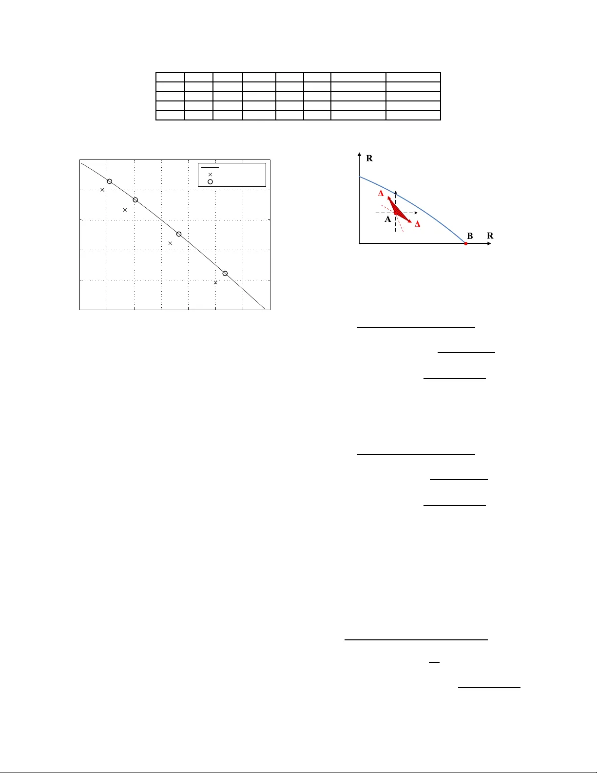
Optimal T ransmission Strategy and Explicit Capacity Region for Br oadcast Z Channels Bike Xie, Studen t Member , IEEE , Miguel Griot, Stude nt Member , IEEE , Andres I. V ila Casado, Stud ent Member , IEEE and Richard D. W esel, S enior Member , IEEE Abstract —This paper pro vides a n ex plicit expression for the capacity re gion of the two-user broadcast Z channel and p ro ves that the optimal boundary can be achieved by independent encoding of each user . Specifically , the inf ormation messages corres pondin g to each user are encoded independen tly and the OR of these two encoded streams i s transmitted. Nonlinear turbo codes that prov ide a controlled distribution of ones and zeros are used to demonstrate a low-complexity scheme th at operates close to the optimal boundary . Index T erms —broadcast chann el, broadcast Z ch annel, capac- ity region, nonli near turb o codes, t urbo codes. I . I N T R O D U C T I O N Degraded bro adcast chann els were first stud ied b y Cover in [1] and a formu lation o f the cap acity region was established in [2], [ 3] and [4]. Sup erposition encoding is the key idea to achieve the o ptimal bound ary of the capacity region for degraded broa dcast channe ls [ 5]. W ith superpo sition en coding for degraded br oadcast channels, the data sent to the user with the mo st degraded channel is enco ded first. Given the encoded b its f or that u ser , an ap propr iate codeb ook f or the second most degraded c hannel user is selected, and so forth. Hence superp osition en coding is, in gene ral, a joint encoding scheme. Howe ver , combin ing indep endently enco ded streams, one for each u ser , is an op timal sch eme for some br oadcast channels including broadcast Gaussian channels [1] and broad- cast binar y-symmetr ic c hannels [1] [2]. Successiv e decodin g is a n atural de coding schem e f or superpo sition encodin g [1] [2] [5]. W ith successive decodin g for d egraded b roadcast chan nels, each receiver first decod es the data sent to the u ser with the most degrad ed chan nel. Conditionin g on th e deco ded d ata for th at user , each rec eiv er determines the code book for th e u ser with the second m ost degraded chann el and decodes that data, an d so fo rth until the desired user’ s data is decod ed. The perfo rmance of successiv e decodin g fo r degrad ed b roadcast chan nels is very clo se to optimal deco ding under normal o perating condition s. T ur bo co des [6] and Low-Density Parity-Ch eck (LDPC) codes [7] perform close to the Shan non limit. LDPC and turbo codin g ap proach fo r b roadcast channe ls wer e studied in [8] and [9] respectively . In [8], LDPC code s provid ed reliable transmission over two-user b roadcast c hannels with additive w hite Gaussian noise (A WGN) an d fading known at the receiver o nly . In [9], a superp osition tu rbo codin g scheme This work was s upported by the Defence Advance d Research Project Agenc y SP A W AR Systems Center , San Diego, Californi a under Grant N66001-02-1-8 938. This paper was presented in part at the Information Theory W orkshop 2007. The authors are with the E lectri cal E ngineer ing Department, Univ ersity of Ca lifornia , Los Angele s, CA 90095 USA (e-mail:xbk@e e.ucla.edu; mgriot@ee .ucla.edu; avila @ee.ucla.ed u; wesel@ee .ucla.edu). X Y 1 1 0 1 a 1 Y 2 0 1 a 2 X Y 1 0 0 1 a ( a ) ( b ) } 0 } Fig. 1. (a) Z channel. (b) Broadcast Z channel . perfor ms within 1dB of th e capacity region boundar y for broadc ast Gaussian channe ls. Both of these app roaches are designed s pecifically for broadcast Gaussian channels and used linear codes. For mu lti-user bin ary a dder channels, n onlinear trellis codes were stu died and d esigned in [1 0]. The Z channel is the binary- asymmetric chann el shown in Fig. 1( a). Th e capac ity of th e Z channel was studied in [11]. Nonlinear trellis codes were d esigned to ma intain a low on es density for the Z channel in [12] [14] and parallel concaten ated nonlinear tur bo cod es were design ed for the Z c hannel in [13]. This paper focuses on th e study of the two-u ser broadcast Z channel X → Y 1 , Y 2 shown in Fig. 1(b). T his pap er p rovides an explicit expression o f the cap acity region fo r the two-user broadc ast Z channel and sho ws that indep endent encodin g with successiv e decodin g c an achieve the boun dary o f this capa city region. This p aper is organize d as follows. Section II in troduce s definitions and notation for br oadcast chan nels. Sectio n III provides the explicit expression of the capa city region for the two-user br oadcast Z ch annel and proves that indepen dent encodin g can achieve the optimal bo undar y of the cap acity region. Section IV presents nonlinea r-turbo co des designed to achiev e the o ptimal bo undar y , and Section V provides the simulation results. Section VI delivers the co nclusions. I I . D E FI N I T I O N S A N D P R E L I M I N A R I E S A. De graded b r oad cast channels The genera l r epresentation of a discrete memoryless broad- cast ch annel is given in Fig. 2. A single signal X is br oadcast to M users thro ugh M different ch annels A 1 , · · · , A M . If p ( y i , y i +1 | x ) = p ( y i | x ) p ( y i +1 | y i ) , th en chan nel A i +1 is a physically degraded version of channel A i (and thus the broadc ast channel X → Y i , Y i +1 is ph ysically degraded ) [5]. A physically degrad ed br oadcast chann el with M users is shown in Fig. 3. Since ea ch u ser decodes its received signal withou t collabo ration, only th e marginal transition probab ilities p ( y 1 | x ) , p ( y 2 | x ) , · · · , p ( y M | x ) of th e co mpon ent channels A 1 , A 2 , · · · , A M affect receiv er performan ce. Hence, the stochastically degraded br oadcast channel is defined in [2] and [5] a s follows: Let A i be a channel with input alphabe t X , o utput alphabet Y i , an d transition prob ability p i ( y i | x ) . Let A i +1 be a nother channel with th e same inpu t alphabet X , output alphabet Y i+1 , and transition pro bability p i +1 ( y i +1 | x ) . A i +1 is a stocha s- tically degraded version of A i if there exists a tr ansition 1 X A 1 A M A 2 .  .  . Y 1 Y 2 Y M Fig. 2. Broadca st channel. A M : p M ( y M | x ) A 2 : p 2 ( y 2 | x ) X A 1 p 1 ( y 1 | x ) D 2 q ( y 2 | y 1 ) Y 1 Y 2 D 3 D M .  .  . Y 3 Y M - 1 Y M Fig. 3. Physical ly degrad ed broadcast channe l. probab ility q ( y i +1 | y i ) such that p i +1 ( y i +1 | x ) = X y i ∈Y i q ( y i +1 | y i ) p i ( y i | x ) . (1) A broa dcast channel with rec eiv ers Y 1 , Y 2 · · · , Y M is a stochastically degra ded bro adcast channel if e very comp onent channel A i is a stochastically degraded version of A i − 1 for all i = 2 , · · · , M [2]. Sin ce the marginal tr ansition pr oba- bilities p ( y 1 | x ) , p ( y 2 | x ) , · · · , p ( y M | x ) completely d etermine a stochastically degrade d broa dcast channe l, we can mod el any stoch astically degrad ed broadc ast channe l as a physically degraded broad cast chann el with the sam e marginal transition probab ilities. Theor em 1 ( [2] [4]): The cap acity region for the two-user stochastically degraded broadca st chann el X → Y 1 → Y 2 is the convex hu ll of the closur e of all ( R 1 , R 2 ) satisfyin g R 2 ≤ I ( X 2 ; Y 2 ) R 1 ≤ I ( X ; Y 1 | X 2 ) , (2) for some joint distribution p ( x 2 ) p ( x | x 2 ) p ( y 1 , y 2 | x ) , where the auxiliary rando m variable X 2 1 has c ardinality boun ded by |X 2 | ≤ min {|X | , |Y 1 | , |Y 2 |} . B. The br oadc ast Z channel The Z channel, shown in Fig . 1(a), is a b inary-asy mmetric channel with th e transition pro bability matrix T =  1 α 0 1 − α  , where 0 ≤ α ≤ 1 . If symb ol 1 is tra nsmitted, symbo l 1 is received with prob ability 1. If sy mbol 0 is tran smitted, symb ol 1 is r eceiv ed with pr obability α an d symbol 0 is rece i ved w ith probab ility 1 − α . W e can mod el the Z c hannel a s th e OR operation o f the chann el in put X and Ber noulli n oise N with parameter α as shown in Fig . 4. In an OR Multiple Access Channel, each u ser appears to transm it over a Z channel when the oth er users are treated as noise [1 3]. Th us, in an OR ne twork with multiple transmitters an d mu ltiple rec eiv ers, each transmitter transmitting to mor e th an one receiver sees 1 U wa s used as the auxiliary random v ariable in [2] [4]. In this paper , we use X 2 instead of U because the auxilia ry rando m vari able corresponds to the second user’ s encoded stream. N Pr ( N = 1) = X Y OR D Fig. 4. OR operation view of Z channel. X Y 1 D 1 Y 2 D ' 1 0 1 0 Fig. 5. Physical ly degraded broadcast Z channe l. a b roadcast Z c hannel if other transmitters transmitting to those receivers are tr eated as no ise. The two-user b roadcast Z chan nel with the marginal transition pro bability matrices T 1 =  1 α 1 0 1 − α 1  T 2 =  1 α 2 0 1 − α 2  is shown in Fig. 1, where 0 ≤ α 1 ≤ α 2 ≤ 1 . Because broadc ast Z channels are stochastically degraded, we can model an y b roadcast Z channel as a physically degraded broadc ast Z channel as shown in Fig. 5, where α ∆ = α 2 − α 1 1 − α 1 . (3) I I I . O P T I M A L T R A N S M I S S I O N S T R A T E G Y F O R T H E T W O - U S E R B RO A D C A S T Z C H A N N E L Since the b roadca st Z chan nel is stocha stically degrad ed, its capacity region can be obtain ed d irectly fro m Theor em 1 . The capacity region for the broadca st Z channel X → Y 1 → Y 2 as shown in Fig. 6 is the conve x hull o f the closu re o f all ( R 1 , R 2 ) satisfying R 2 ≤ I 2 = I ( X 2 ; Y 2 ) = H  ( ¯ µ 2 γ + µ 2 µ 1 )(1 − α 2 )  − ¯ µ 2 H  γ (1 − α 2 )  − µ 2 H  µ 1 (1 − α 2 )  , (4) R 1 ≤ I 1 = I ( X ; Y 1 | X 2 ) = ¯ µ 2  H ( γ (1 − α 1 )) − γ H (1 − α 1 )  + µ 2  H ( µ 1 (1 − α 1 )) − µ 1 H (1 − α 1 )  , (5) for some pr obabilities µ 1 , µ 2 , γ , where µ 1 = Pr ( x = 0 | x 2 = 0) , µ 2 = Pr ( x 2 = 0) , γ = Pr ( x = 0 | x 2 = 1) , H ( · ) is the binary entro py fu nction, ¯ µ 1 = 1 − µ 1 , ¯ µ 2 = 1 − µ 2 and α 2 = Pr { y 2 = 1 | x = 0 } = 1 − (1 − α 1 )(1 − α ∆ ) . (6) Each particular ch oice of ( µ 1 , µ 2 , γ ) in Fig . 6 specifies a particu lar tr ansmission strategy and a rate pair ( I 1 , I 2 ) . The op timal bou ndary of a c apacity region is the set o f all Pareto optimal poin ts ( I 1 , I 2 ) , fo r wh ich it is impo ssible to increase rate I 1 without decrea sing rate I 2 or vice versa. A transmission strategy is optimal if and only if it a chieves a rate p air p oint on the optimal bo undar y . W e call a set X Y 1 D 1 Y 2 D ' X 2 J 2 P 2 P 1 P 1 P Fig. 6. Information theoreti c diagram of the system. of tran smission strategies sufficient if all rate p airs o n the optimal b oundar y can be achieved b y u sing these strategies and time sharing. Further more, a set of transmission strategies is str o ngly sufficient if these strategies can achie ve all rate pairs on the optimal boundary without using time sharing. Equations (4) and (5) give a set of pentago ns th at yield the cap acity region thr ough th eir con vex h ull, b ut do not explicitly sh ow the optimal transmission strategies or derive the b ound ary of the cap acity r egion. A. Optimal transmission strate gies The fo llowing theorem identifies a set of o ptimal trans- mission strategies and provid es an explicit expression of the bound ary o f the capacity r egion. Theor em 2: For a broadcast Z channel with 0 < α 1 < α 2 < 1 , the set o f th e optimal transm ission strategies ( µ 1 , µ 2 , γ ) , which satisfy γ = 0 , (7) 1 (1 − α 1 )( e H (1 − α 1 ) / (1 − α 1 ) + 1) ≤ µ 1 ≤ 1 , (8) and  H ( µ 1 (1 − α 1 )) − µ 1 H (1 − α 1 )  · ln(1 − µ 1 (1 − α 2 )) =  H ( µ 1 (1 − α 2 )) − µ 1 (1 − α 2 ) ln 1 − µ 2 µ 1 (1 − α 2 ) µ 2 µ 1 (1 − α 2 )  · ln(1 − µ 1 (1 − α 1 )) , (9) are strong ly su fficient. In other words, all r ate pairs on the optimal b ound ary of the capacity region can be achiev ed by using exactly th e transmission strategies de scribed in (7-9) without the need of time sharing. Fu rthermo re, applyin g (7 - 9) to (4) and (5) yields an explicit expression of the o ptimal bound ary o f the capacity r egion. Before p roving Theorem 2 , we p resent an d pr ove some preliminar y re sults. Fr om ( 4) and (5), we c an see that the transmission strategies ( µ 1 , µ 2 , γ ) and ( γ , 1 − µ 2 , µ 1 ) have the same transmission rate pairs. T herefor e, we assume γ ≤ µ 1 in the re st of the section without loss o f generality . Theor em 3: For a broadcast Z channel with 0 < α 1 < α 2 < 1 , any transmission stra tegy ( µ 1 , µ 2 , γ ) w ith 0 < µ 2 < 1 , 0 < γ < µ 1 is not op timal. The proo f is giv en in App endix A. Cor ollary 1: The set of all the transmission strategies with γ = 0 is sufficient for any b roadcast Z chann el with 0 < α 1 < α 2 < 1 . Pr oo f: From Theo rem 3, we kn ow that the transmission strategy ( µ 1 , µ 2 , γ ) is op timal on ly if at least one of th ese four equations µ 2 = 0 , µ 2 = 1 , γ = µ 1 , γ = 0 is true. Hence th e set of all th e tr ansmission strategies with µ 2 = 0 , µ 2 = 1 , γ = µ 1 or γ = 0 is sufficient. When µ 2 = 0 , µ 2 = 1 o r γ = µ 1 , the transmission rate for the second user , I 2 in equation (4), is zero. This op timal rate pair is the point B in Fig. 7 (a). Since this point can also be achieved by th e transmission strategy with γ = 0 , µ 2 = 1 and µ 1 = arg max( H ( x (1 − α 1 )) − xH (1 − α 1 )) , all the optima l rate pairs on the optimal b ounda ry of the capacity region c an be ach iev ed by using the transmission strategies with γ = 0 and time sharing. Thus, the s et of all the transmission strategies with γ = 0 is suf ficient. Q.E.D. From Coro llary 1, we can set γ = 0 in Fig. 6 without losing any pa rt of the capac ity regio n an d so the design ed v irtual channel X 2 → X is a Z chan nel. Sinc e we can consider the output of a Z ch annel as the OR operation of two Bern oulli random variables, an independ ent encoding scheme that works well for the bro adcast Z channel will be introdu ced later in this pape r . Applying γ = 0 to ( 4) and ( 5) yields R 2 ≤ I 2 = H ( µ 2 µ 1 (1 − α 2 )) − µ 2 H ( µ 1 (1 − α 2 )) , (10) R 1 ≤ I 1 = µ 2 H ( µ 1 (1 − α 1 )) − µ 2 µ 1 H (1 − α 1 ) . (11) By Cor ollary 1, th e c apacity r egion is the con vex hull of th e closure o f all rate pairs ( R 1 , R 2 ) satisfying (10) and (11) for some proba bility µ 1 , µ 2 . Howe ver , n ot a ll transmission strategies of ( µ 1 , µ 2 , γ = 0) achieve th e op timal bo undary of the capacity region. Since any o ptimal transmission strategy maximizes I 1 + λI 2 for some no nnegative λ , we solve the optimization problem of maximizin g I 1 + λI 2 for any fixed λ ≥ 0 in ord er to find the constrain ts on µ 1 and µ 2 for op timal transmission strategies. Theore m 4 provides the solution to this maximization proble m. Theor em 4: The optimal solution to the maxim ization prob- lem maximize I 1 + λI 2 (12) subject to I 2 = H ( µ 2 µ 1 (1 − α 2 )) − µ 2 H ( µ 1 (1 − α 2 )) I 1 = µ 2 H ( µ 1 (1 − α 1 )) − µ 2 µ 1 H (1 − α 1 ) 0 ≤ µ 2 ≤ 1 , 0 ≤ µ 1 ≤ 1 , is uniqu e an d it is giv en below fo r any fixed λ ≥ 0 . Define ϕ ( x ) = ln(1 − (1 − α 1 ) x ) ln(1 − (1 − α 2 ) x ) (13) and ψ ( x ) = 1 xe H ( x ) /x + x . (14) Case 1: if 0 ≤ λ ≤ ϕ ( ψ (1 − α 1 )) , th en the o ptimal solution is µ ∗ 2 = 1 , µ ∗ 1 = ψ (1 − α 1 ) , wh ich satisfies (8) and (9), and the correspo nding rate pair is I ∗ 1 = H ( µ ∗ 1 (1 − α 1 )) − µ ∗ 1 H (1 − α 1 ) , I ∗ 2 = 0 . Case 2 : if λ ≥ ϕ (1) , th en the op timal solution is µ ∗ 2 = ψ (1 − α 2 ) , µ ∗ 1 = 1 , which also satisfies (8) and (9), and the correspo nding rate p air is I ∗ 1 = 0 , I ∗ 2 = H ( µ ∗ 2 (1 − α 2 )) − µ ∗ 2 H (1 − α 2 ) . Case 3: if ϕ ( ψ (1 − α 1 )) < λ < ϕ (1) , then the optim al solution U p p e r  b o u n d  1 U p p e r  b o u n d  2 ( a ) ( b ) Fig. 7. (a) The capaci ty regi on and two upper bounds. (b) Point Z cannot be on the boundary of the capacit y region. giv en below also satisfies (8) an d (9): µ ∗ 1 = ϕ − 1 ( λ ) = e λ − 1 e λ (1 − α 2 ) − (1 − α 1 ) (15) and  H ( µ ∗ 1 (1 − α 1 )) − µ ∗ 1 H (1 − α 1 )  · ln(1 − µ ∗ 1 (1 − α 2 )) =  H ( µ ∗ 1 (1 − α 2 )) − µ ∗ 1 (1 − α 2 ) ln 1 − µ ∗ 2 µ ∗ 1 (1 − α 2 ) µ ∗ 2 µ ∗ 1 (1 − α 2 )  · ln(1 − µ ∗ 1 (1 − α 1 )) . (16) The pro of is g iv en in Append ix B. Com bining Case 1,2 and 3, we conc lude that ( µ 1 , µ 2 ) is a max imizer of (1 2) if and only if the pair ( µ 1 , µ 2 ) satisfies (8) and (9). In oth er words, if ( µ 1 , µ 2 ) doesn’t satisfy (8) or (9), ( µ 1 , µ 2 ) cannot be a maxim izer of (12), and thus the tra nsmission stra tegy ( µ 1 , µ 2 , γ = 0 ) is not optimal. Since the set of the transmission strategies with γ = 0 is sufficient by Corollary 1, the set of all the transmission strategies satisfying (7-9) is also su fficient. Therefo re th e capacity region is the conv ex h ull of th e closur e of all rate pairs ( R 1 , R 2 ) satisfying (10) and ( 11) for some µ 1 , µ 2 which satisfy ( 8) and ( 9). A sketch of the capacity region is shown w ith two upper bound s in Fig. 7(a) . From Case 1 in T heorem 4, the poin t B correspo nds to the largest tran smission rate fo r the first user . The first up per bound is th e tangent of th e capacity region at the point B , and its slope is − 1 /ϕ ( ψ (1 − α 1 )) . From Case 2, the point A provides the largest tra nsmission rate for the second user . The seco nd uppe r b ound is the tangen t of the capacity region a t the point A , and its slop e is − 1 /ϕ (1) . Case 3 gives us the optimal boun dary o f the capacity r egion except the po ints A and B . Giv en α 1 and α 2 , which completely describe a two-user degraded broadc ast Z ch annel, the op timal b ound ary of the capacity region can b e explicitly d escribed by (8-1 1). For any µ 1 in the range of (8), the value of th e u nique associated µ 2 follows fr om ( 9). The curve of the optimal boundary o f the capacity r egion is then the set o f ( I 1 , I 2 ) pair s satisfying (10) and (11) f or these µ 1 and associated µ 2 . For example, for α 1 = 0 . 15 and α 2 = 0 . 6 , the ran ge of optimal µ 1 values is 0 . 445 ≤ µ 1 ≤ 1 , the rang e of op timal µ 2 values implied by (9) is 0 . 392 ≤ µ 2 ≤ 1 , an d th e associated capacity region bound ary is plotted in Fig. 1 3. Now we prove Theore m 2. Since we ha ve proved tha t the set of all the transmission strategies satisfying ( 7-9) is suf ficient, we only n eed to show that any rate pair o n the optimal X ( W 1 , W 2 ) E n c o d e r Z  c h a n n e l p 1 ( y 1 | x ) D e c o d e r  1 Y 1 1 ˆ w D e c o d e r  2 2 ˆ w Z  c h a n n e l p 2 ( y 2 | x ) Y 2 Fig. 8. Communicat ion system for 2-user broadcast Z channels. W 1 W 2 O R X N 1 O R E n c o d e r  1 E n c o d e r  2 X 1 X 2 Y 1 D e c o d e r  1 1 ˆ w N 1 O R O R N 2 Y 2 D e c o d e r  2 2 ˆ w Fig. 9. Optimal transmission strate gy for broadca st Z channels. bound ary of the capacity region can be achieved without using time sharing. Pr oo f by con tradiction: Su ppose the point Z in Fig. 7(b ) is on the o ptimal b ound ary of the capacity region f or the broadc ast Z channel an d this p oint can o nly b e a chieved by time sharing o f the points X a nd Y , which can be dir ectly achieved by using transmission strategies satisfyin g (7-9). Clearly , the slope of the line segment X Y is neith er zero nor minus infinity . Den ote − k , 0 < k < ∞ a s the slop e of X Y . The points X and Y provide the same value o f I 1 + 1 k I 2 . By Theorem 4, the op timal solution to the m aximization p roblem of max( I 1 + λI 2 ) is u nique, and so neither X no r Y maximizes ( I 1 + 1 k I 2 ) . Thus, ther e exists an achievable p oint P suc h that this po int is o n the righ t up per side of the line X Y . Sin ce and th e tr iangle △ X Y P is in the capac ity region, th e p oint Z must no t be on the op timal bo undary of the capacity region (contrad iction). Q.E.D. B. Indep endent enco ding scheme The commun ication system for th e two-user b roadca st Z channel is shown in Fig. 8. In a general scheme, the tran s- mitter jointly encodes the indep endent messages W 1 and W 2 , which is poten tially to o comp lex to impleme nt. T heorem 2 demonstra tes that there exists an independ ent encoding scheme which achieves th e optim al bound ary o f the cap acity region. Since γ = 0 is stron gly sufficient, the designed cha nnel X 2 → X is a Z cha nnel. Thus, the br oadcast signal X can be constructed as the OR of two Bernoulli rand om variables X 1 and X 2 . T his c onstruction of X is an in depend ent encoding scheme. The system d iagram of the independ ent encod ing scheme is shown in Fig. 9. First th e messages W 1 and W 2 are encod ed separ ately and indepen dently . X 1 and X 2 are two binary random variables with Pr { X j = 1 } = ¯ µ j and Pr { X j = 0 } = µ j , wh ere ¯ µ j + µ j = 1 for j = 1 , 2 . The transmitter br oadcasts X , which is the OR of X 1 and X 2 . From Theo rem 2, this independ ent e ncoding schem e with any choice o f ( µ 1 , µ 2 ) satisfying (8) and (9) achieves a rate pair ( I 1 , I 2 ) arbitrarily c lose to the optimal bo undar y of the capacity region if the codes for X 1 and X 2 are proper ly chosen and have sufficiently large block lengths. Π 1 s 2 s 3 s 4 s 1 u 2 u Look-up table 1 2 3 4 5 6 1 2 1 2 0 n Fig. 10. 16-state nonlinear turbo code structure , with k 0 = 2 input bits per trelli s section. T ABLE I L A B E L I N G F O R C O N S T I T U E N T T R E L L I S C O D E S . R ATE S R 1 = 1 / 6 , R 2 = 1 / 6 . R O W S R E P R E S E N T T H E S TA T E s 1 s 2 s 3 s 4 , C O L U M N S R E P R E S E N T T H E I N P U T u 1 u 2 . L A B E L I N G I N O C TA L N OTA T I O N . User 1 User 2 state input state input 00 0 1 10 11 00 01 10 11 0000 40 20 10 04 0000 07 34 62 51 0001 20 40 04 10 0001 34 07 51 62 0010 10 04 02 01 0010 25 16 43 70 0011 04 10 01 02 0011 16 25 70 43 0100 02 01 40 20 0100 61 13 54 26 0101 01 02 20 40 0101 13 61 26 54 0110 42 21 14 05 0110 23 15 52 64 0111 21 42 05 14 0111 15 23 64 52 1000 01 02 04 10 1000 70 43 16 25 1001 02 01 10 04 1001 43 70 25 16 1010 04 10 20 40 1010 51 62 34 07 1011 10 04 40 20 1011 62 51 07 34 1100 05 14 21 42 1100 64 52 15 23 1101 14 05 42 21 1101 52 64 23 15 1110 20 40 01 02 1110 26 54 13 61 1111 40 20 02 01 1111 54 26 61 13 I V . N O N L I N E A R - T U R B O C O D E S F O R T H E T W O - U S E R B R OA D C A S T Z C H A N N E L In this section we sho w a practical implementation of the transmission strategy fo r th e two-user b roadcast Z channel. As proved in Section III, th e optimal bo undary is achieved by tra nsmitting the OR of the encod ed d ata of each u ser , provided that th e density of ones of each of these encod ed streams is cho sen pro perly . Hence, a family of codes that provides a contro lled de nsity of on es is requir ed. W e use the no nlinear turb o codes, intr oduced in [13], to provide the needed co ntrolled d ensity of ones. No nlinear tur bo co des are parallel concatenated tr ellis codes with k 0 input b its and n 0 output bits per trellis section. A look-u p table assigns the output label for eac h b ranch of the trellis so that the r equired ones de nsity is ach iev ed. Each co nstituent enco der f or th e turbo code in this paper is a 16-state trellis code with k 0 = 2 and the trellis structure sh own in Fig. 10. The o utput labels are assigned via a constrained search that provides the required ones de nsity for each ca se, using the tools presen ted in [1 3] for the Z Channel. The output labels fo r the codes with rate pair ( R 1 = 1 / 6 , R 2 = 1 / 6) , which is simulated on a b roadcast Z chan nel with α 1 = 0 . 15 , α 2 = 0 . 6 , are listed in T able I. Receiv er 1 uses successive decod ing as shown in Fig. 11. Denote as ˆ X 2 the decod ed stream correspo nding to user 2. Since the tran smitted data is x = x 1 ( OR ) x 2 , when ev er a bit x 2 = 1 , there is n o inf ormation abo ut x 1 , and x 1 can b e considered an erasure. Hence, the input stream to Dec oder 1 1 Y e Decoder 2 Decoder 1 1 ˆ X 2 ˆ X 1 Y  Fig. 11. Decoder structure for user 1. 1 0 1 0 e 1 0 0 1 (b) U ser 2: Z ch ann el 2 P (a) Us er 1: Z channel with e rasure s 1 2 1 ( 1 ) P D   1 2 ( 1 ) P D  2 P 2 P 2 1 P D 2 1 ( 1 ) P D  Fig. 12. Percei ved channel by each decoder . is ˆ y 1 = e ( y 1 , ˆ x 2 ) =  y 1 if ˆ x 2 = 0 , e if ˆ x 2 = 1 . (17) Therefo re, Decod er 2 sees a Z Cha nnel with erasures as shown in Fig. 12. The tools p resented in [13] wer e g eneral enoug h to b e app lied to the Z Channel with er asures. N ote that if α 1 is much smaller th an α 2 we can use ha rd decoding in Deco der 2 instead of soft d ecoding witho ut any loss in perfor mance. Since the co de fo r user 2 is desig ned for a Z Channel with 0-to -1 crossover p robab ility 1 − (1 − α 2 ) µ 1 , and the chann el pe rceived by Decoder 2 in user 1 is a Z-Channel with crossover prob ability 1 − (1 − α 1 ) µ 1 < 1 − (1 − α 2 ) µ 1 , the bit error r ate o f ˆ x 2 is negligible comp ared to the bit error rate o f Decoder 1. In fact, in all the simulations shown in Section V, wh ich includ e 100 frame errors of user 1, none of the errors wer e produ ced by Decoder 2. V . R E S U LT S W e simulate the transmission stra tegy fo r the tw o-user broadc ast Z channel with cr ossover pro babilities α 1 = 0 . 15 and α 2 = 0 . 6 , using nonlin ear turb o codes, with the stru cture shown in Fig. 1 0. Fig . 1 3 sho ws the capac ity region for the broadc ast Z chan nel and identifies the simulated rate pairs. It also shows the op timal r ate pairs, which are used to com pute the ones densities of each code. The output labels for the codes with each simulated rate pair are listed at [15]. For eac h of these fou r simulated r ate pairs, the loss in mutu al in formatio n from the associated optimal rate is o nly 0.04 bits or less in R 1 and o nly 0.0 2 bits or less in R 2 . T able II shows bit e rror rates for each rate pair, the ones den sities ¯ µ 1 and ¯ µ 2 , and the in terleaver lengths K 1 and K 2 used for each code. For simplicity , we cho se K 1 and K 2 so that the codeword length n would be the same for user 1 and user 2, except for rate pairs R 1 = 1 / 2 and R 2 = 1 / 22 , w here o ne codew ord length of user 2 is twice the length of user 1 . V I . C O N C L U S I O N S This paper p resented an optim al transmission strategy for the broadcast Z c hannel with independ ent encoding and suc- cessi ve decod ing. W e p roved that any po int on th e optimal T ABLE II B E R F O R T W O - U S E R B R OA D C A S T Z C H A N N E L W I T H C R O S S O V E R P R O B A B I L I T I E S α 1 = 0 . 15 A N D α 2 = 0 . 6 . R 1 R 2 ¯ µ 1 ¯ µ 2 K 1 K 2 BER 1 BER 2 1 / 12 1 / 5 0.106 0.56 4800 1700 2 . 54 × 10 − 5 1 . 24 × 10 − 5 1 / 6 1 / 6 0.196 0.5 2048 2048 7 . 01 × 10 − 6 5 . 33 × 10 − 6 1 / 3 1 / 9 0.336 0.3739 4608 1536 7 . 13 × 10 − 6 6 . 70 × 10 − 6 1 / 2 1 / 22 0.463 0.1979 5632 1024 9 . 27 × 10 − 7 3 . 27 × 10 − 6 0 0.1 0.2 0.3 0.4 0.5 0.6 0.7 0 0.05 0.1 0.15 0.2 0.25 R 1 R 2 Capacity surface simulated rates optimal rates Fig. 13. Broadca st Z channel with crossover probabilitie s α 1 = 0 . 15 and α 2 = 0 . 6 for recei ver 1 and 2 respect iv ely: achie vable capacity region, simulate d rate pairs ( R 1 , R 2 ) and their correspon ding optimal rates. bound ary of the capacity r egion can be achieved by ind e- penden tly encoding the messages cor respond ing to different users and transmitting th e OR o f the encoded signals. Also, the distrib utions of the outpu ts o f each encod er that achieve the optima l bo undary we re provided . Nonlinear-turbo co des that p rovide a controlled d istribution of o nes an d z eros in their codewords were used to demonstrate a l ow-complexity scheme that works close to the optim al b oundar y . A P P E N D I C E S Append ix A Here we p rove Theorem 3, wh ich states that for a broa dcast Z channel with 0 < α 1 < α 2 < 1 , any transmission strategy ( µ 1 , µ 2 , γ ) with 0 < µ 2 < 1 , 0 < γ < µ 1 is not op timal. In (4) an d (5), d enote I 1 ( µ 1 , µ 2 , γ ) = I ( X ; Y 1 | X 2 )   µ 1 ,µ 2 ,γ (18) I 2 ( µ 1 , µ 2 , γ ) = I ( X 2 ; Y 2 )   µ 1 ,µ 2 ,γ (19) I 1 , 2 ( µ 1 , µ 2 , γ ) = ( I 1 , I 2 )   µ 1 ,µ 2 ,γ . (20) The tr ansmission strategy ( µ 1 , µ 2 , γ ) ach iev es the r ate pair I 1 , 2 ( µ 1 , µ 2 , γ ) . Th e theorem is true if we c an increase both I 1 and I 2 when 0 < µ 2 < 1 , 0 < γ < µ 1 . First co mpare the stra tegies ( µ 1 , µ 2 , γ ) an d ( µ 1 + 1 1 2 2 Fig. 14. Capac ity regi on and the changes of rate pairs. ¯ µ 2 δ 1 , µ 2 , γ − µ 2 δ 1 ) for a small positive numbe r δ 1 > 0 . ∆ 1 I 1 = I 1 ( µ 1 + ¯ µ 2 δ 1 , µ 2 , γ − µ 2 δ 1 ) − I 1 ( µ 1 , µ 2 , γ ) ≃ ∂ I 1 ( µ 1 + ¯ µ 2 δ 1 , µ 2 , γ − µ 2 δ 1 ) ∂ δ 1    δ 1 =0 δ 1 = − µ 2 ¯ µ 2 (1 − α 1 ) n ln 1 − γ (1 − α 1 ) γ (1 − α 1 ) + ln µ 1 (1 − α 1 ) 1 − µ 1 (1 − α 1 ) o δ 1 < 0 , (21) and ∆ 1 I 2 = I 2 ( µ 1 + ¯ µ 2 δ 1 , µ 2 , γ − µ 2 δ 1 ) − I 2 ( µ 1 , µ 2 , γ ) ≃ ∂ I 2 ( µ 1 + ¯ µ 2 δ 1 , µ 2 , γ − µ 2 δ 1 ) ∂ δ 1    δ 1 =0 δ 1 = µ 2 ¯ µ 2 (1 − α 2 ) n ln 1 − γ (1 − α 2 ) γ (1 − α 2 ) + ln µ 1 (1 − α 2 ) 1 − µ 1 (1 − α 2 ) o δ 1 > 0 . (22) The small change of th e rate pair (∆ 1 I 1 , ∆ 1 I 2 ) is sho wn Fig. 14. Point A is the rate pa ir of the transmission strategy ( µ 1 , µ 2 , γ ) , the arr ow ∆ 1 shows the small movement of the rate pair (∆ 1 I 1 , ∆ 1 I 2 ) . Second compar e the strategies ( µ 1 , µ 2 , γ ) and ( µ 1 + ( γ − µ 1 ) δ 2 , µ 2 + µ 2 δ 2 , γ ) for a small positive num ber δ 2 > 0 . ∆ 2 I 1 = I 1 ( µ 1 + ( γ − µ 1 ) δ 2 , µ 2 + µ 2 δ 2 , γ ) − I 1 ( µ 1 , µ 2 , γ ) ≃ ∂ I 1 ( µ 1 + ( γ − µ 1 ) δ 2 , µ 2 + µ 2 δ 2 , γ ) ∂ δ 2    δ 2 =0 δ 2 = − µ 2 δ 2 n γ (1 − α 1 ) ln µ 1 γ + (1 − γ (1 − α 1 )) ln 1 − µ 1 (1 − α 1 ) 1 − γ (1 − α 1 ) o = µ 2 δ 2 D ( γ (1 − α 1 ) k µ 1 (1 − α 1 )) > 0 , (23) and ∆ 2 I 2 = I 2 ( µ 1 + ( γ − µ 1 ) δ 2 , µ 2 + µ 2 δ 2 , γ ) − I 2 ( µ 1 , µ 2 , γ ) ≃ ∂ I 2 ( µ 1 + ( γ − µ 1 ) δ 2 , µ 2 + µ 2 δ 2 , γ ) ∂ δ 2    δ 2 =0 δ 2 = µ 2 δ 2 n γ (1 − α 2 ) ln µ 1 γ + (1 − γ (1 − α 2 )) ln 1 − µ 1 (1 − α 2 ) 1 − γ (1 − α 2 ) o = − µ 2 δ 2 D ( γ (1 − α 2 ) k µ 1 (1 − α 2 )) < 0 , (24) where D ( p k q ) is the r elativ e en tropy between the d istri- butions p an d q . The arrow ∆ 2 in Fig. 14 shows the small movement of th e rate pair (∆ 2 I 1 , ∆ 2 I 2 ) . Now we sho w that ∆ 1 I 2 ∆ 1 I 1 < ∆ 2 I 2 ∆ 2 I 1 < 0 . (25) ∆ 1 I 2 ∆ 1 I 1 < ∆ 2 I 2 ∆ 2 I 1 ⇔ D ( γ (1 − α 2 ) k µ 1 (1 − α 2 )) + ln 1 − γ ( 1 − α 2 ) 1 − µ 1 (1 − α 2 ) D ( γ (1 − α 1 ) k µ 1 (1 − α 1 )) + ln 1 − γ ( 1 − α 1 ) 1 − µ 1 (1 − α 1 ) > D ( γ (1 − α 2 ) k µ 1 (1 − α 2 )) D ( γ (1 − α 1 ) k µ 1 (1 − α 1 )) ⇔ D ( γ (1 − α 1 ) k µ 1 (1 − α 1 )) ln 1 − γ ( 1 − α 1 ) 1 − µ 1 (1 − α 1 ) > D ( γ (1 − α 2 ) k µ 1 (1 − α 2 )) ln 1 − γ ( 1 − α 2 ) 1 − µ 1 (1 − α 2 ) ⇔ f ( x ) = D ( γ x k µ 1 x ) ln 1 − γ x 1 − µ 1 x is monotonically increasing i n 0 < x < 1 ⇔ f ′ ( x ) = n ln γ x µ 1 x ln 1 − γ x 1 − µ 1 x −  ln 1 − γ x 1 − µ 1 x  2 + ln γ x µ 1 x  1 1 − γ x − 1 1 − µ 1 x  o γ  ln 1 − γ x 1 − µ 1 x  − 2 > 0 . (26) Let a = 1 − γ x and b = 1 − µ 1 x . W e have 0 < b < a < 1 and want to show that g ( a, b ) = ln a b ln 1 − a 1 − b −  ln a b  2 + ln 1 − a 1 − b  1 a − 1 b  > 0 . (27) Since ∂ 2 g ( a, b ) ∂ a∂ b = − ( a − b ) 2 a 2 b 2 (1 − a )(1 − b ) < 0 , (28) and ∂ g ( a, b ) ∂ a    b = a = 0 ∀ 0 < a < 1 , (29) it is true that ∂ g ( a, b ) ∂ a > 0 ∀ 0 < b < a < 1 . (30) It follows from (3 0) and the fact g ( b, b ) = 0 , ∀ 0 < b < 1 th at g ( a, b ) > 0 , ∀ 0 < b < a < 1 . T hus, the in equality (25) is true, which mean s th at the slop e of ∆ 1 is smaller than th at of ∆ 2 in Fig. 14. Hence, the a chiev able shaded region is on the upper rig ht side of the point A . Theref ore, we can incr ease both terms in th e rate pair I 1 , 2 ( µ 1 , µ 2 , γ ) simultaneou sly an d the strategy ( µ 1 , µ 2 , γ ) is not optimal whe n 0 < µ 2 < 1 and 0 < γ < µ 1 . Q.E.D. Append ix B Here we prove Theorem 4, which p rovides the unique optimal solution to the maximization prob lem (12). In pro blem (12), the objecti ve function I 1 + λI 2 is bounded and the domain 0 ≤ µ 1 , µ 2 ≤ 1 is closed, so th e max imum exists an d can be attained. First we discuss some p ossible op timal solutions and then we show that only o ne of them is op timal fo r any fixed λ ≥ 0 . Case 0: If µ 1 = 0 o r µ 2 = 0 o r µ 1 = µ 2 = 1 , then I 1 = I 2 = 0 and so it cannot be op timal. Case 1: If µ 2 = 1 and 0 < µ 1 < 1 , then I 2 = 0 and ∂ I 1 ∂ µ 1 = (1 − α 1 ) ln 1 − µ 1 (1 − α 1 ) µ 1 (1 − α 1 ) − H (1 − α 1 ) = 0 (31) ⇒ µ ∗ 1 = 1 (1 − α 1 )( e H (1 − α 1 ) / (1 − α 1 ) + 1) . (32) Case 2: If µ 1 = 1 and 0 < µ 2 < 1 , then I 1 = 0 and ∂ I 2 ∂ µ 2 = (1 − α 2 ) ln 1 − µ 2 (1 − α 2 ) µ 2 (1 − α 2 ) − H (1 − α 2 ) = 0 (33) ⇒ µ ∗ 2 = 1 (1 − α 2 )( e H (1 − α 2 ) / (1 − α 2 ) + 1) . (34) Case 3 : If 0 < µ 1 , µ 2 < 1 , th en th e optim um is attained when µ 2 ∂ ( I 1 + λI 2 ) ∂ µ 2 − µ 1 ∂ ( I 1 + λI 2 ) ∂ µ 1 = 0 ⇒ ln (1 − µ ∗ 1 (1 − α 1 )) = λ ln(1 − µ ∗ 1 (1 − α 2 )) , (3 5) and ∂ ( I 1 + λI 2 ) ∂ µ 2 = 0 ⇒ λ  H ( µ ∗ 1 (1 − α 2 )) − µ ∗ 1 (1 − α 2 ) ln 1 − µ ∗ 2 µ ∗ 1 (1 − α 2 ) µ ∗ 2 µ ∗ 1 (1 − α 2 )  =  H ( µ ∗ 1 (1 − α 1 )) − µ ∗ 1 H (1 − α 1 )  ⇒  H ( µ ∗ 1 (1 − α 1 )) − µ ∗ 1 H (1 − α 1 )  · ln(1 − µ ∗ 1 (1 − α 2 )) =  H ( µ ∗ 1 (1 − α 2 )) − µ ∗ 1 (1 − α 2 ) ln 1 − µ ∗ 2 µ ∗ 1 (1 − α 2 ) µ ∗ 2 µ ∗ 1 (1 − α 2 )  · ln(1 − µ ∗ 1 (1 − α 1 )) . (36) For any fixed λ ≥ 0 , the optimal solu tion is in Case 1, 2, or 3. Lemma 1: Functio n ϕ ( x ) = ln(1 − (1 − α 1 ) x ) ln(1 − (1 − α 2 ) x ) is mon otoni- cally increasing in the doma in o f 0 ≤ x ≤ 1 when α 1 < α 2 . Lemma 2: The solution in Case 1 can not be optimal when λ > ϕ ( ψ (1 − α 1 )) . Pr oo f: When µ 2 = 1 and µ 1 = ψ (1 − α 1 ) , ∂ I 2 ∂ µ 1 = 0 and ∂ I 1 ∂ µ 1 = 0 . Ther efore, for any fixed λ , ∂ ( I 1 + λI 2 ) ∂ µ 1 = 0 . When λ = ϕ ( µ 1 ) = ϕ ( ψ (1 − α 1 )) , (35) holds, and so ∂ ( I 1 + λI 2 ) ∂ µ 2    µ 2 =1 ,µ 1 = ψ (1 − α 1 ) = ∂ ( I 1 + ϕ ( ψ (1 − α 1 )) I 2 ) ∂ µ 2    µ 2 =1 ,µ 1 = ψ (1 − α 1 ) = 0 . (37) When λ > ϕ ( ψ (1 − α 1 )) , ∂ ( I 1 + λI 2 ) ∂ µ 2    µ 2 =1 ,µ 1 = ψ (1 − α 1 ) = ∂ I 1 ∂ µ 2    µ 2 =1 ,µ 1 = ψ (1 − α 1 ) + λ ∂ I 2 ∂ µ 2    µ 2 =1 ,µ 1 = ψ (1 − α 1 ) a < ∂ I 1 ∂ µ 2    µ 2 =1 ,µ 1 = ψ (1 − α 1 ) + ϕ ( ψ (1 − α 1 )) ∂ I 2 ∂ µ 2    µ 2 =1 ,µ 1 = ψ (1 − α 1 ) = ∂ ( I 1 + ϕ ( ψ (1 − α 1 )) I 2 ) ∂ µ 2    µ 2 =1 ,µ 1 = ψ (1 − α 1 ) b = 0 , (38) where (a) follows from the facts that ∂ I 2 ∂ µ 2    µ 2 =1 ,µ 1 = ψ (1 − α 1 ) = ln(1 − ψ (1 − α 1 ) · (1 − α 2 )) < 0 and λ > ϕ ( ψ (1 − α 1 )) , and (b) fo llows from (37). Ther efore, Case 1 cann ot be optim al when λ > ϕ ( ψ (1 − α 1 )) . Q.E .D. Lemma 3: The solu tion in Case 2 canno t be op timal wh en λ < ϕ (1) . Pr oo f: When µ 2 = ψ (1 − α 2 ) and µ 1 = 1 , ∂ I 2 ∂ µ 2 = 0 and ∂ I 1 ∂ µ 2 = 0 . Ther efore, for any fixed λ , ∂ ( I 1 + λI 2 ) ∂ µ 2 = 0 . When λ = ϕ ( µ 1 ) = ϕ (1) , (35) holds, a nd so ∂ ( I 1 + λI 2 ) ∂ µ 1    µ 2 = ψ (1 − α 2 ) ,µ 1 =1 = ∂ ( I 1 + ϕ (1) I 2 ) ∂ µ 1    µ 2 = ψ (1 − α 2 ) ,µ 1 =1 = 0 . (39) When λ < ϕ (1) , ∂ ( I 1 + λI 2 ) ∂ µ 1    µ 2 = ψ (1 − α 2 ) ,µ 1 =1 = ∂ I 1 ∂ µ 2    µ 2 = ψ (1 − α 2 ) ,µ 1 =1 + λ ∂ I 2 ∂ µ 2    µ 2 = ψ (1 − α 2 ) ,µ 1 =1 a < ∂ I 1 ∂ µ 2    µ 2 = ψ (1 − α 2 ) ,µ 1 =1 + ϕ (1) ∂ I 2 ∂ µ 2    µ 2 = ψ (1 − α 2 ) ,µ 1 =1 = ∂ ( I 1 + ϕ (1) I 2 ) ∂ µ 1    µ 2 = ψ (1 − α 2 ) ,µ 1 =1 b = 0 , (40) where (a) follows from the facts that ∂ I 2 ∂ µ 1    µ 2 = ψ (1 − α 2 ) ,µ 1 =1 = − ψ (1 − α 2 ) ln α 2 > 0 and λ < ϕ (1) , an d (b) f ollows from (39). Th erefore, Case 2 can not be op timal when λ < ϕ (1) . Q.E.D. Lemma 4: The solution to (3 5) exists in ( 0 , 1) and is uniqu e for any λ in the range of ϕ (0) < λ < ϕ (1) . Pr oo f: Equ ation (3 5) is equiv alent to ϕ ( µ ∗ 1 ) = λ . From Lemma 1, ϕ ( µ 1 ) is monoton ically increasing. Therefore, when ϕ (0) < λ < ϕ (1) , the solu tion µ ∗ 1 is un ique and µ ∗ 1 ∈ (0 , 1) . Q.E.D. Lemma 5: The uniqu e solution ( µ ∗ 1 , µ ∗ 2 ) to (3 5) and ( 36) in Case 3 is optimal if ϕ ( ψ (1 − α 1 )) < λ < ϕ (1) . Pr oo f: Fro m Lemma 4, th e solu tion µ ∗ 1 to (35) is u nique if ϕ ( ψ (1 − α 1 )) < λ < ϕ (1) . From (3 6), m ( µ 2 ) = n H ( µ ∗ 1 (1 − α 2 )) − µ ∗ 1 (1 − α 2 ) ln 1 − µ 2 µ ∗ 1 (1 − α 2 ) µ 2 µ ∗ 1 (1 − α 2 ) o · ln(1 − µ ∗ 1 (1 − α 1 )) − n H ( µ ∗ 1 (1 − α 1 )) − µ ∗ 1 H (1 − α 1 ) o · ln(1 − µ ∗ 1 (1 − α 2 )) = 0 . (41) Clearly , m ( µ 2 ) is m onoto nically incr easing, lim µ 2 → 0 m ( µ 2 ) = −∞ < 0 , (42) and ϕ ( ψ (1 − α 1 )) < λ < ϕ (1) ⇒ µ ∗ 1 > ψ (1 − α 1 ) ⇒ m (1) > 0 . (43) That m eans the un ique solution µ ∗ 2 to (36) is in the d omain of 0 ≤ µ 2 ≤ 1 . Furtherm ore, when ϕ ( ψ (1 − α 1 )) < λ < ϕ (1) , by Lemma 2 and Lemm a 3, Case 1 or Case 2 cann ot be optima l because ∂ ( I 1 + λI 2 ) ∂ µ 2   µ 2 =1 ,µ 1 = ψ (1 − α 1 ) < 0 , (44) ∂ ( I 1 + λI 2 ) ∂ µ 1   µ 1 =1 ,µ 2 = ψ (1 − α 2 ) < 0 . (45) Therefo re, Case 3 is optimal. Q. E.D. Lemma 6: The uniqu e solution ( µ ∗ 2 = 1 , µ ∗ 1 = ψ (1 − α 1 )) in Case 1 is optimal if 0 ≤ λ ≤ ϕ ( ψ (1 − α 1 )) . Pr oo f: When 0 ≤ λ ≤ ϕ ( ψ (1 − α 1 )) , Case 3 is not op timal because there is n o solution µ 1 ∈ (0 , 1) to (35). Case 2 is no t optimal by L emma 3. Hen ce, Case 1 is optimal. Q.E.D. Lemma 7: The uniqu e solution ( µ ∗ 2 = ψ (1 − α 2 ) , µ ∗ 1 = 1) in Case 2 is optimal if λ ≥ ϕ (1) . Pr oo f: When λ ≥ ϕ (1) , Case 3 is not o ptimal b ecause there is no solu tion µ 2 ∈ (0 , 1) to (3 6). Case 1 is not o ptimal by Lemma 2. Hen ce, Case 2 is optimal. Q.E.D. From L emma 5 ,6 a nd 7, Theo rem 4 is immed iately proved. Q.E.D. R E F E R E N C E S [1] T . M. Cov er . Broadcast cha nnels. IEEE T rans. Inform. Theory , IT -18:2– 14, J anuary 1972. [2] P . P . Bergmans. Random coding theorem for broadcast channe ls with degra ded components. IEEE Tr ans. Inform. Theory , IT -19:197–207, March 1973. [3] P . P . Ber gmans. A simple con verse for broadca st channel s with additi ve white Gaussia n noise. IEEE T rans. Inform. Theory , IT -20:279–280, March 1974. [4] R. G. Gallag er . Capacit y and coding for de graded broadcast channel s. Pr obl. P ere d. Inform. , 10:3–14, July–Sept. 1974. [5] T . M. Cove r . Comments on broadcast channels. IE EE T rans. Inform. Theory , 44:2524–25 30, October 1998. [6] C. Berrou, A. Gla vieux and P . T hitimaj shima. Near shannon limit error- correct ing coding and decoding: turbo-c odes. Proc . ICC’93 , pages 873– 890, May 1993. [7] R. G. Gallage r . Low -Density P arity-Che ck Codes . P hD thesis, MIT , Cambridge , MA, 1963. [8] P . Berli n and D. T uninett i. LDPC codes for Gaussian broad cast channels. Signal Proc. Advances in W irele ss Commun., 2004 IE EE 5th W orkshop on , pages 444–448, 2004. [9] T . W . Sun, R. D. W esel, M. R. Shane and K. Jarett. Superposition turbo- TCM for multi-rat e broadcast. IEEE T rans. on Commun. , 52:368–371, 2004. [10] P . R. Che villat . N-user trell is coding for a class of multi ple-acce ss channe ls. IEEE T rans. on Info. Theo. , IT -27:114–120, 1981. [11] S. W . Golomb . The limiting beha vior of the Z-channel. IEEE T rans. Inform. Theory , IT -26:372, May 1980. [12] M. Griot, A. I. Vi la Casado, W -Y . W eng, H. Chan, J. Basak, E. Y ablano vitch, I. V erbauwhe de, B. Jalali and R. D. W esel. Trellis codes with low ones density for the OR multi ple acce ss channel. In IEEE ISIT 2006 , July 2006. [13] M. Griot, A. I. V ila Casado, and R.D. W esel. Non-linea r turbo code s for interl eav er-di vision multiple acc ess on the OR channel. In G LOBECOM ’06. IEEE Global T elecomm. Conf. , 27 Nov . - 1 Dec. 2006. [14] M. Griot, A. I. V ila Casado, W .-Y . W eng, H. Chan and R. D. W esel. Nonlinea r trellis codes for binary-in put bina ry-output multiple access channe ls with s ingle-u ser decoding. Accept ed in IE EE Tr ansaction s on Communicat ions. [15] Nonlinea r turbo codes for broadcast Z channe ls. [Online]. A vailable : http:// www . ee.uc la.edu/ ∼ csl/files/codes/bzc.html . PLA CE PHO TO HERE Bike Xie (S’07) was born in Shanghai, China, in 1983. He recei ved the B.S. degree in electroni c engi- neering from Tsinghua Univ ersity , Beiji ng, China, in 2005, and the M.S. degree in electrica l engineeri ng from Univ ersity of California , Los Angeles, CA, in 2006. He is currently working tow ard the Ph.D. degre e in the Communication Systems Lab at the Departmen t of Electrica l Engineering , Unive rsity of Califor nia, Los Angeles. His research interests are in the area of informati on theory with particular interest in the topics of net- work information theory and channel coding. PLA CE PHO TO HERE Miguel Griot (S’05) recei ved the B.S. degree in elect rical engineering from the Uni versida d de la Re- publica , Uruguay , in 2003, the M.S . and PhD degre e in electri cal enginee ring from the Univ ersity of Cali- fornia at Los Angele s, in 2004 and 2008 respec ti vely . He is currently with Qualcomm Inc., San Die go. His research interests includ e wireless communications, channe l coding, information theory , multiple access channe ls and broadcast channels. PLA CE PHO TO HERE Andres I. Vi la Casado recei ved his B. S. in elec- trical engine ering from the Politecnic o di T orino, T urin, Italy in 2002. He recei ved his M. S. and Ph. D. degrees in ele ctrical engineeri ng from the Uni versit y of California , Los Angeles in 2004 and 2007 respecti vely . At UCLA and at Politec nico di T orino he conduct ed research on communicati on theory with a focus on channe l coding and information theo ry . He is cur - rently a Research Scienti st at Mojix, Inc. where he conduct s researc h on physical layer communications and Bayesia n estimation for RFID applicat ions. PLA CE PHO TO HERE Richard D. W esel is a Professor with the UCLA Electric al Engineeri ng Department and is the Asso- ciate Dean for Academic and Student Aff airs for the UCLA H enry Samueli School of Engineering and Applied Scien ce. He joine d UCLA in 1996 afte r recei ving his Ph.D. in electrical engineeri ng from Stanford. His B.S. and M.S. degree s in electri cal enginee ring are from MIT . His research is in the area of communication theory with particu lar interest in channe l coding. He has recei ved the National Sci- ence Foundation (NSF ) CAREE R A ward, an Oka wa Founda tion award for research in information and telecommuni cations, and the Excellenc e in T eachi ng A ward from the Henry Samueli School of Engineeri ng and Applied Science. He has aut hored or co-author ed ove r a hundred conferenc e and journal publicati ons.