Using Relative Entropy to Find Optimal Approximations: an Application to Simple Fluids
We develop a maximum relative entropy formalism to generate optimal approximations to probability distributions. The central results consist in (a) justifying the use of relative entropy as the uniquely natural criterion to select a preferred approxi…
Authors: ** A. Caticha, R. Preuss (※ 실제 논문 저자는 확인 필요) **
Using Relativ e En trop y to Find Optimal Appro ximations: an Application to Simple Fluids ∗ Chih-Y uan Tseng † Graduate Institute of Systems Biology and Bioinformatics, National Cen tral Univ ersit y , Jhongli 320, T aiwan Ariel Catic ha ‡ Departmen t o f Ph ysics, Univ ersit y at Alban y-SUNY Alban y , NY 12222 USA Abstract W e develo p a maximum relative en tropy forma lism to generate optimal approxima tions to probabilit y distributions. T he cen tral results consist in (a) justifying the use of relative en tropy as the uniquely natural cri terion to s elect a p referred approximatio n f rom within a family o f trial parameterized distributions, and (b) to obtain the optimal app roximation by marginal iz- ing ov er parameters u sing the method of maxim um entrop y and information geometry . As an illustration w e apply our method to simple fluids. The “exact” canonical distribution is approx- imated by that of a fl uid of hard spheres. The proposed method first determines the preferred v alue of the hard-sphere diameter, and then obtains an optimal hard-sphere approximation by a suitably weig hed av erage ov er d ifferent hard-sphere diameters. This leads to a considerable impro vemen t in accounting for the soft-core nature of the in teratomic p otential . As a n umerical demonstration, the radial distribution function and the equation of state for a Lennard-Jones fluid (argon) are compared with results from molecular dy namics simulatio ns. Keywor d : Approximation metho d, Maximum entrop y , Margina lization, Simple fluids, Hard s pher e approximation P A CS : 05.20.Gg, 05.20.Jj 1 In tro duction A common problem in statistical ph ysics is that the pro ba bilit y distribution functions (PDFs) are alwa ys too complicated for practical ca lculations and we need to repla ce them by more tra ctable approximations. A p ossible solution is to iden tify a family of trial distributions { p ( x ) } , where x a re parameters characterized systems and select the member o f the family that is closest to the ex act distribution P ( x ). The problem, of cours e, is that it is not clear what o ne means by ‘closest’. One could minimize Z dx [ p ( x ) − P ( x )] 2 , (1) ∗ Accepted for publication in Ph ysica A, 2008 † He i s cuurently in the transition to Departmen t of Oncology , University of Alb erta, Edmonton AB T6G 1Z2; E-mail: richard617@gmail.com ‡ E-mail: ariel@albany .edu 1 but wh y this particular functional and not another? And also, why li mit oneself to an approximation b y a single member of the trial family? Why not consider a linear combination o f the trial distri- butions, some kind of average over the tria l family? But then, how should we c ho ose the o ptimal weigh t assigned to eac h p ( x )? W e prop ose to tac kle these questions using the metho d of Maxim um relative Entropy (which we abbreviate as ME) and informa tion geometry [1]. The ME metho d, which is develop ed in [2]-[8], has historical ro ots in the ea rlier metho d of maximum entrop y that was pioneered by E. T. J aynes and is co mmonly known as MaxE nt [9]. The ME method is designed for updating probabilities from arbitrary priors for information in the form of a rbitrary constraints and it includes Bay es’ rule and the o lder MaxEnt as sp ecial cases [7], [8]. The purp ose of this pap er is to develop a ME based metho d to generate optimal appr oximations (brief accounts of some of the r esults discussed b elow hav e pr eviously b e en presented in [10] and [1 1]). The general for malism, which is the main result of this paper, is developed in section 2. In section 2.1 we justify the use of r elative entrop y as the unique and natura l criterion to select the preferred approximation, which is lab eled by so me parameters. The optimal approximation is obtained in section 2.2 by mar g inalizing o ver the v ariatio na l par ameters. A suitably w eighed av erag e o ver the whole family of trial distributions with the optimal weight pr ovides an optimal approximation. In the seco nd par t of the paper we demo nstrate the pro po sed formalism b y applying it to s imple classical fluids, a well s tudied field in the past [12]-[15]. T o appr oximate the b ehavior of simple fluids we chose trial distributions that describ e hard spheres [12]-[15] (section 3). The ME formalism is first used (section 4.1) to select the preferred v alue of the hard-sphere diameter. This is equiv alen t to applying the Bogo liub ov v ar iational principle a nd repro duces the re s ults obtained by Manso ori et al. [16] whos e v ar iational principle was justified b y a v ery differe nt argument. An a dv antage of the v ariational or the ME metho ds over the p erturbative appro aches such as Barker and Henders o n (BH) [12] and o f W eeks, Chandler a nd Anderson (W CA) [1 3] is that there is no need for ad ho c criteria dictating how to separa te the int ermolecular p otential into a s trong short r ange repulsio n and a w eak long r a nge attractio n. On the o ther ha nd, a disadv antage of the standard v ariational approach is that it fails to take the softness of the repulsive core int o acco unt . A t high tempera tures this leads to results that a re inferior to the perturba tive approaches. In the standard v a riational a single preferred v alue of the hard-sphere dia meter is selected. But, as discussed in [7] and [17], in the ME metho d non-pr e fer red v alues are not completely ruled out. This allows us (in section 4.2) to mar ginalize over hard s phere dia meter to obtain an optimal har d- sphere a pproximation with a suitable weightin g. Tha t leads to significant improv ements ov er the standard v ariational method. In section 5 we test our metho d by compa r ing its pr edictions for a Lennard- Jones mo del for argon with molecular dynamics simu lation data ([18], [19]). W e find that the ME predictio ns for thermo dynamic v aria bles and for the ra dial distribution function are co nsiderable improv ement s ov er the standard Bo goliub ov v ariational res ult, a nd are compara ble to the pe rturbative results [12] [13]. (F or a recent discuss ion of some of the stre ng ths and limitations of the p erturbative approach see [20].). Despite the shortcomings of perturba tion theor y it remains very p opular b ecause it provides quantit ative insights at a mu ch low er computational cost than dynamical simulations. F or recent applications to the glass transition and o ther more complex s y stems s ee [21] - [25]. Although in this work the ME is not a pplied to such complex pr oblems one may fully exp ect that the information theory based ME metho d will yield insights not o nly the thermo dynamic b ehavior of c o mplex systems but a lso ab out the a ppr oximation methods needed to ana lyze them. Finally , our conclusions and some remarks on further impr ovemen ts are presented in section 6. 2 General formalism of ME optimal appro ximations Consider a sys tem with microstates lab eled by q (for exa mple, the lo cation in phase s pace o r p er haps the v a lues o f spin v ariables). Let the pro bability that the microstate lies within a particular range 2 dq be given by the in tractable canonical distribution P ( q ) dq = e − β H ( q ) Z dq , (2) where Z = R dq e − β H ( q ) def = e − β F is par tition function, in w hich H ( q ) is the Hamiltonian a nd free energy F is defined through this pa rtition function. The goal is to genera te an approximation p ( q ) that is optimal in the sense that is “clos est” to the “exact” distribution P ( q ). It includes tw o steps. The first is to select a pr e ferred trial distribution from a family of trials p ′ ( q | θ ), each member o f the trial family b e ing lab eled by one or mor e parameters θ . More generally , o ne could define the trial family in a non-parametric wa y by sp ecifying v arious constraints. The second is to marginalize ov er parameters θ to o btain an optimal distribution. 2.1 En t ropic criterion for selecting preferred tractable PDFs Relativ e en trop y as the selection criterion. The s election o f the pr eferred approximation is achiev ed by ranking the distributions p ( q ) according to increasing pr efer enc e , a r eal num b er D [ p ] which we call the “entropy” of p . The num be r s D [ p ] are such that if p 1 is prefer red ov er p 2 , then D [ p 1 ] > D [ p 2 ]. Thus, b y design, the “preferr ed” approximation p is that whic h maximizes the ent ropy D [ p ]. Next we determine the functional form of D [ p ]. T his is the g e ner al rule that provides the criterio n for pr e fer ence; in our ca se it defines what w e mea n by the “closes t” or “ preferred” a pproximation. The basic strateg y [3] is one o f induction: (1) if a gener al rule exists, then it mu st apply to spe c ia l cases; (2) if in a certain sp ecial case w e know which is the b es t approximation, then this knowledge can be used to constrain the form of D [ p ]; a nd finally , (3) if enough spec ial cases a re known, then D [ p ] will b e co mpletely determined. The known sp ecia l cases are called the “axioms” of ME a nd they r eflect the co nvicti on that whatever information was origina lly co dified into the e x act P ( q ) is imp ortant a nd should b e pre- served. The selected tria l distribution sho uld coincide with the exact o ne as closely as pos sible and one should only tolerate those minimal c hanges that are demanded b y the information that defines the family of trials. Thr ee axioms and their consequences ar e listed below. Detailed pro ofs and more extensive comments ar e g iven in [7] and [8]. Axiom 1: L o cality . L o c al information has lo c al effe cts. If the co nstraints that define the trial family do not refer to a certain domain D of the v ariable q , then the conditional pr obabilities p ( q | D ) need not b e revised, p ( q | D ) = P ( q | D ). The consequence of the axiom is that non-ov erlapping domains of q co nt ribute additively to the ent ropy: D [ p ] = R dq F ( p ( q )) where F is so me unkno wn function. Axiom 2: Co ordinate in v ariance. The r anking should not dep end on t he system of c o or- dinates. The co ordinates that la b e l the points q are arbitrar y; they car ry no information. The consequence of this axiom is that D [ p ] = R dq p ( q ) f ( p ( q ) / m ( q )) in volves coo rdinate inv ariant s such as dq p ( q ) and p ( q ) /m ( q ), where the function m ( q ) is a densit y , and b oth functions m and f are, at this po int , unkno wn. Next we make a second use of Axiom 1 (lo cality). When there a re no constraints at all a nd the family of trials includes the exact P ( q ) the selected tria l should coincide with P ( q ); that is, the b est approximation to P ( q ) is P ( q ) itself. The conseq uence is that up to nor malization the previously unknown density m ( q ) is the exa ct distribution P ( q ). Axiom 3 : Cons istency for indep endent subsystems . When a syst em is c omp ose d of sub- systems that ar e indep endent it should not matter whether the appr oximation pr o c e dure tr e ats them sep ar ately or jointly. Specifica lly , if q = ( q 1 , q 2 ), and the exact distributions for the subsystems, P 1 ( q 1 ) and P 2 ( q 2 ), are respec tively approximated b y p 1 ( q 1 ) and p 2 ( q 2 ), then the exact distribution for the who le system P 1 ( q 1 ) P 2 ( q 2 ) should be appr oximated by p 1 ( q 1 ) p 2 ( q 2 ). This ax iom restric ts the function f to b e a loga rithm. 3 The ov erall consequence of these axioms is that the trial approximations p ( q ) should be ranked relative to the exact P ( q ) accor ding to their (rela tive) entrop y , D [ p | P ] = − Z dq p ( q ) lo g p ( q ) P ( q ) . (3) The deriv ation has singled out the relative entropy D [ p | P ] a s the unique functional to b e us e d for the purp ose of sele cting a pr eferr e d appr oximation . Other functionals, may b e useful for other purp oses, but they are not a generalization from the simple ca ses described in the axioms ab ove. Remark. Supp ose a mem b er of a family o f trial canonical distributions p ′ ( q | θ ) with Hamiltonian H ( q | θ ) that are conditiona l proba bilit y distr ibutions and dep end on parameters θ = { θ 1 , . . . , θ n } , are giv en b y p ′ ( q | θ ) dq = e − β H ( q | θ ) Z θ dq , (4) where Z θ = R dq e − β H ( q | θ ) def = e − β F θ , in which free energy F θ is also defined. The preferred trial is then selected b y maximizing D [ p ′ | P ]. Substituting Eq. (2) and Eq. (4) int o Eq. (3) gives, D [ p ′ | P ] = β ( h H θ − H i θ − F θ + F ) , (5) where h . . . i θ refers to averages computed with the distribution p ( q | θ ). The inequality D [ p ′ | P ] ≤ 0 , can then be written a s F ≤ F θ + h H − H θ i θ . (6) Thu s, maximizing D [ p ′ | P ] is equiv a lent to minimizing the quantit y F θ + h H − H θ i θ . This form o f the v ariational principle and its use to generate a pproximations is well known. It is usually asso ciated with the name of Bogoliub ov [26] and it is the main technique to generate mean field approximations for discrete systems of spins on a lattice. 2.2 Marginalization for optima l PDF The extent to which the preferre d θ is preferr ed ov er other v alues ([7], [17]) is expr essed by the probability o f θ , p ( θ ). The origina l ME problem of assigning a probability to q is now broadened in to assigning probabilities to b oth q and θ . In this s ection w e use ME again to find the preferred joint distr ibution p J ( q , θ ) = p ( θ ) p ( q | θ ). Note that this is the kind of pr oblem where the Bayesian in terpretation o f proba bilities is esse ntial. Within a frequen tist interpretation it ma kes no sense to talk ab o ut p ( θ ) or ab out p ( q | θ ) b ecause θ is no t a random v ariable; the v a lue of θ is unknown but it is not random. T o pro c e e d we must ask a question. What is the prio r distr ibution, that is, what do we know ab out q and θ b efore the tria l family is specified? The joint pr ior m ( q , θ ) can be expressed acco rding to the pro duct rule as, m ( q , θ ) = m ( q | θ ) m ( θ ), where m ( q | θ ) is conditional probability of obser ving system in state q g iven parameter θ . Our goal is to determine the pr eferred p J ( q , θ ) that is clo sest to the prior m ( q , θ ) that reflects our initial knowledge ab out q a nd ignorance ab o ut the θ s. Initially we know nothing ab out θ , not even ho w it is related to q . The prior that represents this state of knowledge is a pro duct m ( q , θ ) = P ( q ) µ ( θ ) . (7) Indeed, when m ( q , θ ) is a pro duct no correlations b e t ween θ and q are introduced which means that information a bo ut q tells us nothing ab out θ a nd v ice versa. The first factor in m ( q , θ ) reflects our prior knowledge a b o ut q : the distribution for q is known to b e the exact P ( q ). The se c o nd factor reflects our complete ignora nce abo ut θ : we choos e µ ( θ ) to b e as uniform as po ssible. Our method applies whether θ is a dis c r ete or a contin uous v ariable. When θ is a contin uo us v ar iable. 4 Then the uniform distribution µ ( θ ) is such that makes equal volumes in θ space equally lik ely . T o define these volumes we apply metho d of information geometry [1] and note that distances in θ - space ar e uniquely defined b ecause the θ s are la be ls on pro babilit y distributions. Cases wher e θ is a discrete v aria ble are simpler. The r elev ant entropies in volv e sums over θ i rather than integrals and the natural uniform distribution is µ ( θ i ) = constant. In wha t fo llows we concentrate on the more challenging co ntin uous case. The unique dista nce betw een θ and θ + dθ is given by the Fisher-Rao metric [1], dℓ 2 = γ ij dθ i dθ j , where γ ij = Z dq p ( q | θ ) ∂ log p ( q | θ ) ∂ θ i ∂ log p ( q | θ ) ∂ θ j . (8) Accordingly , the volume of a small r egion dθ is γ 1 / 2 ( θ ) dθ , where γ ( θ ) is the determinant of γ ij . Up to a n irrelev ant no rmalization, the distribution µ ( θ ) that is uniform in θ is given by µ ( θ ) = γ 1 / 2 ( θ ). The pre ferred appr oximation p J ( q , θ ) to the joint distribution P ( q ) γ 1 / 2 ( θ ) is then obta ined max- imizing the en tr opy D [ p J | γ 1 / 2 P ] = − Z dq dθ p ( θ ) p θ ( q ) log p ( θ ) p θ ( q ) γ 1 / 2 ( θ ) P ( q ) , (9) b y v arying p ( θ ) sub ject to R dθ p ( θ ) = 1. The final r esult for the pro babilit y that θ lies within the small v olume γ 1 / 2 ( θ ) dθ is p ( θ ) dθ = 1 ζ e D [ p θ | P ] γ 1 / 2 ( θ ) dθ , (10) where D [ p θ | P ] is given in Eq. (5) and ζ is a nor malization constant. Note also that the density exp D [ p θ | P ] is a s c a lar function and the presence o f the Jaco bian factor γ 1 / 2 ( θ ) makes Eq . (10) manifestly inv ariant under changes of the co ordinates θ . Eq. (10) ex pr esses the degr e e to which v alues of θ aw ay from the pre fer red v alue are ruled out; it tells us that the preferred v a lue of θ is that which maximizes the probability density exp D [ p θ | P ]. Finally , now that we hav e deter mined the pr eferred joint distribution p J ( q , θ ) = p ( θ ) p ( q | θ ) we can marginalize θ a nd use the a verage ¯ p ( q ) = Z dθ p ( θ ) p ( q | θ ) (11) as the b est approximation we ca n cons tr uct o ut of the given tria l family . This approximation is exp e cted to b e b etter than a ny individual p ( q | θ ) for the same reason that the mean is exp ected to be a better estimator than the mo de – it minimizes the v ariance. This concludes the first part of o ur pap er. T o s ummarize: our main results co nsist in the justification of the relative en tropy Eq. (3) a s the uniquely natura l functional to selec t the preferr ed approximations and the der iv ation of a quantitativ e measure of the degree to whic h the v arious trials are preferred, Eq. (10). The final result for the b e s t approximation is Eq. (11). Next we illustrate how this ME for ma lism is use d in a specific example: simple fluids. 3 ME optimal hard-sphere appro ximation for simple fluids 3.1 Basic features of simple fluids A simple fluid compo sed of N single atom molecules is describ ed by the Hamiltonian H ( q N ) = N X i =1 p 2 i 2 m + U with U = N X i>j u ( r ij ) , (12) 5 where q N = { p i , r i ; i = 1 , ..., N } a nd the many-bo dy interactions a r e appro ximated b y a pair in teraction, u ( r ij ) wher e r ij = | r i − r j | . The probability that the p o s itions and momenta of the molecules lie within the phase space v olume dq N = 1 N ! h 3 N N Y i =1 d 3 p i d 3 r i (13) is given by canonica l distribution P f ( q N ) dq N = 1 Z f e − β H ( q N ) dq N , (14) where Z f = R dq N e − β H ( q N ) . F or fluids dominated by pair int eractions most thermo dynamic quan- tities of in ter e s t can be wr itten in ter ms of the one- and t wo-particle density distributions n ( r ) = h ˆ n ( r ) i and n (2) ( r 1 , r 2 ) = h ˆ n (2) ( r 1 , r 2 ) i (15) where ˆ n ( r ) = X i δ ( r − r i ) (16) and ˆ n (2) ( r 1 , r 2 ) = X i,j ( i 6 = j ) δ ( r 1 − r i ) δ ( r 2 − r j ) . (17) The t wo-particle correlation function, g ( r 1 , r 2 ) = n (2) ( r 1 , r 2 ) n ( r 1 ) n ( r 2 ) , (18) measures the extent to which the structure o f liquids deviates from complete randomness . If the fluid is homogeneous and isotropic n ( r ) = ρ = N /V and g ( r 1 , r 2 ) = g ( | r 1 − r 2 | ) = g ( r ) wher e ρ is the bulk densit y and g ( r ) is the r adial distribution function (RDF). Then, the pressure is given b y P V N k B T = 1 − β ρ 6 Z d 3 r r du ( r ) dr g ( r ) , (19) where β def = 1 / k B T [12]-[15]. 3.2 Hard-sphere appro ximation T o account for the sho rt-distance repulsion w e consider a family of trials compo sed by distributions that describ e a gas o f hard spheres of diameter r d . F or each r d the Hamiltonian is H hs ( q N | r d ) = N X i =1 p 2 i 2 m + U hs (20) with U hs = N X i>j u hs ( r ij | r d ) , (21) where u hs ( r | r d ) = 0 for r ≥ r d ∞ for r < r d (22) 6 and the corresp onding probability distribution is P hs ( q N | r d ) = 1 Z hs e − β H hs ( q N | r d ) . (23) The partition function and the f ree energy F hs ( T , V , N | r d ) are Z hs = R dq N e − β H hs ( q N | r d ) def = e − β F hs ( T ,V ,N | r d ) . Tw o ob jections tha t can be raised for choos ing P hs ( q N | r d ) as trials are, firs t, that they do no t take the long-rang e int eractions in to account; and second, that the a c tua l short range po ten tial is not that of har d spheres. These are p oints to whic h w e will return la ter. A third ob jection, and this is considerably more serious, is that the exact hard- sphere RDF is not known. How ever, it can be c a lculated within the approximation of P ercus and Y evick (P Y) for whic h there exists an exac t analytical solution ([27], [28], [29]) which is reas onably simple and in go o d ag r eement with numerical sim ulations over a n extended range of temp eratures a nd densities, except p erhaps at high densities. There are several successful pro p osals [30] to improv e up on the PY RDF but they als o represent an a dditional level o f co mplica tion. The simpler PY RDF is sufficien tly accur ate for our current ob j ective – to illustrate the a pplication and study the br oad fea tures of the ME approach. The PY RDF can be wr itten in terms of the La place transform of rg hs ( r | r d ) [29], G ( s ) = ∞ Z 0 dy y g hs ( y r d | r d ) e − sy = sL ( s ) 12 η [ L ( s ) + M ( s ) e s ] , (24) where y is a dimensionless v ariable y = r /r d , L ( s ) = 1 2 η 1 + 1 2 η s + (1 + 2 η ) , (25) M ( s ) = (1 − η ) 2 s 3 + 6 η (1 − η ) s 2 + 18 η 2 s − 12 η (1 + 2 η ) , (26) and η is the packing fraction, η def = 1 6 π ρr 3 d with ρ = N V . (27) The RDF g hs ( r | r d ) is obtained from the in verse transform using residues [3 1]. The equation of state can then b e computed in t wo alternative wa ys, either from the “pressure” equation or from the “compressibilit y” equation but, since the res ult a bove for g hs ( r | r d ) is no t exact, the t wo results do not a gree. It has been found that b etter a greement with simulations and with virial c o efficien ts is obtained tak ing an average of the tw o r esults with weigh ts 1 /3 and 2 /3 resp ectively . The result is the Carnaha n- Starling equation of state, [12]-[15] P V N k B T hs = 1 + η + η 2 − η 3 (1 − η ) 3 . ( 28) The free energy , derived by integrating the equation of state, is F hs ( T , V , N | r d ) = N k B T " − 1 + ln ρ Λ 3 + 4 η − 3 η 2 (1 − η ) 2 # , (29) where Λ = (2 π ~ 2 /mk B T ) 1 / 2 , and the en tropy is D hs = − ∂ F hs ∂ T N ,V = F hs T + 3 2 N k B . (30) It must be remembere d that these expressions are not exa ct. They ar e rea sonable appr oximations for a ll densities up to almo st cry stalline densities (ab out η ≈ 0 . 5). How ever, they fail to predict the face-centered-cubic phase when η is in the range from 0 . 5 up the close-packing v a lue of 0 . 74. 7 4 The M E formalism 4.1 Preferred hard-sphere PDF As discussed in section 2, the trial P hs ( q N | r d ) that is “clos e s t” to the “exact” P f ( q N ) is found b y maximizing the relative ent ropy D [ p | P ], Eq. (3), with p = P hs ( q N | r d ) g iven b y Eq. (23) and P = P f ( q N ) given by Eq . (14). According to Eq. (6), it is equiv alent to minimize F U def = F hs + h U − U hs i hs (31) ov er all diameters r d , where h· · · i hs is computed with P hs ( q N | r d ). Thus, the v ariational approxima- tion to the free energy is F ( T , V , N ) ≈ F U ( T , V , N | r m ) def = min r d F U ( T , V , N | r d ) , (32) where r m is the preferred diameter. T o calcula te F U use h U − U hs i hs = 1 2 Z d 3 rd 3 r ′ n (2) hs ( r , r ′ ) [ u ( r − r ′ ) − u hs ( r − r ′ | r d )] , where n (2) hs ( r , r ′ ) = h ˆ n (2) ( r , r ′ ) i hs . But u hs ( r − r ′ | r d ) = 0 for | r − r ′ | ≥ r d while n (2) hs ( r , r ′ ) = 0 for | r − r ′ | ≤ r d , therefore F U = F hs + h U i hs (33) with h U i hs = 1 2 N ρ Z d 3 r u ( r ) g hs ( r | r d ) , (34) where w e hav e assumed that the fluid is isotropic and homogeneous, n (2) hs ( r , r ′ ) = n (2) hs ( | r − r ′ | ), and in tro duced the hard-sphere RDF g hs ( r | r d ) def = n (2) hs ( r ) ρ 2 . (35) Note that the approximation do es not consist of mere ly replacing the exact free ener g y F by a hard-sphere fre e energ y F hs which neglects the effects of long range attraction; F is approximated b y F U ( r m ) which includes attractio n effects through the h U i hs term in Eq. (33 ). This addre s ses the first o f the t wo ob jections men tioned ea r lier: the real fluid with in ter actions given by u is not b eing replaced by a hard- s phere fluid. The internal energy is approximated b y h H i hs = 3 2 N k B T + h U i hs and not b y h H hs i hs = 3 2 N k B T . T o calcula te h U i hs it is convenien t to write it in terms of V ( s ), the inv erse Laplace transfor m of ru ( r ), y u ( y r d ) = ∞ Z 0 ds V ( s ) e − sy . (36) F or exa mple, for a Lenna r d-Jones po ten tial, u ( r ) = 4 ε σ r 12 − σ r 6 , (37) we hav e V ( s ) = 4 ε " σ r d 12 s 10 10! − σ r d 6 s 4 4! # . (38) 8 Then, using equations Eq. (33) and (24) gives h U i hs = 12 N η ∞ Z 0 ds V ( s ) G ( s ) . (39) Finally , it remains to minimize F U in Eq . (33) to deter mine the preferr ed diameter r m . This is done n umerically in an explicit example for argon in s ection 5. 4.2 Marginalization for optima l hard-sphere PDF The ME metho d a s purs ued in the last section has led us to determine a preferre d ha rd-sphere diameter. It fails to take the s o ftness o f the r epulsive co r e into account. As discussed in section 2.2, our bes t assessment of the distribution of q N is given by the mar ginal o ver r d , ¯ P hs ( q N ) def = Z dr d P J ( q N , r d ) = Z dr d P d ( r d ) P hs ( q N | r d ) . (40) The corresp onding best a ppr oximation to the RDF is obtained us ing Eq. (15), (18), and (35) ¯ g hs ( r ) = Z dq N ¯ P hs ( q N ) ˆ n 2 ( r ) /ρ 2 = Z dr d P d ( r d ) g hs ( r | r d ) . (41) By av erag ing ov er a ll hard-spher e diameters we are effectively descr ibing a soft-core po ten tial. Since ¯ g hs ( r ) takes into account soft-co re effects while g hs ( r | r m ) do es no t, we exp ect that it will lea d to improv ed estimates for all other thermody na mic quan tities. How ever, w e should emphasize that the distribution over the har d- sphere dia meters P d ( r d ) is not being introduced in an a d ho c way in order to “fix” the v ar iational metho d. The in tro duction of P d ( r d ) is mandated b y the ME method (section 2 .2). The distribution of diameters is given by Eq. (10) P d ( r d ) dr d = e D [ P hs | P ] ζ γ 1 / 2 ( r d ) dr d = e − β F U ζ U γ 1 / 2 ( r d ) dr d , (42) where D [ P hs | P ] = β ( F − F U ), the partition functions ζ a nd ζ U are given by ζ = e β F ζ U with ζ U = Z dr d γ 1 / 2 (r d ) e − β F U , (43) and the natural distance dℓ 2 = γ ( r d ) dr 2 d in the space of r d s is given b y the Fisher-Rao metric, γ ( r d ) = Z dq N P hs ( q N | r d ) ∂ log P hs ( q N | r d ) ∂ r d 2 . (44) A conv enient wa y to calculate the Fisher-Rao metric is to expres s it as a seco nd deriv a tiv e of the ent ropy Eq. (3) of p = P hs ( q N | r ′ d ) relative to P = P hs ( q N | r d ), γ ( r d ) = − ∂ 2 ∂ r ′ 2 d D [ P hs ( · | r ′ d ) | P hs ( · | r d ) ] r ′ d = r d , (45) where D [ P hs ( ·| r ′ d ) | P hs ( · | r d )] = β h F hs | r d r ′ d − h U hs | r d r ′ d i r ′ d i , (46) and h· · · i r ′ d is the av er age over P hs ( q N | r ′ d ). As we arg ued ab ove Eq. (33) the exp ectation of the po ten tial ener gy h U hs ( r ′ d ) i r ′ d v anishes b eca use the product u hs ( r | r ′ d ) g hs ( r | r ′ d ) v anishes for b o th r < r ′ d and r > r ′ d . Similarly , h U hs ( r d ) i r ′ d = 0 when r ′ d > r d . How ever, when r ′ d < r d the exp ectation 9 h U hs ( r d ) i r ′ d diverges. The divergence is a consequence of the unphysical nature o f the hard-sphere mo del. F or mor e realistic contin uous p otenti als the distance b etw een r ′ d = r d + dr d and r d is the same as the distance betw ee n r ′ d = r d − dr d and r d . W e can then alw ays choose r ′ d ≥ r d and define γ ( r d ) in Eq. (45) as the limit r ′ d = r d + 0 + . Then, using E q. (29) for F hs , we hav e γ ( r d ) = β ∂ 2 F hs ( r ′ d ) ∂ r ′ 2 d r ′ d = r d +0 + = N π ρr d 4 + 9 η − 4 η 2 (1 − η ) 4 . (47) T o summarize, the distribution o f diameters P d ( r d ) is given by Eq. (42) with F U given by Equations (33), (29), (39) a nd γ given by E q. (47). Our be s t appr oximation to the “ex a ct” P ( q N ) is the ¯ P hs ( q N ) given in Eq. (40). How ever, there is a pro blem. Since the free energ y F U is an extensive quantit y , F U ∝ N , for la r ge N the distribution P d ( r d ) ∼ exp − β F U is very sharply p eaked at the preferred diameter r m . When choosing a single preferr ed diameter for a ma croscopic fluid sample we find that ME confers ov er whelming probability to the preferred v a lue. This is no t surpr is ing. The same thing ha ppe ns when we calculate the global tempera ture or density o f a ma c r oscopic sa mple and yet lo cal fluctuations can b e imp or tant. The q uestion then, is whether lo cal fluctuations are relev ant to the particular quantit ies we want to calculate. W e argue that they a re. F ro m the very definition of g ( r ) as the pr o bability that given an atom at a certain place ano ther atom will b e found at a distance r , it is clear that g ( r ) refers to purely lo cal b ehavior a nd should be influenced b y lo cal fluctuations. T o the extent that the preferred diameter r m depends on temper a ture and density we e x pec t that lo cal temp erature and/or density fluctuatio ns would also induce lo cal diameter fluctuations. F or the purp os e of calculating g ( r ) the system is effectively r educed to the sma ll num b er o f atoms N eff in the lo cal vicinity of the reference ato m at the orig in. In order to develop a systematic, fully ME method for the determination of the effective n umber of particles N eff that are loca lly re le v ant, o ne needs to use trial probability distributions that allow inhomogeneities in the hard spher e diameter s . Y et determination o f such trial probability distributions requires further inv es tig ations. Since we are int erested in demonstra ting ME formalis m for o ptimizing approximations in this work only , w e consider a r ather simple approach to estimate N eff . Based on o ur ME a pproach to a mean field approximation for fluids [10], w e hav e shown the RDF is given by g M F ( r ) = e − β u ( r ) − β ρ R d 3 r ′ u ( r ′ )( g M F ( r − r ′ ) − 1) . (48) F or a sufficient ly dilute g as, the r esults of the mea n field approximation are compar able with ex - per iment al results. The g M F ( r ) is approximately close to the true, exac t RDF g ( R ) for r < σ , the Lennard-Jones para meter. A fluid of hard spher es gives g ( r | r d ) = 0 for r < r d and ca nnot repro duce the b ehavior of E q. (48). Ho wev er, once we reco gnize that we ca n use a statistical mixture, Eq. (40), w e can tune the size N eff of the cell a nd thereb y change the width of P d ( r d ) so that the RDF ¯ g hs ( r ) of E q. (41 ) r epro duces the kno wn short-distance behavior of Eq. (48). 5 Numerical demonstrations: Lennard- Jones “argon” One of the difficulties in tes ting theories ab out fluids aga inst exp erimental data is that it is not ea s y to see whether dis c r epancies ar e to b e blamed to a fa ulty approximation or to a wrong intermolecular po ten tial. This is why theories a r e no rmally tested against mole c ula r dynamics numerical simulations where there is control over the intermolecular p otential. In this section we compar e ME r esults against sim ulation results [1 8] for a fluid of monoato mic molecules interacting through a Lennard- Jones p otential, Eq. (37). The par ameters ε and σ (t he depth of the well, u | min = − ε , and the radius of the repulsive core, u ( σ ) = 0, resp ectively) are c ho sen to model ar gon: ε = 1 . 03 × 10 − 2 eV and σ = 3 . 4 05 ˚ A. 10 5.1 Preliminary examina tions The free energy F U . Figure 1.(A) shows the free energy F U / N k B T as a function of hard-sphere diameter r d for ar gon at a fixed densit y of ρσ 3 = 0 . 65 for different temp e r atures. Figure 1 .(B) shows F U / N k B T as a function of r d for several densities at fixed T = 10 7 . 82 K . Since the critical p oint for argon is a t T c = 15 0 . 69 K and ρ c σ 3 = 0 . 33 a ll these curves, except that at 3 00 K, lie well within the liquid phase. The incr ease of F U / N k B T for high v a lues of r d is due to short r a nge r epulsion b etw ee n the hard spheres describ ed by F hs / N k B T . The increa s e for low r d is due to the L e nna rd-Jones short-ra ng e repulsion as describ ed by h U i hs / N k B T . The pre ferred r d is that which minimizes F U and dep ends b oth on temp era tur e and density . The preferred diameter dec r eases as the temper ature increas es b eca use ato ms with hig her ener gy can penetr a te deeper in to the repulsive core. The dep endence with densit y is less pronounced. The distribution of diameters P d ( r d ) . In section 4.2 we argued that the effective n umber of molecules that is relev a nt to the loc a l structure of the fluid is not the total num b er of molecules in the system N , but a s maller num b er, N eff . In Fig 2.(A) we plo t the distribution o f diameters P d ( r d ) for different temp eratures , fo r a fixed fluid density of ρσ 3 = 0 . 6 5, and for an arbitra rily chosen N eff = 13 5 00. As exp ected the distr ibution shifts to higher diameters as the temperature decreases. Notice also that the distribution beco mes narrower at lower temper atures in ag reement with the fact that a hard-sphere approximation is better a t low T [12]. Figure 2.(B) shows that increa s ing N eff (with fixed density ρ ) decreases the w idth of P d ( r d ) (solid lines) and induces a slight s hift of the who le distribution. This is due to the dep e ndence ∼ ( N eff r d ) 1 / 2 of the Fisher-Ra o measure γ 1 / 2 ( r d ) in 4 7. Figur e 2.(B) also explores the influence of γ 1 / 2 ( r d ) b y comparing the actual distributions P d ( r d ) (solid lines) with the distributions e − β F U ( r d ) (dotted lines) which are o btained by setting γ 1 / 2 = 1 in Eq. (42). The effect of γ 1 / 2 is to shift the distribution sligh tly to higher r d . 5.2 Tw o prop erties of argon The radial di stribution function. W e are finally ready to calculate the r adial distribution g ( r ) for arg on. W e start by estimating the n umber of molecules N eff that are lo cally relev a n t; as explained earlier we choos e N eff so that our bes t approximation ¯ g hs ( r ), Eq. (41), r e pro duces the known short- distance b ehavior g M F ( r ), Eq. (48 ), for r ≪ σ . W e hav e found that the estimates for N eff need not be v ery accurate but that they must b e obta ined fo r ea ch v alue of the temp erature and density . In Fig 3 we show an example of the sho rt-distance behavior of ¯ g hs for three v alues o f N eff at T = 107 . 8 2 K and ρσ 3 = 0 . 65 ; using a Chi-square fit in the range from r = 2 . 9 to 3 . 1 ˚ A the selected b est v alue of N eff is around 38000 . In fig ures 4 .(A)-(D) we compare three different wa ys to calculate the RDF. The so lid line is V erlet’s molecular dyna mics simulation [18]; it pla ys the ro le of exp erimental data ag a inst which we compare our theor y . The dotted line is g hs ( r | r m ) for the hard-sphere fluid with preferred diameter r m . This curve, ca lculated fro m inv erse of Eq. (24), is a ls o the r esult of the v a riational metho d and coincides with the ME result for a macros copically large N eff = N . The dashed line is the av er aged ¯ g hs ( r ) of the extended ME analy sis. Figur es. 4.(A)-(C) were plotted a t three different temp era tures T = 107 . 82, 124 . 11 and 189 . 76 K at the densit y ρσ 3 = 0 . 65. Figure 4.(D) we changed the densit y and the tempera ture to ρσ 3 = 0 . 5 and T = 162 . 93 K . The ag reement betw een the ME curve and V erlet’s data is go o d. The v ast improv ement over the simpler v ariationa l metho d calculation is clear. One might be tempted to dismiss this a chiev ement as due to the a djustmen t of the parameter N eff but this is not quite corr ect: N eff has not b een a djusted, it has b een calculated by fitting ¯ g hs ( r ) to optimal mean field RDF g M F ( r ) for r < σ . Indeed, despite the fact tha t the hard-s phere trial solutions that w e employ are mer e approximations, the funct ional form of the whole cur ve ¯ g hs ( r ) in Eq. (41) is r e pro duced q uite well. How ever, one may note that the agreement b etw e e n the ME prediction and V erlet’s data b eco mes worse when the fluid densit y is decreased or the temp eratur e is incr eased. The re a son has b een sp elled 11 out by in the studies o f WCA [13] They demonstrate that b oth the repulsive and attractive forces contribute to the fluid str uctur e when fluid is a t low and mo derate densities (0 . 4 . ρσ 3 . 0 . 65). How ever, when the fluid density is high enough ( ρσ 3 & 0 . 65), the repulsive force b ecomes dominant. Because the har d-sphere appr oximation do es not include the attra c tive forc e , the hard-sphere RDF do es not take the a ttractive force in to acco un t, and this err or propagates in to our ME pr ediction. The same discrepancy is also revealed in the W CA theory for low densit y [13]. The equation of state. Finally we use the RDF to calculate the equation of sta te from the pressur e equation, Eq. (19 ). In Fig 5 w e compa r e the equation of s ta te derived from the g ( r ) obtained from V erlet’s s im ulation with calculations using the EME and v a r ia tional methods and the per turbative theories of Ba rker a nd Henderson [12] and of W eeks, Chandler and Anderso n [13], at T = 16 1 . 73 K . The EME results constitute a clear improv ement ov er the plain v ariationa l calculation. F or low densities all fo ur metho ds agr ee with each other but differ from the simulation. A b etter ag reement in this reg ion would pro bably require a b etter treatment o f tw o - particle cor relations at long distances. A t int ermediate densities the b est ag r eement is provided by the EME and BH results, while the W CA theory seems to b e the best at high densities. Also shown in Fig 5.(A) ar e exper imental data on arg on [32]. The discrepancy b e tw een the ex per iment al curve and the V e rlet simulation is very likely due to the actual po tential not being pr e c is ely of the Lennar d-Jones t yp e. In Fig 5.(B) w e plo t the EME equation of s tate for three different iso ther ms ( T = 137 . 77, 1 6 1 . 73 and 328 . 2 5 K ). T o co mpare to the simulation of Hansen and V er let [19] we plot β P (rather than β P /ρ ) as a function of densit y ρσ 3 beca use this kind o f plot exhibits the characteristic v an der W aals lo op that signals the liquid-gas transition as the temp erature drops. A more exhaustive explo ration lies, ho wev er , outside the scop e of this pap er. 6 Conclusion The go al of this pap er has b een to use the EME metho d to generate approximations and show that this pr ovides a genera liza tion of the Bogoliub ov v ariational principle. This a ddresses a rang e of applications that lie b eyond the scop e of the traditional MaxEnt. T o test the metho d we co nsidered simple classical fluids. When fac ed with the difficult y of dealing a system described b y a n intractable Hamiltonia n, the traditional approach has b e en to co nsider a s imilar alb eit idealized system describ ed by a simpler more tr actable Ha miltonian. The appro ach w e hav e follow ed here departs from this tr a dition: our goal is no t to identify an approximately similar Hamiltonian but rather to identify an a pproximately similar probability distribution. The end result of the EME approach is a probability distribution which is a sum or an int egral ov er distributions corresp o nding to different har d-sphere diameters. While each term in the sum is of a form that can b e ass o ciated to a real hard-spher e gas, the sum itself is not of the for m exp − β H , and cannot be interpreted a s describing any physical s ystem. As far as the applicatio n to simple fluids is concerned the results a chiev ed in this pap er represe nt progres s but further improv ement s a re p ossible by using better approximations to the har d-sphere fluid and b y choo sing a bro ader family of trial distributions. An imp or tant impro vemen t would be to use trial probability dis tr ibutions that allow inhomogeneities in the hard sphere diameters. This would lead to a systematic, fully EME metho d for the deter mination of the effective num ber of particles N eff that are loca lly relev ant. Many p erturba tive appro aches to fluids ha d b een prop osed, and a gradua l pro cess of selec tio n ov er many years of resear ch led to the optimized theories of BH and WCA. The v a riational ap- proach was definitely less satisfactory than these “b est” perturbation theor ies. With our w o rk, how ever, the s ituation has c hanged: the EME- improv ed v ariational appro ach offers pre dictio ns that already are comp etitive with the b est p ertur ba tive theories. And, of course , the p otential fo r further improv ements of the EME approach rema ins, at this ea rly date, far fr om being ex hausted. 12 Ac kno wledgemen ts The authors ackno wledge R. Scheic her and C.-W. Hong for their v aluable assis tance and advice with the n umerical calculations. References [1] N. N. ˇ Cencov: Statistic al De cision R ules and Optimal Infer enc e, T r ansl. Math. Mono gr aphs, vol. 53 , Am. Math. So c. (Pr ovidence, 1 981);L. L. Campb ell, Proc. Am. Math. So c. 98 (1986 ) 135; for applications to statistics see S. Amari, Differ ential-Ge ometric al Metho ds in Statistics , Springer-V erlag (New Y ork, 19 85); S. Amari and H. Nagaok a, Metho ds of Information Ge ometry , Oxford (Providence, 2000); fo r a brief der iv ation see A. Caticha, Change, time and information geometry , in: A Mohammad-Djafar i (ed), B ay esia n Metho ds and Ma ximu m Entrop y in Science and Engineering , AIP Conf. Pro c. 568 , 2 001 (arXiv:math-ph/000 8018) . [2] J. E. Sho re, R. W. J ohnson, IEEE T rans. Inf. Theory IT-26 (19 8 0) 26; J. E . Sho r e, R. W. Johnson, IEEE T r a ns. Inf. Theory IT-27 (1981) 472. [3] J. Skilling, The Axioms of Ma ximu m Entropy , in: G. J . E ric kson, C. R. Smith (Eds), Maximum- Entrop y and Bay esian Metho ds in Science and Eng ineer ing, Dor dr ech t, Klu wer, 198 8. [4] J. Skilling, Cla s sic Maximum Entrop y , in: J. Skilling (Ed), Ma ximu m Entrop y a nd Bay esian Methods , Dordrech t, Kluw e r , 1 989. [5] J. Skilling, Q uantifi ed Maximum Entrop y , in: P . F. F oug` ere (Ed), Ma x im um Entropy and Bay es ia n Metho ds, Dor drech t, Klu wer, 1990 . [6] I. Csiszar, Ann. Stat. 19 (1991) 2 032. [7] A. Caticha, Relative E ntropy and Inductiv e Inference, in: G. Erickson, Y. Zhai (eds), Bay esian Inference and Maximum Entropy Metho ds in Science and Engineering, AIP Conf. P ro c. 707 , 2004 (arXiv:physics/031109 3 ); A. Caticha and A. Giffin, Up dating Proba bilities, in: K.H. Knuth, A. Caticha, A. Giffin, C. C. Ro dr ig uez, J. L. J . Center (eds.), Bay esian Inference and Maximum En- tropy Metho ds in Science and Engineer ing, AIP Conf. Pro c. 954 , 2007 (ar Xiv:ph ysics/0 6081 8 5 v1 ). [8] A. C a ticha, Lectures on Proba bilit y , Entrop y , and Statistical Ph ysics, in MaxEn08, S˜ ao Paulo, 2008 (arXiv.org/ abs/08 08.00 12); an application to data analysis is given in A. Caticha and R. Preuss, Phys. Rev. E 70 (2004) 04612 71. [9] E. T. Jaynes, Phys. Rev. 1 06 (195 7) 6 20; E . T. Jaynes Phys. Rev. 108 (1957) 171 ; E . T. J aynes in: R D Rosenkr antz (ed), E. T. Jaynes: Pap ers on Pr ob ability, Statistics and St atistic al Physics , Dordrech t (Reidel, 1983); E . T. Jaynes: Pr ob ability The ory: The L o gic of Sci enc e , Ca m bridge Univ ersity P r ess (Cam bridge, 2003). [10] C.-Y. Ts eng, A. Caticha, Maximum Entrop y appr oach to a Mean Field Theory fo r Fluids. in: C. J. Williams (Ed), Bayesian Inference and Maxim um E ntropy Metho ds in Science and Engineering, AIP Conf. Pro c. 659 , 2003 (arXiv:cond-mat/0 2 1219 8 ). [11] C.-Y. Tseng, A. Ca ticha, Maxim um Entrop y Approach to the T heo ry of Simple Fluids, in: G. Erickson and Y. Zhai (E ds), Bay esian Inference a nd Maximum En tropy Metho ds in Science a nd Engineering, AIP Conf. Pro c. 707 , 2004 (arXiv:cond-mat/03 10746 ). [12] J. A. Barker, D. Henderson, Rev. Mo d. Phys. 48 (197 6 ) 58 7. 13 [13] J. D. W eeks, D. Chandler, H. C. Andersen, J. C hem. Phys. 54 (1971) 5237 ; J. D. W eeks, D. Chandler, H. C. Andersen, Science 220 (1983) 787. [14] J. P . Hansen, I. R. McDona ld: The ory of Simple Liquids , 2nd edition, Acad. Press (London, 1986). [15] V. I. Kalikmanov: St atistic al Physics of Fluids , Springer (New Y ork, 200 2). [16] G. A. Manso ori, F. B. Canfield, J. Chem. Ph ys. 5 1 (1969) 4958. [17] Catich a A, Maximum entrop y , fluctuations and priors, in: A Mohammad-Djafari (ed), Bayesian Inference and Maximum Entropy Metho ds in Science and Engineering, AIP Conf. P ro c. 568 , 2001 (arXiv:math-ph/000 8017) . [18] L. V erlet, P h ys. Rev. 165 (1968) 201. [19] J. P . Hansen and L. V erlet, Phys. Rev. 18 4 (1961) 151. [20] P . Ger main and S. Amokrane, Ph ys. Rev. E 65 (20 0 2) 0 3110 91. [21] M. L´ op ez de Haro, M. Robles, Physica A 372 (2006 ) 30 7. [22] C. V aler iani, Z.-J. W ang and D. F renk e l, Mol. Sim. 33 (2007) 1023. [23] T. Urbic, V. lach y , Y u. V. Kalyuzhnji and K. A. Dill, J. Chem. Phys. 1 27 (2007) 174511 . [24] A. B. Adib, Ph ys. Rev. E 75 (2007) 061204. [25] F. F. Beta ncourt-C´ a r denas, L. A. Galicia-Luna and S. I. Sandler, Fluid Phase Equilibria 264 (2008) 174. [26] H. B. Callen: Thermo dynamics and an Int r o duction to Thermo statistics , Wiley (New Y o rk, 1985). [27] J. K. Percus and G. J. Y evick, Ph ys. Rev. 110 (1958) 1. [28] J. K. Percus, Phys. Rev. Lett. 8 (1962 ) 46 2. [29] M. S. W ertheim, P hys. Rev. Lett. 10 (196 3) 321 ; M. S. W er theim, J. Ma th. Phys. 5 (1964) 64 3; E. Thiele, J.Chem. Phys. 39 (1963 ) 47 4. [30] S. Br av o Y us te a nd A. Santos, Phys. Rev. A 43 (199 1) 541 8; S. Br av o Y uste, M. L´ op ez a nd A. Sa nt os, Ph ys. Rev. E 53 (19 96) 48 20-; Y. T ang and B. C.- Y. L u, J. Chem. Phys. 103 (1995) 7463. [31] G. J. Thro op and R. J. Bearman, J. Chem. Ph ys. 4 2 (1965) 2408. [32] J. M. H. Levelt, Physica 26 (1960 ) 36 1. 14 2 . 4 2 . 8 3 . 2 3 . 6 4 . 0 4 . 4 - 8 - 6 - 4 - 2 0 2 4 6 8 1 0 2 . 8 3 . 2 3 . 6 4 . 0 4 . 4 - 3 - 2 - 1 0 1 2 3 4 5 o 3 0 0 o K 1 5 0 o K 1 0 7 . 8 2 o K 6 0 o K F U / N r d ( A ) ( B ) 3 = 0 . 2 3 = 0 . 4 3 = 0 . 6 5 ( A ) Figure 1 : (A): The free energ y F U as a function o f hard-s phere diameter r d for a rgon at a density of ρσ 3 = 0 . 65 for different temp eratures. The b est r d is that which minimizes F U . (B): F U as a function of r d for argon at T = 1 07 . 82 K for differen t densities. 15 2 . 4 2 . 8 3 . 2 3 . 6 4 . 0 4 . 4 0 . 0 0 . 4 0 . 8 1 . 2 1 . 6 2 . 0 2 . 4 2 . 8 3 . 0 3 . 2 3 . 4 3 . 6 3 . 8 4 . 0 4 . 2 0 . 0 0 . 5 1 . 0 1 . 5 2 . 0 2 . 5 3 . 0 3 . 5 6 0 o K 1 0 7 . 8 2 o K 1 5 0 o K 3 0 0 o K P d ( r d ) ( B ) o r d ( A ) 1 / 2 ( r d ) = 1 1 / 2 ( r d ) N e f f = 4 5 0 0 0 N e f f = 3 8 0 0 0 N e f f = 1 9 0 0 0 ( A ) Figure 2: (A): The distribution o f hard-s phere diameters r d for arg on for s e veral temp e r atures at densit y ρσ 3 = 0 . 65 for N eff = 13 5 00. (B): P d ( r d ) for v a rious N eff at T = 1 07 . 82 K and ρσ 3 = 0 . 65. By setting γ 1 / 2 = 1 (dotted lines) we see that the effect of the γ 1 / 2 factor is to cause a slight shift of the distribution. 16 2 . 9 0 2 . 9 5 3 . 0 0 3 . 0 5 3 . 1 0 3 . 1 5 0 . 0 0 0 0 . 0 0 2 0 . 0 0 4 0 . 0 0 6 0 . 0 0 8 0 . 0 1 0 0 . 0 1 2 0 . 0 1 4 0 . 0 1 6 0 . 0 1 8 0 . 0 2 0 e - u ( r ) N e f f = 41000 38000 35000 g ( r ) r ( A ) T = 107.82 o K a nd = 0.65 o Figure 3: Estimating N eff b y requiring that ¯ g hs ( r ) have the corre c t shor t-distance b ehavior e − β u ( r ) . 17 (A) 3 4 5 6 7 8 9 1 0 0 . 0 0 . 5 1 . 0 1 . 5 2 . 0 2 . 5 3 =0 . 6 5 a n d T =1 0 7 . 8 2 o K g ( r ) r ( A ) V e r l e t ' s s i m u l a t i o n M E w i t h N e f f =3 8 0 0 0 H a r d - s p h e r e g ( r ) w i t h r m =3 . 3 9 5 4 A o (B) 3 4 5 6 7 8 9 1 0 0 . 0 0 . 5 1 . 0 1 . 5 2 . 0 2 . 5 3 = 0.65, T = 124.11 o K g ( r ) r ( A ) V e r l e t ' s s i m u l a t i o n M E w i t h N e f f =4 0 0 0 0 H a r d - s p h e r e g ( r ) w i t h r m =3 . 3 7 2 8 A o (C) 3 4 5 6 7 8 9 1 0 0 . 0 0 . 5 1 . 0 1 . 5 2 . 0 2 . 5 3 =0 . 6 5 , T =1 8 9 . 7 6 o K g ( r ) r ( A ) V e r l e t ' s s i m u l a t i o n M E w i t h N e f f =5 0 0 0 0 H a r d - s p h e r e g ( r ) w i t h r m =3 . 3 0 1 6 A o (D) 3 4 5 6 7 8 9 1 0 0 . 0 0 . 5 1 . 0 1 . 5 2 . 0 3 =0 . 5 , T =1 6 2 . 9 3 o K g ( r ) r ( A ) V e r l e t ' s s i m u l a t i o n M E w i t h N e f f =6 2 0 0 0 H a r d - s p h e r e g ( r ) w i t h r m =3 . 3 2 9 5 A o Figure 4: The radial distribution function for (a) the hard-sphere fluid with optimal diameter r m ; (b) V erlet’s mo lec ular dynamics simulation; and (c) the improved E ME analysis , for argon at (A): densit y ρ σ 3 = 0 . 65, temper ature T = 10 7 . 82 K, and effective particle num b er N eff = 38000 . (B): ρσ 3 = 0 . 6 5, T = 1 24 . 11 K, and N eff = 4 0 000. (C): ρσ 3 = 0 . 6 5, T = 189 . 76 K, and N eff = 5 0 000. (D): ρσ 3 = 0 . 5, T = 162 . 93 K, a nd N eff = 6200 0 . 18 0 . 0 0 . 1 0 . 2 0 . 3 0 . 4 0 . 5 0 . 6 0 . 1 0 . 2 0 . 3 0 . 4 0 . 5 0 . 6 0 . 7 0 . 8 0 . 9 1 . 0 1 . 1 1 . 2 0 . 0 0 . 1 0 . 2 0 . 3 0 . 4 0 . 5 0 . 6 0 . 7 0 . 0 0 0 0 . 0 0 5 0 . 0 1 0 P / V e r l e t ' s S i m u l a t i o n M E V a r i a t i o n a l m e t h o d B H t h e o r y W C A t h e o r y L e ve l t ' s e x p e r i m e n t a l d a t a ( B ) P 3 T = 328.25 o K 137.77 o K 1 6 1 . 7 3 o K ( A ) Figure 5: (A): The argon eq uation of state calculated us ing the EME method, the v ariational metho d and the p er turbative theories of BH and W CA a re compa r ed to the V erlet sim ulation at T = 161 . 7 3 K. Also shown are Levelt’s ex p er imen tal results. (B): β P versus the reduced density ρσ 3 calculated using the EME metho d (solid line) and compar e d to the Hansen-V erlet sim ulation for three different isotherms. The g raph shows the app eara nce of the liquid-gas v a n der W aals lo o p as the tempera ture drops. 19
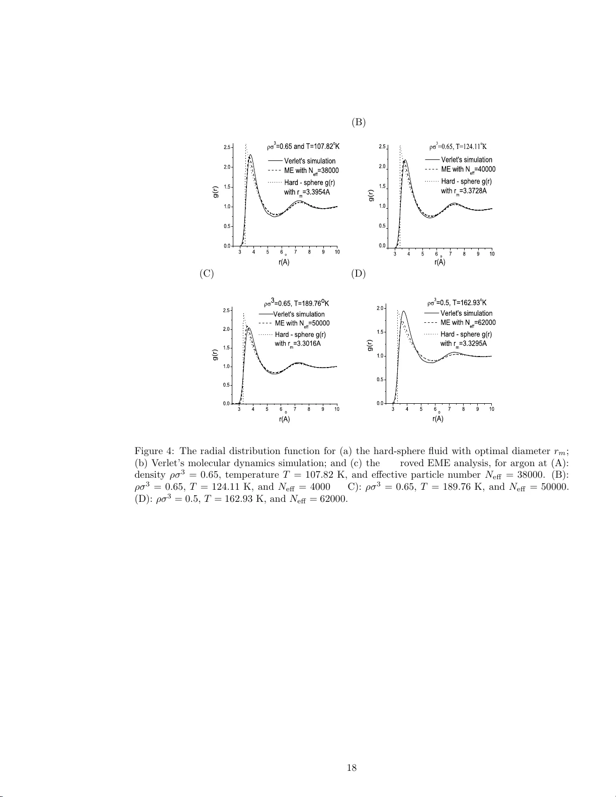
Original Paper
Loading high-quality paper...
Comments & Academic Discussion
Loading comments...
Leave a Comment