Error Exponents of Optimum Decoding for the Interference Channel

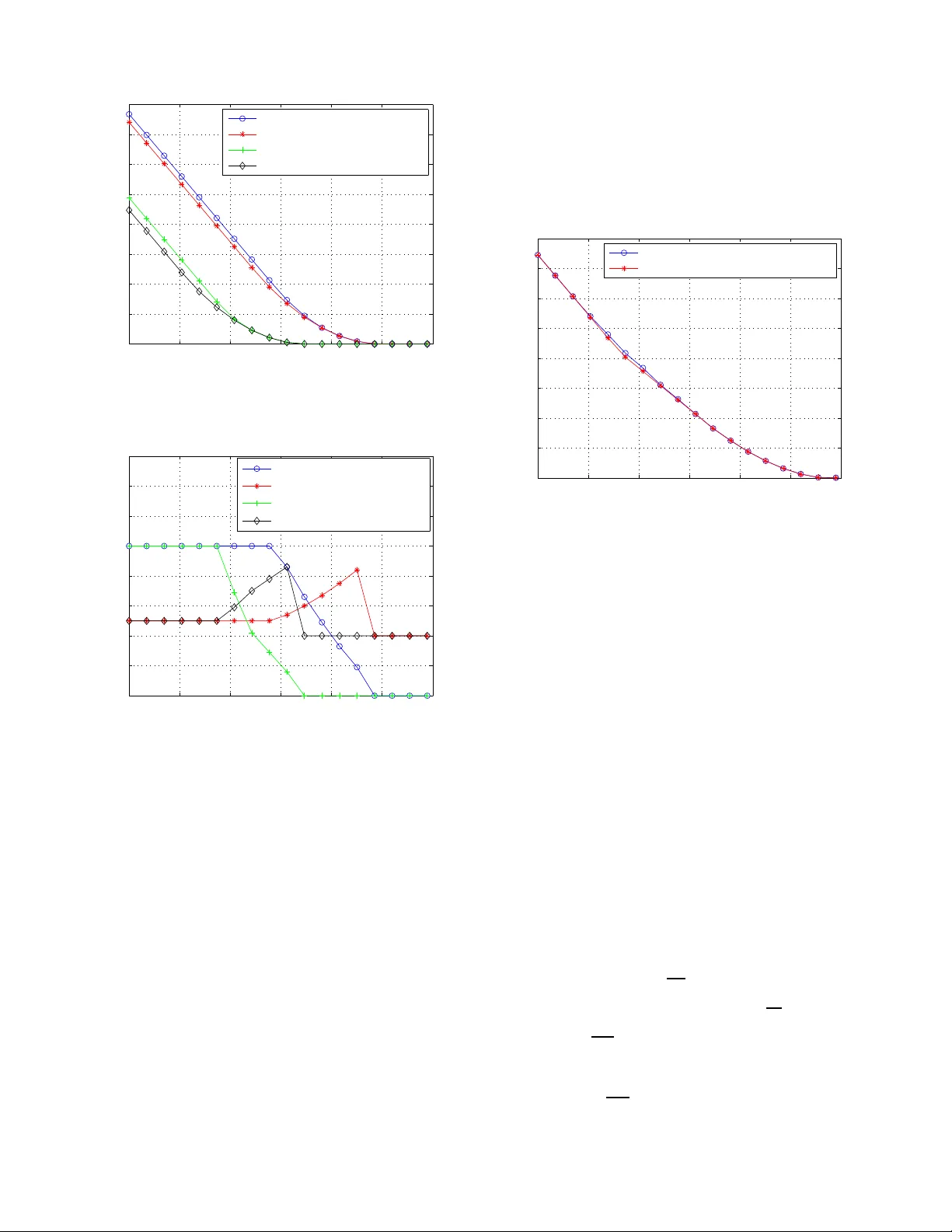
1 Error Exponents of Optimum Decoding for the Interfer ence Channel Raul H. Etkin † , Member , IEEE, Neri Merhav ‡ , F ellow , IEEE, and Erik Ordentlich † , Senior Member , IEEE raul.etkin@hp.com, merhav@ee.technion .ac.il, erik.ordentlich@hp.co m Abstract —Exponential error bounds f or the finite–alphabet interference chann el (IFC) with t wo transmitt er –r eceiv er pairs, are inv estigated under th e random coding regime. Ou r focus is on optimum decoding, as opposed to heuristic d ecoding rules that hav e been used in prev ious works, like joint typicality decoding, decoding based on in terference cancellation, and d ecoding that considers the interference as addit ional noise. Indeed, the fact that the actual interfering signal is a codew ord and not an i.i.d. noise process complicates the application of conv entional techniques to the performance analysis of the optimum d ecoder . Using analytical tools rooted in statisti cal physics, we derive a single letter expression f or error exponents achievable under optimum decoding and demonstrate st rict improv ement over error exponents obtainabl e using suboptimal decoding rules, but which ar e amenable to more conv entional analysis. Index T erms —Error exponen t region, large d eviations, method of types, statistical physics. I . I N T RO D U C T I O N The M -user interferen ce ch annel (IFC) mod els th e commu - nication between M transmitter-receiver pairs, wher ein each receiver must decode its correspo nding tr ansmitter’ s message from a signal that is c orrup ted by interferen ce from the other transmitters, in add ition to channel noise. Th e info rmation theoretic analysis of the IFC was initiated over 30 year ago and has recently witnessed a resurgen ce of inter est, m otiv ated by new potential applications, such as wireless com munication over unregulate d spectrum . Previous work on the IFC has focused on ob taining in ner and outer boun ds to the capacity region for memory less interferen ce an d noise, with a precise ch aracterization of the capacity region rem aining elusi ve for most channels, even for M = 2 users. The best k nown inner bound for the IFC is the Han-Kobayashi (HK) region, established in [1]. It has b een found to be tight in certain special cases ([1], [2]), and recen tly was f ound to be tigh t to within 1 bit for the two user Gau ssian IFC [ 3]. No achievable rates th at lie outside the HK region a re known for any IFC with M = 2 users. Our aim in this paper is to extend the study of achiev able schemes to the analy sis of error exponents, or exponential rates of d ecay of erro r prob abilities, th at are attainab le as a function o f u ser r ates. T o o ur k nowledge, th ere h as b een no prior treatment of error expon ents for the IFC. In particu lar , † R. Etkin and E. Ordentl ich are with Hewlet t-Pa ckard Laboratories, Palo Alto, CA 94304, USA. ‡ N. Merh av is wit h T echnion - Israel Institu te of T echnol ogy , Haifa 32000, Israel. Part of this work was done while N. Merha v was visitin g Hewle tt– Pack ard Laboratories in the Summers of 2007 and 2008. the er ror b ounds und erlying the achiev ability results in [ 1] yield vanishing error expo nents (thoug h still decaying error probab ility) at all rate s. The n otion of an error exponent r egion, or a set of achiev- able exponential rate s of d ecay in the error prob abilities for different users at a g i ven o perating rate-tuple in a multi-user commun ication ne twork, was formalized recently in [4], and studied therein for Gaussian mu ltiple access and bro adcast channels. Ou r ma in result, presented in Section IV, is a single letter characterizatio n of an ach iev ab le error expo nent region, as a function of user rates, for the M = 2 user finite alphab et, memory less interf erence ch annel. T he region is deriv ed by bound ing the a verage error pr obability of ran dom c odeboo ks comprised of i.i.d. codewords unifor mly distrib u ted over a type class, u nder maximu m likelihood (ML) decod ing a t ea ch user . Unlike the single user setti ng, in th is case, the effective channel determinin g each receiver’ s ML decoding ru le is in duced both by the noise and the interf ering user’ s codebo ok. Our focu s on op timal d ecoding is a departu re fro m th e co n ventional achiev ability argu ments in [1] and elsewhere, which are b ased on joint-typ icality d ecoding , with restrictions on the decoder to “trea t in terferenc e as noise” or to “decod e the interferen ce” in part o r in whole . Howe ver , in this work, we co nfine our analysis to codeb ook ensemb les that are simpler than the superpo sition codeb ooks of [1]. The analysis of the p robab ility of decod ing error un der optimal d ecoding is complicated due to corr elations induced by the interferin g signal. Usual metho ds for bou nding the probab ility o f e rror b ased o n Jensen’ s ine quality an d other related inequ alities (see, e.g. , (8) below) fail to give go od results. Our bou nding appro ach combines some of the clas- sical information theore tic appro aches of [5] and [6] with a n analytical techniq ue f rom statistical phy sics th at was app lied recently to the stu dy of single u ser ch annels in [7], [8]. More specifically , as in [5], we u se auxiliary para meters ρ a nd λ to ge t an u pper bo und on th e average probability of decodin g error und er ML d ecoding , which we then bound usin g th e method of types [6]. Ke y in our deriv ation is th e use o f distance e numerato rs in th e sp irit of [7] and [8], which allows us to av oid using Jensen’ s inequality in some steps, an d allows us to mainta in exponential tightness in othe r inequalities by applying them to only polyn omially few terms (as opposed to exponentially many) in certain sums that b ound the pro bability of decoding error . It should be emphasized, i n this context, that the use of th is tec hnique was p iv o tal to our results. Our earlier attempts, th at were b ased on more ‘traditional’ to ols, failed to provide meaningf ul results. I n fact, they all turn ed out to be 2 inferior to some trivial b ound s. The paper is organ ized as follows. The notation, various definitions, a nd the channe l mo del assumed through out the paper are detailed in Sectio n II. In Sectio n III, we d eriv e an “easy” set o f attainable err or exponents which we shall treat as a benchmark for the e xponents of the main section, Section IV. The “easy ” exponen ts are o btained by simp le extensions to the interferen ce channe l of existing err or expo nent results for single user and multiple access chann els, based on ran dom constant compo sition codeb ooks and subo ptimal d ecoders. Then, in Section IV, we derive anothe r set o f attainable exponents by analyzin g ML decodin g for the channel ind uced by the interfer ing codeboo k. In Section V, we show that the minimization s require d to e valuate the ne w error exponen ts can be wr itten as conv ex optim ization pr oblems, and, as a result, can be solved e fficiently . W e follow this up in Section VI with a numerical comp arison o f t he ne w expo nents with the baseline exponents of Sectio n III f or a simple IFC. These n umerical results d emonstrate that the new exponents are never worse (at least for the cho sen ch annel and par ameters) and , fo r most rates, strictly improve over the baseline exponents. An earlier version of this work was presented in [9]. I I . N O TA T I O N , D E FI N I T I O N S , A N D C H A N N E L M O D E L Unless otherwise stated, we use lowercase a nd u ppercase letters f or scalar s, b oldface lowercase letters for vecto rs, upperc ase (bo ldface) letters for ran dom variables ( vectors), and calligrap hic letters for sets. For example, a is a scalar , v is a vector, X is a random variable, X is a rando m vector , and S is a set. For a real numb er a we shall, on occasion , let a denote 1 − a . Also, we use log ( · ) to denote natu ral logar ithm, E to d enote expectation , and Pr to d enote prob ability . For in depend ent ran dom variables X and Y d istributed according to P X,Y ( x, y ) = P X ( x ) P Y ( y ) , ( x, y ) ∈ X × Y , we denote the conditional e xpectation operator E X ( · ) as E X ( f ( X , Y )) △ = P x ∈X f ( x, Y ) P X ( x ) for any function f ( · , · ) . All inform ation quantities (entr opy , mu tual informa tion, etc.) an d rates are in nats. Finally , we use . = , . ≤ , etc., to d enote equality or ineq uality to the first o rder in the expo nent, i. e. a n . = b n ⇔ lim n →∞ 1 n log a n b n = 0 ; a n . ≤ b n ⇔ lim sup n →∞ 1 n log a n b n ≤ 0 . The empirical probability mass fu nction of the finite al- phabet seque nce v = ( v (1) , . . . , v ( n )) with alphabet V is denoted as the vector { P v ( v ) , v ∈ V } , where each P v ( v ) is th e relative f requen cy of v ( i ) = v alon g v . The type class associated with an emp irical prob ability mass fun ction P , which will be denoted by T P , is the set o f all n –vectors { v } wh ose empirical pro bability mass functio n is equal to P . Similar co n ventions will app ly to pairs and triples of vectors of leng th n , wh ich are de fined over the cor respond ing prod - uct alpha bets. Inf ormation m easures pertain ing to empirical distributions will be deno ted using the standard notatio nal conv entions, except that we u se “ ˆ ” as well as subscr ipts that indicate the seq uences fr om which these empirical distribu- tions were extracted. For example, we write ˆ H xy z ( X, Y | Z ) and ˆ I xy z ( X, Y ; Z ) to denote the conditio nal entropy of ( X, Y ) given Z and the mutu al inf ormation b etween ( X, Y ) and Z , respe cti vely , comp uted with respect to the e mpirical distribution P xy z ( x, y , z ) . W e den ote the relative en tropy or Kullback -Leibler div ergence between d istributions P X and P Y as D ( P X || P Y ) △ = P x P X ( x ) log( P X ( x ) /P Y ( x )) , and we write D ( P X | Z || P Y | Z | P Z ) for the con ditional relativ e entropy betwee n con ditional distributions P X | Z and P Y | Z condition ed on P Z , whic h is de fined as D ( P X | Z || P Y | Z | P Z ) △ = P x,z P Z ( z ) P X | Z ( x | z ) lo g( P X | Z ( x | z ) /P Y | Z ( x | z )) . W e continu e with a formal d escription of the two–user IFC setting. Let x i = ( x i (1) , . . . , x i ( n )) ∈ X n i , i = 1 , 2 , denote the channel input signals of the two tran smitters, an d let y i = ( y i (1) , . . . , y i ( n )) ∈ Y n i be the cor respond ing channel outp uts received by deco ders 1 and 2, where X i and Y i denote th e input and ou tput alphabets, a nd which we assume to be finite. Each (rando m) outpu t symb ol pair ( Y 1 ( j ) , Y 2 ( j )) is assumed to be conditiona lly indep endent of all o ther ou tputs, and all input symbo ls, giv en the two correspo nding (r andom) input symb ols ( X 1 ( j ) , X 2 ( j )) , an d the correspo nding con ditional probab ility is assumed to be constant from symbo l to symbol. An ( n, R 1 , R 2 ) code for the IFC co nsists of pairs o f encoding and d ecoding function s, ( f 1 , f 2 ) and ( g 1 , g 2 ) , respectiv ely , where f i : { 1 , . . . , M i } → X n i , M i = ⌈ e nR i ⌉ , and g i : Y n i → { 1 , . . . , M i } , i = 1 , 2 . The per forman ce o f th e code is character ized by a pair of error proba bilities P e,i = Pr ( ˆ W i 6 = W i ) , i = 1 , 2 , wh ere ˆ W i = g i ( Y i ) and Y i is the rand om ou tput when user i transmits X i = f i ( W i ) , assuming the messages W i are unifor mly distributed o n the sets of indices { 1 , 2 , . . . , M i } , i = 1 , 2 . The p er user erro r p robabilities d epend on the channel only th rough th e ma rginal cond itional distributions of the channel outpu ts given the correspo nding chann el in- put p airs. W e shall denote the se co nditional distributions a s q i ( y | x 1 , x 2 ) △ = Pr ( Y i ( j ) = y | ( X 1 ( j ) , X 2 ( j )) = ( x 1 , x 2 )) . A pair of er ror expon ents ( E 1 , E 2 ) is attainable at a rate pair ( R 1 , R 2 ) if the re is a seq uence of ( n, R 1 , R 2 ) cod es satisfying E i ≤ lim inf n →∞ − (1 /n ) lo g P e,i for i = 1 , 2 . The set o f all attaina ble er ror exponents at ( R 1 , R 2 ) co mprises th e error exponen t region at ( R 1 , R 2 ) and we shall denote it as E ( R 1 , R 2 ) . Th e main result o f this paper is a single letter characterizatio n o f a no n–trivial subset of E ( R 1 , R 2 ) for each R 1 , R 2 . I I I . B A C K G RO U N D In this section, we p resent achievable erro r exponents for the inte rference chan nel which are b ased o n kn own results of error expon ents fo r single user and multiple access ch annels (MA C) f or fixed composition codeb ooks [12], [13], [11]. These exponen ts will b e used as a baseline for c omparin g the perfor mance of the error expo nents that we derive in Sectio n IV. In the following, we will focus on the error performan ce o f user 1, and a s a r esult, all explana tions an d expressions will be specialized to receiver 1. Similar expr essions also hold for user 2 with the exchan ge of indic es 1 ↔ 2 . 3 A po ssibly suboptimal decode r for the interf erence channel can b e ob tained fro m a giv en multiple access chan nel decod er by simply ignoring th e de coded message of the interfering transmitter . For example, following [13], we can use a mini- mum en tropy decod er that f or a given receiv ed vector y 1 at receiver 1 comp utes ( ˆ x 1 , ˆ x 2 ) ( ˆ x 1 , ˆ x 2 ) = arg min ( ˜ x 1 , ˜ x 2 ) ∈C 1 ×C 2 ˆ H ˜ x 1 ˜ x 2 y 1 ( X 1 , X 2 | Y 1 ) , and throws away ˆ x 2 . It f ollows from [13] that for rand om codeb ooks of fixed composition Q 1 , Q 2 , the average pro bability of decodin g both messages in erro r , where the averaging is done over the random choice of co deboo ks, satisfies: Pr( ˆ x 1 6 = x 1 , ˆ x 2 6 = x 2 ) . ≤ e − nE 1 , 2 where E 1 , 2 = min P ˆ X 1 ˆ X 2 ˆ Y 1 : P ˆ X 1 = Q 1 ,P ˆ X 2 = Q 2 D ( P ˆ Y 1 | ˆ X 1 ˆ X 2 || q 1 | P ˆ X 1 , ˆ X 2 ) + I ( ˆ X 1 ; ˆ X 2 ) + | I ( ˆ X 1 ; ˆ Y 1 ) + I ( ˆ X 2 ; ˆ X 1 , ˆ Y 1 ) − R 1 − R 2 | + with | · | + = max {· , 0 } . In addition, the average probability of decodin g t he message of the interferin g transmitter cor rectly but the message of the desired transmitter inco rrectly satisfies: Pr( ˆ x 1 6 = x 1 , ˆ x 2 = x 2 ) . ≤ e − nE 1 | 2 where E 1 | 2 = min P ˆ X 1 ˆ X 2 ˆ Y 1 : P ˆ X 1 = Q 1 ,P ˆ X 2 = Q 2 D ( P ˆ Y 1 | ˆ X 1 ˆ X 2 || q 1 | P ˆ X 1 , ˆ X 2 ) + I ( ˆ X 1 ; ˆ X 2 ) + | I ( ˆ X 1 ; ˆ X 2 , ˆ Y 1 ) − R 1 | + . Therefo re, th e overall average e rror pe rforman ce o f this MAC decoder in the IFC satisfies: Pr( ˆ x 1 6 = x 1 ) . ≤ e − n min { E 1 , 2 ,E 1 | 2 } . A second subo ptimal decod er that leads to tractab le error perfor mance boun ds is the single user maximu m mutual informa tion dec oder ( which in this case coincides with the minimum entropy decoder ): ˆ x 1 = arg max x 1 ∈C 1 ˆ I x 1 y 1 ( X 1 ; Y 1 ) . In this case, standard application of the method of types [11] leads to the fo llowing boun d on th e a verage e rror pro bability under rando m fixed comp osition cod ebook s of types Q 1 , Q 2 : Pr( ˆ x 1 6 = x 1 ) . ≤ e − nE 1 , where E 1 = min P ˆ X 1 ˆ X 2 ˆ Y 1 : P ˆ X 1 = Q 1 ,P ˆ X 2 = Q 2 D ( P ˆ Y 1 | ˆ X 1 ˆ X 2 || q 1 | P ˆ X 1 , ˆ X 2 ) + I ( ˆ X 1 ; ˆ X 2 ) + | I ( ˆ X 1 ; ˆ Y 1 ) − R 1 | + . W e can cho ose th e better decoder between these two, that leads to the be tter er ror p erform ance. There fore, we o btain that E B , 1 = max { E 1 ; min { E 1 , 2 ; E 1 | 2 }} (1) is an achiev able erro r exponent at receiver 1, with an analogou s exponent fo llowing for receiver 2. I V . M A I N R E S U LT Our main con tribution is stated in the following th eorem, which presents a new error exponent region for th e discrete memory less two–user IFC. While the full pro of appear s in Append ix A, we also provide a proof outlin e below , to give an idea of the main steps. Theor em 1: For a d iscrete m emoryless two-user I FC as defined in Section I, for a family of block codes o f rates R 1 and R 2 a decod ing erro r probab ility for user 1 satisfyin g lim inf n →∞ − 1 n log P e, 1 ( n ) ≥ E R, 1 ( R 1 , R 2 , Q 1 , Q 2 , ρ, λ ) (2) can be achieved as th e block length of th e codes n goes to infinity , wh ere the error exponent E R, 1 ( R 1 , R 2 , Q 1 , Q 2 , ρ, λ ) is giv en b y E R, 1 ( R 1 , R 2 , Q 1 , Q 2 , ρ, λ ) = ( R 2 − ρR 1 + min ( min ( P ˆ X 1 ˆ X 2 ˆ Y 1 ,P ˆ X ′ 1 ˆ X ′ 2 ˆ Y ′ 1 ) ∈S 1 ( Q 1 ,Q 2 ) f 1  ρ, λ, P ˆ X 1 ˆ X 2 ˆ Y 1 , P ˆ X ′ 1 ˆ X ′ 2 ˆ Y ′ 1  ; min ( P ˆ X 1 ˆ X 2 ˆ Y 1 ,P ˆ X ′ 1 ˆ X ′ 2 ˆ Y ′ 1 ) ∈S 2 ( Q 1 ,Q 2 ,R 2 ) f 2  ρ, λ, P ˆ X 1 ˆ X 2 ˆ Y 1 , P ˆ X ′ 1 ˆ X ′ 2 ˆ Y ′ 1  )) (3) where f 1 △ = g ( ρ, λ, P ˆ X 1 ˆ X 2 ˆ Y 1 , P ˆ X ′ 1 ˆ X ′ 2 ˆ Y ′ 1 ) − H ( ˆ Y 1 | ˆ X 1 ) + ρI ( ˆ X ′ 1 ; ˆ Y ′ 1 ) + max  I ( ˆ X 2 ; ˆ X 1 , ˆ Y 1 ) − R 2 ; ρλ ( I ( ˆ X 2 ; ˆ X 1 , ˆ Y 1 ) − R 2 )  + max  ρI ( ˆ X ′ 2 ; ˆ Y ′ 1 ) + ρI ( ˆ X ′ 2 ; ˆ X ′ 1 , ˆ Y ′ 1 ) − R 2 ; ρ ( I ( ˆ X ′ 2 ; ˆ X ′ 1 , ˆ Y ′ 1 ) − R 2 ); ρλ ( I ( ˆ X ′ 2 ; ˆ X ′ 1 , ˆ Y ′ 1 ) − R 2 )  (4) f 2 △ = g ( ρ, λ, P ˆ X 1 ˆ X 2 ˆ Y 1 , P ˆ X ′ 1 ˆ X ′ 2 ˆ Y ′ 1 ) − H ( ˆ Y 1 | ˆ X 1 ) + ρI ( ˆ X ′ 1 ; ˆ X ′ 2 , ˆ Y ′ 1 ) + I ( ˆ X 2 ; ˆ X 1 , ˆ Y 1 ) − R 2 (5) with g △ = − ρλE ˆ X 1 , ˆ X 2 , ˆ Y 1 log q 1 ( ˆ Y 1 | ˆ X 1 , ˆ X 2 ) − ρλE ˆ X ′ 1 , ˆ X ′ 2 , ˆ Y ′ 1 log q 1 ( ˆ Y ′ 1 | ˆ X ′ 1 , ˆ X ′ 2 ) and S 1 ( Q 1 , Q 2 ) △ =  ( P ˆ X 1 ˆ X 2 ˆ Y 1 , P ˆ X ′ 1 ˆ X ′ 2 ˆ Y ′ 1 ) ∈ S 2 : P ˆ Y 1 = P ˆ Y ′ 1 , P ˆ X 1 = P ˆ X ′ 1 = Q 1 , P ˆ X 2 = P ˆ X ′ 2 = Q 2  (6) S 2 ( Q 1 , Q 2 , R 2 ) △ =  ( P ˆ X 1 ˆ X 2 ˆ Y 1 , P ˆ X ′ 1 ˆ X ′ 2 ˆ Y ′ 1 ) ∈ S 2 : P ˆ X 1 = P ˆ X ′ 1 = Q 1 , P ˆ X 2 = P ˆ X ′ 2 = Q 2 , R 2 ≤ I ( ˆ X 2 ; ˆ Y 1 ) , P ˆ X 2 , ˆ Y 1 = P ˆ X ′ 2 , ˆ Y ′ 1  (7) where S is the pr obability simplex in X 1 × X 2 × Y 1 . I n the bound (2), ( ρ, λ ) ∈ [0 , 1] 2 can be chosen to max imize the error exponent E R, 1 . In eq s. (2), ( 3), (6), and (7), Q 1 and Q 2 are probab ility dis- tributions defined over the alphab ets X 1 and X 2 respectively . 4 Expressions for the er ror probability P e, 2 and error e xponen t E R, 2 equiv alent to (2) and (3) ca n be stated fo r the receiver of user 2 by replacin g X 1 ↔ X 2 , Y 1 → Y 2 , an d q 1 → q 2 in all the expression s. By varying Q 1 and Q 2 over all prob ability distributions in X 1 and X 2 respectively , we obtain the error exponent regio n fo r fixed r ates R 1 and R 2 . Remark 1: A lower bo und to E ∗ R, 1 △ = max ρ,λ E R, 1 ( R 1 , R 2 , Q 1 , Q 2 , ρ, λ ) is derived in A ppendix B (cf. equa tion (B.4)) that is closer in fo rm to the exp ressions unde rlying the bench- mark exponent E B , 1 presented above. In particular, this lower bound a llows us to establish analytica lly (see Appen dix B) that E B , 1 ≤ E ∗ R, 1 at R 1 = 0 (and for sufficiently sma ll R 1 ). Numerical computatio ns, as presen ted in Section VI, ind icate that this ineq uality c an be strict. A secon d application of the lower bou nd (B.4) is to deter- mine th e set of rate p airs R 1 , R 2 for which E ∗ R, 1 > 0 . W e show in Ap pendix B that this region includes R 1 = { R 1 < I ( ˆ X 1 ; ˆ Y 1 ) } ∪ n { R 1 + R 2 < I ( ˆ Y 1 ; ˆ X 1 , ˆ X 2 ) } ∩ { R 1 < I ( ˆ X 1 ; ˆ Y 1 | ˆ X 2 ) o , with an analogou s region following for the set where E ∗ R, 2 > 0 (see Fig. 1). R R 1 1 2 ^ ^ 1 1 I(X ; Y ) ^ ^ 1 2 I(X ; Y ) ^ ^ 1 1 2 I(X ; Y X ) | ^ ^ ^ 1 2 1 I(X ; Y X ) | ^ R Fig. 1. Rate region R 1 where E ∗ R, 1 > 0 . Furthermo re, it is shown in [11] th at the error exponent achiev able for user no. 1 with optimal decodin g and rando m fixed co mposition codebo oks is zero outside the closure of the r egion R 1 . Th is result, togeth er with our co ntribution characterize the rate region where the attainable exponents with rand om con stant co mposition codebo oks are positive. Finally , it can be shown that this r egion is contain ed in the HK region [11]. Remark 2: Theor em 1 presents an asymptotic upp er bound on the average p robability of decodin g err or for fixed compo - sition codeboo ks, where the a veraging is done over the ran dom choice of c odeboo ks. It is straightfor ward to sh ow (see, e.g., [4]) that there exists a spe cific (i.e. non- random ) sequence of fixed c omposition cod ebook s o f increasing blo ck length n for which the same asymptotic error perform ance can be achie ved. Pr oof Ou tline. For n non– negativ e re als a 1 , . . . , a n and b ∈ [0 , 1] , the following inequ ality [5, Problem 4.15 (f)] will be frequen tly used: n X i =1 a i ! b ≤ n X i =1 a b i . (8) For a given block length n , we g enerate the code book of user i = 1 , 2 by choo sing M i sequences x i of leng th n indepen dently and uniform ly over all the sequences o f len gth n and typ e Q i in X n i . Note that Q i , i = 1 , 2 h av e r ational entries w ith de nominato r n . W e will write x i,j to d enote the j -th codeword of user i . For a given chan nel outp ut y 1 ∈ Y n 1 , the b est dec od- ing rule to min imize th e pr obability o f er ror in d ecoding the message of user 1 is ML de coding, which consists of picking th e message m which maximizes P ( y 1 | x 1 ,m ) = P M 2 i =1 q ( n ) 1 ( y 1 | x 1 ,m , x 2 ,i ) / M 2 . Letting q ( n ) 1 , C 2 ( y 1 | x 1 ) △ = 1 M 2 M 2 X i =1 q ( n ) 1 ( y 1 | x 1 , x 2 ,i ) (9) be the “average” channel observed at receiver 1, wh ere the av eraging is don e over the codewords o f user 2 in C 2 , the d ecoding er ror pr obability at receiver 1 for tra nsmitted codeword x 1 ,m and codeb ooks C 1 and C 2 is giv en by: P e, 1 ( x 1 ,m , C 1 , C 2 ) = X y 1 ∈Y n 1 P e, 1 ( x 1 ,m , C 1 , C 2 | y 1 ) q ( n ) 1 , C 2 ( y 1 | x 1 ,m ) (10) W ith the introd uction of the average ch annel (9), and the use of two auxiliary par ameters ( ρ, λ ) ∈ [0 , 1] 2 , we can follow the app roach of [5] to bound the condition al p robab ility of decodin g er ror P e, 1 ( x m , C 1 , C 2 | y 1 ) . T ak ing expec tation over the rand om choice of co debook s C 1 and C 2 we o btain an av erage error probab ility: P E 1 ≤ M ρ 1 X y 1 ∈Y n 1 E C 2  E X 1  [ q ( n ) 1 , C 2 ( y 1 | X 1 )] ρλ  · E ρ X 1  [ q ( n ) 1 , C 2 ( y 1 | X 1 )] λ  (11) where we used Jensen’ s inequality to move the second expec- tation inside ( · ) ρ . Equation (11) is hard to handle, mainly due to th e corre- lation intro duced by C 2 between the two factors inside the outer expectation . Fur thermor e, th e ev aluation of the in ner expectations over X 1 are com plicated due to the powers ρλ and λ affecting q ( n ) 1 , C 2 ( y 1 | X 1 ) . Bou nding meth ods based on Jensen’ s inequality and (8) fail to gi ve goo d r esults d ue to the loss of exponen tial tightness. W e p roceed with a refin ed bound ing techniq ue based o n the m ethod of ty pes in spired b y [ 7]. While in this appro ach we still u se (8), we use it to bound su ms with a numb er of terms that only grows polyn omially with n , and as a result, exponential tigh tness is preserved. Since the chann el is memoryless, q ( n ) 1 , C 2 ( y 1 | x 1 ) = 1 M 2 M 2 X i =1 n Y t =1 q 1 ( y 1 ( t ) | x 1 ( t ) , x 2 ,i ( t )) = 1 M 2 X P ˆ X 1 ˆ X 2 ˆ Y 1 N x 1 , y 1 ( P ˆ X 1 ˆ X 2 ˆ Y 1 ) 5 · e n E ˆ X 1 ˆ X 2 ˆ Y 1 [ log q 1 ( ˆ Y 1 | ˆ X 1 , ˆ X 2 )] (12) where we used N x 1 , y 1 ( P ˆ X 1 ˆ X 2 ˆ Y 1 ) to denote the numb er of codewords x 2 in C 2 such that ( x 1 , x 2 , y 1 ) have empirical distribution P ˆ X 1 ˆ X 2 ˆ Y 1 . W e also used E ˆ X 1 ˆ X 2 ˆ Y 1 ( · ) to deno te expectation with respect to the distribution P ˆ X 1 ˆ X 2 ˆ Y 1 . Replacing (1 2) in (11) and using (8) th ree times, we obtain: P E 1 ≤ M ρ 1 M 2 X ˆ P X ˆ P ′ X y 1 ∈Y n 1 E C 2 ( E X 1  N ρλ X 1 , y 1 ( ˆ P )  · E ρ X 1  N λ X 1 , y 1 ( ˆ P ′ )  ) · e n [ ρλE ˆ P log q 1 ( ˆ Y 1 | ˆ X 1 , ˆ X 2 )+ λE ˆ P ′ log q 1 ( ˆ Y ′ 1 | ˆ X ′ 1 , ˆ X ′ 2 ) (13) where we used ˆ P = P ˆ X 1 ˆ X 2 ˆ Y 1 and ˆ P ′ = P ˆ X ′ 1 ˆ X ′ 2 ˆ Y ′ 1 to shorten the expression. W e n ext consider th e boundin g of E ( y 1 , ˆ P , ˆ P ′ ) △ = E C 2 ( E X 1  N ρλ X 1 , y 1 ( ˆ P )  E ρ X 1  N λ X 1 , y 1 ( ˆ P ′ )  ) , (14 ) and note that N X 1 , y 1 ( ˆ P ) an d N X 1 , y 1 ( ˆ P ′ ) are form ed by sums of an expon entially large number of ind icator f unction s, each of which takes value 1 with exponen tially sm all pro babil- ity . T hese sum s con centrate ar ound their means, which show different be havior depending on how the n umber of ter ms in the su m ( e nR 2 ) comp ares to the p robability of e ach of the indicator function s taking value 1 ( depend ing on the case considered , these p robabilities take the fo rm e − nI ( ˆ X 2 ; ˆ X 1 , ˆ Y 1 ) , e − nI ( ˆ X ′ 2 ; ˆ X ′ 1 , ˆ Y ′ 1 ) , or e − nI ( ˆ X ′ 2 ; ˆ Y ′ 1 ) ). Whenever o ne of the factors in (1 4) concentr ates ar ound its mean it behaves as a constant, and he nce is un correlated with the remainin g factor . As a result, the c orrelation be tween the two factor s o f (14), wh ich complicates the analysis, can b e circumvented. W e g iv e the details of this part of the d eriv ation in Ap pendix A, but note here that the resulting bound on E ( y 1 , ˆ P , ˆ P ′ ) dep ends on y 1 only th rough a factor 1( y 1 ∈ P ˆ Y 1 , P ˆ Y ′ 1 ; P ˆ X 1 = P ˆ X ′ 1 = Q 1 ; P ˆ X 2 = P ˆ X ′ 2 = Q 2 ) . Theref ore, the inn ermost sum in (13) c an b e evaluated by coun ting the n umber of vectors y 1 ∈ Y n 1 that hav e empirical typ es P ˆ Y 1 and P ˆ Y ′ 1 . Note that this count can o nly be positi ve for P ˆ Y 1 = P ˆ Y ′ 1 . This count is approxim ately eq ual to e nH ( ˆ Y 1 ) to fir st order in the exponent. Furthe rmore, th e sums over ˆ P and ˆ P ′ in (13) have a numbe r o f terms th at only g rows polyno mially with n . Therefo re, to first o rder, th e expo nential growth rate of (13) equals the ma ximum exponen tial growth rate o f the argumen t of the outer two sums, wh ere the max imization is p erform ed over th e d istributions ˆ P and ˆ P ′ which a re ratio nal, with denomin ator n . W e can fur ther upp er b ound the probab ility of error by enlarging the optimization region, max imizing over any prob ability distributions ˆ P , ˆ P ′ . V . C O N V E X O P T I M I Z AT I O N I S S U E S In o rder to g et a valid ev aluation o f E R, 1 ( R 1 , R 2 , Q 1 , Q 2 , ρ, λ ) , for any given Q 1 , Q 2 , ρ, λ satisfying the constrain ts of the outer max imization, we need to acc urately solve the inner minim ization pro blems. A br ute fo rce search m ay no t giv e accur ate eno ugh results in reasonable time. As will be shown below , the first minimization pr oblem in (3) is a conve x problem , and as a result, it that c an be solved efficiently . In addition, conv exity allows to lower boun d the objec ti ve function by its sup porting hyper plane, which in turn, allows to get a reliab le 1 lower b ound throug h the solu tion of a linear progr am. The seco nd min imization prob lem is no t conve x due to the non–c on vex constraint R 2 ≤ I ( ˆ X 2 ; ˆ Y 1 ) . If we remove th is constraint, it will b e later shown that we o btain a co n vex problem that ca n be solved efficiently . There are two possible situations: The first situatio n o ccurs when th e op timal so lution to the modified prob lem satisfies R 2 ≤ I ( ˆ X 2 ; ˆ Y 1 ) : in this case, the solution to th e modified p roblem is also a solution to the original problem . The secon d situation is when the optimal solution to the modified pr oblem satisfies R 2 > I ( ˆ X 2 ; ˆ Y 1 ) : in this case, a solution to th e original pro blem mu st satisfy R 2 = I ( ˆ X 2 ; ˆ Y 1 ) . W e pr ove this statemen t by contr adiction. L et P ∗ 1 be the optimal solution to the m odified problem, and P ∗ 2 be an optimal solution to th e origin al p roblem. N ow assume con - versely , that th ere is no P ∗ 2 that satisfies R 2 = I ( ˆ X 2 ; ˆ Y 1 ) . W ith this assumption, w e have that at P ∗ 2 , R 2 < I ( ˆ X 2 ; ˆ Y 1 ) . Let D , { P = ( P ˆ X 1 ˆ X 2 ˆ Y 1 , P ˆ X ′ 1 ˆ X ′ 2 ˆ Y ′ 1 ) : P ˆ X 1 = P ˆ X ′ 1 = Q 1 , P ˆ X 2 = P ˆ X ′ 2 = Q 2 } . No te that D is a conve x set and P ∗ 1 , P ∗ 2 ∈ D . Due to the continuity of I ( ˆ X 2 ; ˆ Y 1 ) , the straight line in D th at join s P ∗ 1 and P ∗ 2 must pass throu gh an intermediate po int P = αP ∗ 1 + (1 − α ) P ∗ 2 , α ∈ (0 , 1) , that satisfies I ( ˆ X 2 ; ˆ Y 1 ) = R 2 . Let f 2 ( · ) b e the objec ti ve function of the second minimizatio n pr oblem in (3), restricted to D . It will be shown later that f 2 ( · ) , r estricted to this domain, is a conv ex function. By h ypoth esis, f 2 ( P ) > f 2 ( P ∗ 2 ) and we have f 2 ( P ∗ 1 ) ≤ f 2 ( P ∗ 2 ) < f 2 ( P ) . On the o ther hand, fr om the c on vexity of f 2 ( · ) , restric ted to D , we h av e f 2 ( P ) ≤ αf 2 ( P ∗ 1 ) + (1 − α ) f 2 ( P ∗ 2 ) ≤ f 2 ( P ∗ 2 ) and we g et a contradictio n. Ther efore, it follows th at there is a so lution P ∗ 2 to the origin al pr oblem that satisfies R 2 = I ( ˆ X 2 ; ˆ Y 1 ) . Let f 1 ( · ) be the objective f unction of the first minimization problem in ( 3). First, we note that P ∗ 2 satisfies the co nstraints of th e first min imization p roblem sinc e they are less r estrictiv e than the constrain ts of the second min imization pro blem in (3). W e next p rove th at f 1 ( P ∗ 2 ) = f 2 ( P ∗ 2 ) . As a result, the optimal solution P ∗ of th e first minimization prob lem satisfies f 1 ( P ∗ ) ≤ f 1 ( P ∗ 2 ) = f 2 ( P ∗ 2 ) , an d we do not need to know f 2 ( P ∗ 2 ) to ev aluate the argument of the m aximization in (3). Using the fact that at P ∗ 2 , I ( ˆ X 2 ; ˆ Y 1 ) = I ( ˆ X ′ 2 ; ˆ Y ′ 1 ) = R 2 , we have: f 2 ( P ∗ 2 ) − f 1 ( P ∗ 2 ) = ρI ( ˆ X ′ 1 ; ˆ X ′ 2 , ˆ Y ′ 1 ) − ρI ( ˆ X ′ 1 ; ˆ Y ′ 1 ) − ρ ( I ( ˆ X ′ 2 ; ˆ X ′ 1 , ˆ Y ′ 1 ) − R 2 ) = ρ h I ( ˆ X ′ 2 ; ˆ X ′ 1 , ˆ Y ′ 1 ) − I ( ˆ X ′ 2 ; ˆ Y ′ 1 ) − I ( ˆ X ′ 2 ; ˆ X ′ 1 , ˆ Y ′ 1 ) + R 2 i = 0 , (15) 1 In our implementa tion we solve the original con ve x optimization problem using the MA TLAB function fmincon . 6 where we used th e id entity I ( ˆ X ′ 1 ; ˆ X ′ 2 , ˆ Y ′ 1 ) − I ( ˆ X ′ 1 ; ˆ Y ′ 1 ) = I ( ˆ X ′ 2 ; ˆ X ′ 1 , ˆ Y ′ 1 ) − I ( ˆ X ′ 2 ; ˆ Y ′ 1 ) in the seco nd equality . In summ ary , if the solution to the second min imization problem in (3), without the constrain t on R 2 , satisfies R 2 > I ( ˆ X 2 ; ˆ Y 1 ) , the n the first minimization p roblem in (3) dom - inates the expression. Oth erwise, the solution to the second minimization prob lem in (3) withou t the constrain t R 2 ≤ I ( ˆ X 2 ; ˆ Y 1 ) , equ als the solution to the second min imization problem with this constrain t. It remains to s how that the ob jectiv e f unctions of the minimizatio n pr oblems in (3), f 1 ( P ˆ X 1 ˆ X 2 ˆ Y 1 , P ˆ X ′ 1 ˆ X ′ 2 ˆ Y ′ 1 ) , f 2 ( P ˆ X 1 ˆ X 2 ˆ Y 1 , P ˆ X ′ 1 ˆ X ′ 2 ˆ Y ′ 1 ) , restricted to the domain D , are con vex function s. Since the sum of co n vex fun ctions is con vex, to prove the co n vexity of f 1 ( · ) on D , we only need to prove that the different terms o f f 1 = − ρλ E ˆ X 1 ˆ X 2 ˆ Y 1 log q ( ˆ Y 1 | ˆ X 1 , ˆ X 2 ) − ρλ E ˆ X ′ 1 ˆ X ′ 2 ˆ Y ′ 1 log q ( ˆ Y ′ 1 | ˆ X ′ 1 , ˆ X ′ 2 ) − H ( ˆ Y 1 | ˆ X 1 ) + ρI ( ˆ X ′ 1 ; ˆ Y ′ 1 ) + max  I ( ˆ X 2 ; ˆ X 1 , ˆ Y 1 ) − R 2 ; ρλ ( I ( ˆ X 2 ; ˆ X 1 , ˆ Y 1 ) − R 2 )  + max  ρI ( ˆ X ′ 2 ; ˆ Y ′ 1 ) + ρI ( ˆ X ′ 2 ; ˆ X ′ 1 , ˆ Y ′ 1 ) − R 2 ; ρ ( I ( ˆ X ′ 2 ; ˆ X ′ 1 , ˆ Y ′ 1 ) − R 2 ); ρλ ( I ( ˆ X ′ 2 ; ˆ X ′ 1 , ˆ Y ′ 1 ) − R 2 )  (16) are conv ex within D . First, we ha ve that − ρλ E ˆ X 1 ˆ X 2 ˆ Y 1 log q ( ˆ Y 1 | ˆ X 1 , ˆ X 2 ) − ρλ E ˆ X ′ 1 ˆ X ′ 2 ˆ Y ′ 1 log q ( ˆ Y ′ 1 | ˆ X ′ 1 , ˆ X ′ 2 ) is linear in ( P ˆ X 1 ˆ X 2 ˆ Y 1 , P ˆ X ′ 1 ˆ X ′ 2 ˆ Y ′ 1 ) and ther efore con vex. Also, we have that − H ( ˆ Y 1 | ˆ X 1 ) = H ( ˆ X 1 ) − H ( ˆ X 1 , ˆ Y 1 ) is con vex for fixed P ˆ X 1 due to the con cavity of H ( ˆ X 1 , ˆ Y 1 ) . In add ition, I ( ˆ X ′ 1 ; ˆ Y ′ 1 ) can be written as D ( P ˆ X ′ 1 ˆ Y ′ 1 || P ˆ X ′ 1 × P ˆ Y ′ 1 ) . Let P = λ ˆ P + (1 − λ ) ˇ P f or any ˆ P , ˇ P such that ˆ P ˆ X ′ 1 = ˇ P ˆ X ′ 1 and λ ∈ [0 , 1 ] . W e h av e that P ˆ X ′ 1 ˆ Y ′ 1 = λ ˆ P ˆ X ′ 1 ˆ Y ′ 1 + (1 − λ ) ˇ P ˆ X ′ 1 ˆ Y ′ 1 and P ˆ X ′ 1 × P ˆ Y ′ 1 = ˆ P ˆ X ′ 1 × ( λ ˆ P ˆ Y ′ 1 + (1 − λ ) ˇ P ˆ Y ′ 1 ) = λ ( ˆ P ˆ X ′ 1 × ˆ P ˆ Y ′ 1 ) + (1 − λ )( ˇ P ˆ X ′ 1 × ˇ P ˆ Y ′ 1 ) . The co n vexity of ρI ( ˆ X ′ 1 ; ˆ Y ′ 1 ) f or fixed P ˆ X ′ 1 follows from the conv exity of D ( P k Q ) in th e pair ( P , Q ) : I ( ˆ X ′ 1 ; ˆ Y ′ 1 )     P = D ( P ˆ X ′ 1 ˆ Y ′ 1 k P ˆ X ′ 1 × P ˆ Y ′ 1 ) ≤ λD ( ˆ P ˆ X ′ 1 ˆ Y ′ 1 k ˆ P ˆ X ′ 1 × ˆ P ˆ Y ′ 1 ) + (1 − λ ) D ( ˇ P ˆ X ′ 1 ˆ Y ′ 1 k ˇ P ˆ X ′ 1 × ˇ P ˆ Y ′ 1 ) = λI ( ˆ X ′ 1 ; ˆ Y ′ 1 )     ˆ P + (1 − λ ) I ( ˆ X ′ 1 ; ˆ Y ′ 1 )     ˇ P . (17) Continuing with the next term of (16), max  I ( ˆ X 2 ; ˆ X 1 , ˆ Y 1 ) − R 2 ; ρλ ( I ( ˆ X 2 ; ˆ X 1 , ˆ Y 1 ) − R 2 )  we n ote that it is th e maximu m of two conv ex fun ctions, and ther efore con vex. Th e conv exity of each of the individual function s follows from the conve xity o f I ( ˆ X 2 ; ˆ X 1 , ˆ Y 1 ) for fixed P ˆ X 1 , P ˆ X 2 , which can be proved along the same lin es as (17). Finally , we consider the last ter m of (16): max  ρI ( ˆ X ′ 2 ; ˆ Y ′ 1 ) + ρI ( ˆ X ′ 2 ; ˆ X ′ 1 , ˆ Y ′ 1 ) − R 2 ; ρ ( I ( ˆ X ′ 2 ; ˆ X ′ 1 , ˆ Y ′ 1 ) − R 2 ); ρλ ( I ( ˆ X ′ 2 ; ˆ X ′ 1 , ˆ Y ′ 1 ) − R 2 )  . Each of the a rguments of the max { . . . } can be shown to be the sum of co n vex fu nctions for fixed P ˆ X ′ 1 and P ˆ X ′ 2 , using a similar argu ment as the one used to p rove (17). Since th e maximum of conve x functio ns is con vex, the conve xity of f 1 restricted to D follows. Using similar argumen ts, it is easy to show that f 2 = − ρλ E ˆ X 1 ˆ X 2 ˆ Y 1 log q 1 ( ˆ Y 1 | ˆ X 1 , ˆ X 2 ) − ρλ E ˆ X ′ 1 ˆ X ′ 2 ˆ Y ′ 1 log q 1 ( ˆ Y ′ 1 | ˆ X ′ 1 ˆ X ′ 2 ) − H ( ˆ Y 1 | ˆ X 1 )+ ρI ( ˆ X ′ 1 ; ˆ X 2 , ˆ Y ′ 1 ) + I ( ˆ X 2 ; ˆ X 1 , ˆ Y 1 ) − R 2 is conv ex in D . V I . N U M E R I C A L R E S U LT S In this section, we presen t a numeric al example to show the per forman ce of the error exponent region introd uced in Theorem 1 . W e use a s a baseline for compa rison the error exponent regio n of Section III, which is ob tained with min or modification s from known resu lts for single user and multiple access channe ls. W e present results f or the binar y Z-chan nel m odel: Y 1 = X 1 ∗ X 2 ⊕ Z , Y 2 = X 2 , where X 1 , X 2 , Y 1 , Y 2 ∈ { 0 , 1 } , Z ∼ Bernoulli ( p ) , ∗ is m ultiplication, and ⊕ is modulo 2 ad dition. This is a m odified version of the bin ary erasure IFC stud ied in [10], where we add n oise Z to the received sign al of user 1. In the results p resented here, we fix p = 0 . 0 1 . The boun dary o f the error exponen t region is a surface in four d imensions R 1 , R 2 , E R, 1 , E R, 2 . This surface can be o b- tained pa rametrically b y com puting E R, 1 , E R, 2 as a fun ction of R 1 , R 2 , Q 1 , Q 2 , by optimizing over ρ and λ in (3) and in the correspo nding expression fo r E R, 2 . The parameter ization of E R,i in terms of R 1 , R 2 , Q 1 , Q 2 , allows the study of the error perf ormance as a fun ction of the parameters that dire ctly influence it. Fig. 2 shows that the erro r exponents u nder optimal deco d- ing der i ved in this pa per can b e strictly better than the baseline error exponents of Section III. This s uggests that the inequ ality obtained in Ap pendix B for R 1 = 0 can be stric t. In add ition, in all the plots th at we computed for the Z-channel for d ifferent values of Q 1 , Q 2 and R 2 we were no t able to find a single case wher e the b aseline exponen t E B , 1 was larger than E R, 1 . W e see that the cu rves of E R, 1 ( E B , 1 ) fo r fixed R 2 , Q 1 , Q 2 have a linear par t for R 1 below a cr itical value R ( R ) 1 c ( R ( B ) 1 c ), and a curvy pa rt fo r R 1 > R ( R ) 1 c ( R 1 > R ( B ) 1 c ) ( note that the cr itical values depe nd on the p arameters R 2 , Q 1 and Q 2 ). Figure 3 shows the optimal p arameters ρ and λ for the E R, 1 curves shown in Fig. 2 for R 2 = 0 . 13 9 and R 2 = 0 . 27 7 7 0 0.1 0.2 0.3 0.4 0.5 0.6 0 0.05 0.1 0.15 0.2 0.25 0.3 0.35 0.4 R 1 [nats/channel use] Error Exponents E R,1 for R 2 =0.139, Q 1 (1)=0.6, Q 2 (1)=0.9 E B,1 for R 2 =0.139, Q 1 (1)=0.6, Q 2 (1)=0.9 E R,1 for R 2 =0.277, Q 1 (1)=0.6, Q 2 (1)=0.7 E B,1 for R 2 =0.277, Q 1 (1)=0.6, Q 2 (1)=0.7 Fig. 2. Error expone nts as a function of R 1 for two diffe rent val ues of R 2 and fixed choices Q 1 , Q 2 . All the rates are in nats. 0 0.1 0.2 0.3 0.4 0.5 0.6 0 0.2 0.4 0.6 0.8 1 1.2 1.4 1.6 R 1 [nats/channel use] Optimal parameters ρ for R 2 =0.139, Q 1 (1)=0.6, Q 2 (1)=0.9 λ for R 2 =0.139, Q 1 (1)=0.6, Q 2 (1)=0.9 ρ for R 2 =0.277, Q 1 (1)=0.6, Q 2 (1)=0.7 λ for R 2 =0.277, Q 1 (1)=0.6, Q 2 (1)=0.7 Fig. 3. Optimal parameters ρ and λ for the E R, 1 curve s of Fig. 2. A ll the rates are in nats. nats/channel use. W e see that for the linear par t of the E R, 1 curves ρ = 1 and λ = 1 / 2 are optimal, while for the cu rvy part (i.e. R 1 > R ( R ) 1 c ) the optima l ρ decreases to 0 and the optim al λ increases towards 1. For R 1 in the interval (0 , min { R ( R ) 1 c ; R ( B ) 1 c } ) the gap between the E R, 1 and E B , 1 curves remains c onstant as bo th cur ves ar e lines with slope − 1 , and this gap is equal to the gap at R 1 = 0 . In general, any gap between E R, 1 and E G, 1 at R 1 = 0 will remain constant in the interval wh ere both curves have slope − 1 . W e also note since the optimal parameter s ρ and λ vary for d ifferent rates, these parame ters are indeed active, i.e. they have influenc e on the resulting error expo nent. The curves of Fig. 2 are ob tained for fixed cho ices of Q 1 and Q 2 , wh ich are the distributions used to generate the rand om fix ed composition codebook s. As Q 1 and Q 2 vary in the prob ability simplex S , we ob tain the f our-dimensional error expo nent region { R 1 , R 2 , E R, 1 ( R 1 , R 2 , Q 1 , Q 2 ) , E R, 2 ( R 1 , R 2 , Q 1 , Q 2 ) : Q 1 , Q 2 ∈ S } . I n order to obtain a two-dimension al plot of the region, we consider a pr ojection: we fix R 2 varying R 1 and plot the ma ximum value over Q 1 and Q 2 in th e error exponent region of min { E R, 1 , E R, 2 } . T his cor responds to choosing Q 1 and Q 2 in order to maximize the error exponen t simultaneou sly achiev able for bo th u sers. Figur e 4 shows this projection fo r R 2 = 0 . 139 and R 2 = 0 . 277 nats/chan nel use, where, f or ref erence, we included the co rrespond ing curves for the error expo nents E B , 1 , E B , 2 of Section II I. 0 0.1 0.2 0.3 0.4 0.5 0.6 0 0.05 0.1 0.15 0.2 0.25 0.3 0.35 0.4 R 1 [nats/channel use] Error Exponents min{E R,1 ,E R,2 } for R 2 =0.139 [nats/channel use] min{E B,1 ,E B,2 } for R 2 =0.139 [nats/channel use] Fig. 4. Maximum error exponent simultan eously achie v able for both users for fixed R 2 as a functi on of R 1 . For the noiseless b inary ch annel o f u ser 2, E R, 2 = max { H ( Q 2 ) − R 2 ; 0 } , and as a result, E R, 2 decreases with increasing Pr ( X 2 = 1) for Pr ( X 2 = 1) ≥ 1 / 2 . On the other hand, because o f the multiplication between X 1 and X 2 in the received signal Y 1 , increasin g Pr ( X 2 = 1) r esults in less interfe rence f or user 1, and a larger value of E R, 1 . It follows that there is a direct trad e-off between E R, 1 and E R, 2 throug h the ch oice of Q 2 , and when ev er min { E R, 1 , E R, 2 } is maximized, E R, 1 = E R, 2 . There fore, in the c urve of Fig. 4, E R, 1 = E R, 2 . From the plo ts of Figs. 2 an d 4, we see th at th e err or exponents o btained fro m Theorem 1 sometimes outp erform and are never worse than th e b aseline er ror expon ents o f Section III. A P P E N D I X A P R O O F O F T H E O R E M 1 It is easy to see that the optimum decod er for user 1 picks th e message m ( 1 ≤ m ≤ M 1 ) that m aximizes (1 / M 2 ) P x 2 ∈C 2 q ( n ) 1 ( y 1 | x 1 , x 2 ) , where M 1 = ⌈ e nR 1 ⌉ an d M 2 = ⌈ e nR 2 ⌉ . Applying G allager’ s g eneral u pper bo und to the “chann el” P ( y 1 | x 1 ) = 1 M 2 P x 2 ∈C 2 q ( n ) 1 ( y 1 | x 1 , x 2 ) , we have for user no. 1: P E 1 ≤ X y 1 " 1 M 2 X x 2 ∈C 2 q ( n ) 1 ( y 1 | x 1 , x 2 ) # ρλ ×   X x ′ 1 6 = x 1 1 M 2 X x 2 ∈C 2 q ( n ) 1 ( y 1 | x ′ 1 , x 2 ) ! λ   ρ , (A.1) where λ ≥ 0 and ρ ≥ 0 ar e arb itrary param eters to be optimized in the seq uel. Thus, the av erage error prob ability 8 is upper b ound ed by th e exp ectation of the above w .r .t. the ensemble o f co des o f b oth users. Let us take the expectation w .r .t. the en semble of user 1 first, and we denote this expec- tation o perator by E C 1 {·} . Since the codewords of user 1 are indepen dent, the e xpectation of the summand in the sum above is gi ven by the prod uct of expectatio ns, namely , the prod uct of A △ = E C 1    " 1 M 2 X x 2 ∈C 2 q ( n ) 1 ( y 1 | x 1 , x 2 ) # ρλ    = M ρλ − 1 2 E C 1    " X x 2 ∈C 2 q ( n ) 1 ( y 1 | x 1 , x 2 ) # ρλ    . (A.2) and B △ = E C 1      X x ′ 1 6 = x 1 1 M 2 X x 2 ∈C 2 q ( n ) 1 ( y 1 | x ′ 1 , x 2 ) ! λ   ρ    = M − ρλ 2 E C 1      X x ′ 1 6 = x 1 X x 2 ∈C 2 q ( n ) 1 ( y 1 | x ′ 1 , x 2 ) ! λ   ρ    . Now , let N x 1 , y 1 ( P ˆ X 1 ˆ X 2 ˆ Y 1 ) denote the num ber of co dew ords { x 2 } tha t form a jo int empirical PMF P ˆ X 1 ˆ X 2 ˆ Y 1 together with a given x 1 and y 1 . Then, u sing (8), A can be bou nded b y A = M ρλ − 1 2 E X 1 " X P ˆ X 1 ˆ X 2 ˆ Y 1 N X 1 , y 1 ( P ˆ X 1 ˆ X 2 ˆ Y 1 ) × e n E ˆ X 1 ˆ X 2 ˆ Y 1 log q 1 ( ˆ Y 1 | ˆ X 1 , ˆ X 2 ) # ρλ ≤ M ρλ − 1 2 X P ˆ X 1 ˆ X 2 ˆ Y 1 E X 1 N ρλ X 1 , y 1 ( P ˆ X 1 ˆ X 2 ˆ Y 1 ) × e n ρλ E ˆ X 1 ˆ X 2 ˆ Y 1 log q 1 ( ˆ Y 1 | ˆ X 1 , ˆ X 2 ) (A.3) where q 1 ( ˆ Y 1 | ˆ X 1 , ˆ X 2 ) is the single–letter tra nsition pro bability distribution of th e IFC, and where E ˆ X 1 ˆ X 2 ˆ Y 1 f ( ˆ X 1 , ˆ X 2 , ˆ Y 1 ) , for a generic f unction f , deno tes the expectation op erator when the R V’ s ( ˆ X 1 , ˆ X 2 , ˆ Y 1 ) are u nderstoo d to be distributed accord- ing to P ˆ X 1 ˆ X 2 ˆ Y 1 . Similarly , (and using Jensen’ s inequality to push the expectation w .r .t. C 1 into the brac kets), we have: B ≤ M − ρλ 2 M ρ 1 " X P ˆ X 1 ˆ X 2 ˆ Y 1 E X 1 N λ X 1 , y 1 ( P ˆ X 1 ˆ X 2 ˆ Y 1 ) × e nλ E ˆ X 1 ˆ X 2 ˆ Y 1 log q ( ˆ Y 1 | ˆ X 1 , ˆ X 2 ) # ρ (A.4) T aking the p roduc t of these two expressions, applying (8) to the summ ation in th e b ound for B , an d taking expectations with respect to the co deboo k C 2 yields E C 2 ( AB ) ≤ M ρ 1 M − 1 2 X P ˆ X 1 ˆ X 2 ˆ Y 1 X P ˆ X ′ 1 ˆ X ′ 2 ˆ Y ′ 1 E C 2 [ E X 1 N ρλ X 1 , y 1 ( P ˆ X 1 ˆ X 2 ˆ Y 1 ) E ρ X 1 N λ X 1 , y 1 ( P ˆ X ′ 1 ˆ X ′ 2 ˆ Y ′ 1 )] × exp { n [ ρλ E ˆ X 1 ˆ X 2 ˆ Y 1 log q 1 ( ˆ Y 1 | ˆ X 1 , ˆ X 2 ) + ρλ E ˆ X ′ 1 ˆ X ′ 2 ˆ Y ′ 1 log q 1 ( ˆ Y ′ 1 | ˆ X ′ 1 , ˆ X ′ 2 )] } (A.5) The next step is to bo und th e ter m in volving th e expecta tion over C 2 . As noted , the cod ew ords { X 1 } and { X 2 } are random ly selected i.i.d. over th e ty pe classes T 1 = T Q 1 and T 2 = T Q 2 correspo nding to pr obability distributions Q 1 and Q 2 , r espectively . T o av oid cu mbersom e notation, we de note hereafter ˆ P = P ˆ X 1 ˆ X 2 ˆ Y 1 and ˆ P ′ = P ˆ X ′ 1 ˆ X ′ 2 ˆ Y ′ 1 and assume that P ˆ X 1 = P ˆ X ′ 1 = Q 1 , P ˆ X 2 = P ˆ X ′ 2 = Q 2 , P ˆ Y 1 = P ˆ Y ′ 1 and tha t y 1 lies in the type class corr espondin g to P ˆ Y 1 . W e will also use the shortha nd n otation E C 2 , E C 2 [ E X 1 N ρλ X 1 , y 1 ( ˆ P ) E ρ X 1 N λ X 1 , y 1 ( ˆ P ′ )] . (A.6) The bou nding of E C 2 requires co nsidering multiple cases which d epend on how R 2 compare s to d ifferent information quantities, and also depend o n pr operties of th e joint types P ˆ X 1 ˆ X 2 ˆ Y 1 , P ˆ X ′ 1 ˆ X ′ 2 ˆ Y ′ 1 . In o rder to g uide the read er throu gh the different steps we p resent in Fig. 5 below a schematic representatio n of the d ifferent cases that ar ise. W e first con sider two different ran ges o f R 2 , according to its comparison with I ( ˆ X ′ 2 ; ˆ X ′ 1 , ˆ Y ′ 1 ) : 1. The range R 2 ≥ I ( ˆ X ′ 2 ; ˆ X ′ 1 , ˆ Y ′ 1 ) . Here we have: E C 2 = E C 2 ( E X 1 h N 1 − ρλ X 1 , y 1 ( ˆ P ) i ×  1 |T 1 | X ˜ x ∈T 1 N λ ˜ x 1 , y 1 ( ˆ P ′ )  ρ ) = E C 2 ( E X 1 h N 1 − ρλ X 1 , y 1 ( ˆ P ) i ·  1 |T 1 | X ˜ x ∈T 1 N λ ˜ x 1 , y 1 ( ˆ P ′ )  ρ × 1 h N ˜ x 1 , y 1 ( ˆ P ′ ) ≤ e n [( R 2 − I ( ˆ X ′ 2 ; ˆ X ′ 1 , ˆ Y ′ 1 ))+ ǫ ] , ∀ ˜ x 1 ∈ T 1 i ) + E C 2 ( E X 1 h N 1 − ρλ X 1 , y 1 ( ˆ P ) i  1 |T 1 | X ˜ x ∈T 1 N λ ˜ x 1 , y 1 ( ˆ P ′ )  ρ × 1 h ∃ ˜ x ∈ T 1 : N ˜ x 1 , y 1 ( ˆ P ′ ) > e n [( R 2 − I ( ˆ X ′ 2 ; ˆ X ′ 1 , ˆ Y ′ 1 ))+ ǫ ] i ) ≤ E C 2 ( E X 1 h N ρλ X 1 , y 1 ( ˆ P ) i ·  e − n ( H ( ˆ X ′ 1 ) − ǫ ) × X ˜ x ∈T 1 1 h ( ˜ x , y 1 ) ∈ T P ˆ X ′ 1 ˆ Y ′ 1 i · e nλ ( R 2 − I ( ˆ X ′ 2 ; ˆ X ′ 1 , ˆ Y ′ 1 )+ ǫ )  ρ ) + e nR 2 Pr h ∃ ˜ x ∈ T 1 : N ˜ x , y 1 ( ˆ P ′ ) > e n [( R 2 − I ( ˆ X ′ 2 ; ˆ X ′ 1 , ˆ Y ′ 1 ))+ ǫ ] i . ≤ E C 2 n E X 1 h N 1 − ρλ X 1 , y 1 ( ˆ P ) io · e − nρ [ H ( ˆ X ′ 1 ) − H ( ˆ X ′ 1 | ˆ Y ′ 1 )] × e nρλ ( R 2 − I ( ˆ X ′ 2 ; ˆ X ′ 1 , ˆ Y ′ 1 )) (A.7) where in the second to last inequality we used N x 1 , y ≤ M 2 , and in the last ineq uality we used the fact that Pr n ∃ ˜ x ∈ T 1 : N ˜ x , y 1 ( ˆ P ′ ) > e n [( R 2 − I ( ˆ X ′ 2 ; ˆ X ′ 1 , ˆ Y ′ 1 ))+ ǫ ] o ≤ e n ( H ( ˆ X ′ 1 )+ ǫ ) · Pr n N ˜ x , y 1 ( ˆ P ′ ) > e n [( R 2 − I ( ˆ X ′ 2 ; ˆ X ′ 1 , ˆ Y ′ 1 ))+ ǫ ] o (A.8) for any ˜ x ∈ T 1 , which decays do ubly exponen tially with n (cf. [7, Appen dix]). 9 T o co mpute E C 2 n E X 1 h N 1 − ρλ X 1 , y 1 ( ˆ P ) io we co nsider two cases, according to the com parison between R 2 and I ( ˆ X 2 ; ˆ X 1 , ˆ Y 1 ) : The case R 2 ≥ I ( ˆ X 2 ; ˆ X 1 , ˆ Y 1 ) . Here, we have: E C 2 E X 1 h N 1 − ρλ X 1 , y 1 ( ˆ P ) i = E X 1 E C 2 h N 1 − ρλ X 1 , y 1 ( ˆ P ) i . ≤ E X 1 h 1  ( X 1 , y 1 ) ∈ T P ˆ X 1 ˆ Y 1  e n ρλ ( R 2 − I ( ˆ X 2 ; ˆ X 1 , ˆ Y 1 )) i . = e − nI ( ˆ X 1 ; ˆ Y 1 ) e n ρλ ( R 2 − I ( ˆ X 2 ; ˆ X 1 , ˆ Y 1 )) . (A.9) Therefo re, when R 2 ≥ max { I ( ˆ X 2 ; ˆ X 1 , ˆ Y 1 ) , I ( ˆ X ′ 2 ; ˆ X ′ 1 , ˆ Y ′ 1 ) } we have: E C 2 . ≤ exp n n h − I ( ˆ X 1 ; ˆ Y 1 ) + ρλ ( R 2 − I ( ˆ X 2 ; ˆ X 1 , ˆ Y 1 )) − ρI ( ˆ X ′ 1 ; ˆ Y ′ 1 ) + ρλ ( R 2 − I ( ˆ X ′ 2 ; ˆ X ′ 1 , ˆ Y ′ 1 )) io . (A.1 0) The case R 2 < I ( ˆ X 2 ; ˆ X 1 , ˆ Y 1 ) . Here we have: E C 2 E X 1 h N ρλ X 1 , y 1 ( ˆ P ) i ≤ E C 2 E X 1 h N X 1 , y 1 ( ˆ P ) i . ≤ e − nI ( ˆ X 1 ; ˆ Y 1 ) · e n ( R 2 − I ( ˆ X 2 ; ˆ X 1 , ˆ Y 1 )) , (A.11) where we used the fact that ρλ ≤ 1 and then estimated th e expectation of N X 1 , y 1 ( ˆ P ) as M 2 times the pro bability x 2 would fall in to the cor respond ing c ondition al type. Th erefore, when I ( ˆ X ′ 2 ; ˆ X ′ 1 , ˆ Y ′ 1 ) ≤ R 2 < I ( ˆ X 2 ; ˆ X 1 , ˆ Y 1 ) we have: E C 2 . ≤ exp n n h − I ( ˆ X 1 ; ˆ Y 1 ) + ( R 2 − I ( ˆ X 2 ; ˆ X 1 , ˆ Y 1 )) − ρI ( ˆ X ′ 1 ; ˆ Y ′ 1 ) + ρλ ( R 2 − I ( ˆ X ′ 2 ; ˆ X ′ 1 , ˆ Y ′ 1 )) io . (A.1 2) The exponen ts fo r the subcases ( A.1 0 ) and ( A.1 2 ) corre- sponding to R 2 ≥ I ( ˆ X 2 ; ˆ X 1 , ˆ Y 1 ) and R 2 < I ( ˆ X 2 ; ˆ X 1 , ˆ Y 1 ) , respectively , d iffer on ly in the factor s ( ρλ and 1 , resp.) multiplying the ter m R 2 − I ( ˆ X 2 ; ˆ X 1 , ˆ Y 1 ) . Therefor e, we can consolidate these two subscases o f R 2 ≥ I ( ˆ X ′ 2 ; ˆ X ′ 1 , ˆ Y ′ 1 ) into the expression: E C 2 . ≤ exp n n h − I ( ˆ X 1 ; ˆ Y 1 )+ min { ρλ ( R 2 − I ( ˆ X 2 ; ˆ X 1 , ˆ Y 1 )) , ( R 2 − I ( ˆ X 2 ; ˆ X 1 , ˆ Y 1 )) } − ρI ( ˆ X ′ 1 ; ˆ Y ′ 1 ) + ρλ ( R 2 − I ( ˆ X ′ 2 ; ˆ X ′ 1 , ˆ Y ′ 1 )) io , (A.1 3) since min { ρ λ ( R 2 − I ( ˆ X 2 ; ˆ X 1 , ˆ Y 1 )) , ( R 2 − I ( ˆ X 2 ; ˆ X 1 , ˆ Y 1 )) } is ρλ ( R 2 − I ( ˆ X 2 ; ˆ X 1 , ˆ Y 1 )) when R 2 ≥ I ( ˆ X 2 ; ˆ X 1 , ˆ Y 1 ) and ( R 2 − I ( ˆ X 2 ; ˆ X 1 , ˆ Y 1 )) when R 2 < I ( ˆ X 2 ; ˆ X 1 , ˆ Y 1 ) . 2. The range R 2 < I ( ˆ X ′ 2 ; ˆ X ′ 1 , ˆ Y ′ 1 ) . In this rang e, E C 2 = E C 2 n E X 1 h N 1 − ρλ X 1 , y 1 ( ˆ P ) i E ρ X 1 h N λ X 1 , y 1 ( ˆ P ′ ) io ≤ E C 2 n E X 1 h N 1 − ρλ X 1 , y 1 ( ˆ P ) i E ρ X 1 h N X 1 , y 1 ( ˆ P ′ ) io (A.14) where we assumed λ ≤ 1 in the last step. The second expectation over X 1 can be ev aluated as E X 1 N X 1 , y 1 ( P ˆ X ′ 1 ˆ X ′ 2 ˆ Y ′ 1 ) = X x 2 ∈C 2 E X 1 1(( X 1 , x 2 , y 1 ) ∈ T P ˆ X ′ 1 ˆ X ′ 2 ˆ Y ′ 1 ) · = e − nI ( ˆ X ′ 1 ; ˆ X ′ 2 , ˆ Y ′ 1 ) X x 2 ∈C 2 1(( x 2 , y 1 ) ∈ T P ˆ X ′ 2 ˆ Y ′ 1 ) = e − nI ( ˆ X ′ 1 ; ˆ X ′ 2 , ˆ Y ′ 1 ) N y 1 ( P ˆ X ′ 2 ˆ Y ′ 1 ) , (A.15) where N y 1 ( P ˆ X ′ 2 ˆ Y ′ 1 ) is the number o f codewords { x 2 } that a re jointly typical with y 1 accordin g to P ˆ X ′ 2 ˆ Y ′ 1 . Thus, E C 2  E X 1 N ρλ X 1 , y 1 ( ˆ P ) E ρ X 1 N X 1 , y 1 ( ˆ P ′ )  · = e − nρI ( ˆ X ′ 1 ; ˆ X ′ 2 , ˆ Y ′ 1 ) E C 2  E X 1 N ρλ X 1 , y 1 ( P ˆ X 1 ˆ X 2 ˆ Y 1 ) N ρ y 1 ( P ˆ X ′ 2 ˆ Y ′ 1 )  = e − nρI ( ˆ X ′ 1 ; ˆ X ′ 2 , ˆ Y ′ 1 ) E X 1 E C 2  N ρλ X 1 , y 1 ( P ˆ X 1 ˆ X 2 ˆ Y 1 ) N ρ y 1 ( P ˆ X ′ 2 ˆ Y ′ 1 )  . (A.16) T o b ound E X 1 E C 2 [ N ρλ X 1 , y 1 ( ˆ P ) N ρ y 1 ( ˆ P ′ )] , we con sider two cases depend ing on how R 2 compare s to I ( ˆ X ′ 2 ; ˆ Y ′ 1 ) . The case R 2 ≥ I ( ˆ X ′ 2 ; ˆ Y ′ 1 ) . Here, we have: E X 1 E C 2 [ N ρλ X 1 , y 1 ( ˆ P ) N ρ y 1 ( ˆ P ′ )] = E X 1 E C 2 ( N ρλ X 1 , y 1 ( ˆ P ) N ρ y 1 ( ˆ P ′ ) × 1  N y 1 ( ˆ P ′ ) ≤ e n ( R 2 − I ( ˆ X ′ 2 ; ˆ Y ′ 1 )+ ǫ )  ) + E X 1 E C 2 ( N ρλ X 1 , y 1 ( ˆ P ) N ρ y 1 ( ˆ P ′ ) × 1  N y 1 ( ˆ P ′ ) > e n ( R 2 − I ( ˆ X ′ 2 ; ˆ Y ′ 1 )+ ǫ )  ) . ≤ e nρ ( R 2 − I ( ˆ X ′ 2 ; ˆ Y ′ 1 )) E X 1 E C 2  N ρλ X 1 , y 1 ( ˆ P )  + e n ( ρλ + ρ ) R 2 Pr  N y 1 ( ˆ P ′ ) > e n ( R 2 − I ( ˆ X ′ 2 ; ˆ Y ′ 1 )+ ǫ )  . ≤ exp ( n " ρ ( R 2 − I ( ˆ X ′ 2 ; ˆ Y ′ 1 )) − I ( ˆ X 1 ; ˆ Y 1 ) + 1( R 2 ≥ I ( ˆ X 2 ; ˆ X 1 , ˆ Y 1 )) ρλ ( R 2 − I ( ˆ X 2 ; ˆ X 1 , ˆ Y 1 )) + 1( R 2 < I ( ˆ X 2 ; ˆ X 1 , ˆ Y 1 ))( R 2 − I ( ˆ X 2 ; ˆ X 1 , ˆ Y 1 ))  ) = exp ( n " ρ ( R 2 − I ( ˆ X ′ 2 ; ˆ Y ′ 1 )) − I ( ˆ X 1 ; ˆ Y 1 ) + min { ρλ ( R 2 − I ( ˆ X 2 ; ˆ X 1 , ˆ Y 1 )) , ( R 2 − I ( ˆ X 2 ; ˆ X 1 , ˆ Y 1 )) }  ) (A.17) where we used the fact that Pr  N y 1 ( ˆ P ′ ) > e n ( R 2 − I ( ˆ X ′ 2 ; ˆ Y ′ 1 )+ ǫ )  decays doubly exponentially in th e 10 third inequality , and bou nded E X 1 E C 2  N ρλ X 1 , y 1 ( ˆ P )  using (A.9) and (A.11) in the last inequality . The case R 2 < I ( ˆ X ′ 2 ; ˆ Y ′ 1 ) . Here, we fu rther split the ev alua tion into two parts. In the first p art, R 2 ≥ I ( ˆ X 2 ; ˆ X 1 , ˆ Y 1 ) , and we have: E X 1 E C 2 [ N ρλ X 1 , y 1 ( ˆ P ) N ρ y 1 ( ˆ P ′ )] ≤ E X 1 E C 2 ( N 1 − ρλ X 1 , y 1 ( ˆ P ) N ρ y 1 ( ˆ P ′ ) × 1  N X 1 , y 1 ( ˆ P ) ≤ e n ( R 2 − I ( ˆ X 2 ; ˆ X 1 , ˆ Y 1 )+ ǫ )  ) + E X 1 E C 2 ( N 1 − ρλ X 1 , y 1 ( ˆ P ) N ρ y 1 ( ˆ P ′ ) × 1  N X 1 , y 1 ( ˆ P ) > e n ( R 2 − I ( ˆ X 2 ; ˆ X 1 , ˆ Y 1 )+ ǫ )  ) . ≤ e n ρλ ( R 2 − I ( ˆ X 2 ; ˆ X 1 , ˆ Y 1 )) × E X 1 E C 2  N ρ y 1 ( ˆ P ′ )1  ( X 1 , y 1 ) ∈ T P ˆ X 1 ˆ Y 1   + e n ( ρλ + ρ ) R 2 Pr  N X 1 , y 1 ( ˆ P ) > e n ( R 2 − I ( ˆ X 2 ; ˆ X 1 , ˆ Y 1 )+ ǫ )  . ≤ e n [ ρλ ( R 2 − I ( ˆ X 2 ; ˆ X 1 , ˆ Y 1 )) − I ( ˆ X 1 ; ˆ Y 1 )] E C 2  N ρ y 1 ( P ˆ X ′ 2 ˆ Y ′ 1 )  . ≤ exp  n  ρλ ( R 2 − I ( ˆ X 2 ; ˆ X 1 , ˆ Y 1 )) − I ( ˆ X 1 ; ˆ Y 1 ) + R 2 − I ( ˆ X ′ 2 ; ˆ Y ′ 1 )   (A.18) where we used in th e last inequ ality E C 2  N ρ y 1 ( P ˆ X ′ 2 ˆ Y ′ 1 )  ≤ E C 2  N y 1 ( P ˆ X ′ 2 ˆ Y ′ 1 )  . = e n ( R 2 − I ( ˆ X ′ 2 ; ˆ Y ′ 1 )) valid for ρ ≤ 1 . The o ther pa rt corr esponds to R 2 < I ( ˆ X 2 ; ˆ X 1 , ˆ Y 1 ) . Her e we have: E X 1 E C 2 [ N ρλ X 1 , y 1 ( ˆ P ) N ρ y 1 ( ˆ P ′ )] = E X 1 E C 2  N 1 − ρλ X 1 , y 1 ( ˆ P ) N ρ y 1 ( ˆ P ′ )1  N y 1 ( ˆ P ′ ) ≤ e nǫ   + E X 1 E C 2  N ρλ X 1 , y 1 ( ˆ P ) N ρ y 1 ( ˆ P ′ )1  N y 1 ( ˆ P ′ ) > e nǫ   ≤ e nρǫ E X 1 E C 2  N ρλ X 1 , y 1 ( ˆ P )1  N y 1 ( ˆ P ′ ) ≥ 1   + e n ( ρλ + ρ ) R 2 Pr  N y 1 ( ˆ P ′ ) > e nǫ  . ≤ E X 1 E C 2  N ρλ X 1 , y 1 ( ˆ P ) · 1  N y 1 ( ˆ P ′ ) ≥ 1  × 1  N X 1 , y 1 ( ˆ P ) ≤ e nǫ   + E X 1 E C 2  N ρλ X 1 , y 1 ( ˆ P ) · 1  N y 1 ( ˆ P ′ ) ≥ 1  × 1  N X 1 , y 1 ( ˆ P ) > e nǫ   . ≤ e n ρλǫ E X 1 E C 2  1  N y 1 ( ˆ P ′ ) ≥ 1  × 1  N X 1 , y 1 ( ˆ P ) ≥ 1   + e n ρλR 2 E X 1  Pr  N X 1 , y 1 ( ˆ P ) > e nǫ   . = 1 |T 1 | X ˜ x 1 ∈T 1 1  ( ˜ x 1 , y 1 ) ∈ T P ˆ X 1 ˆ Y 1  × Pr  N y 1 ( ˆ P ′ ) ≥ 1 , N ˜ x 1 , y 1 ( ˆ P ) ≥ 1  (A.19) T o b ound Pr  N y 1 ( ˆ P ′ ) ≥ 1 , N ˜ x 1 , y 1 ( ˆ P ) ≥ 1  , we con sider two cases: The first case is when P ˆ X 2 ˆ Y 1 = P ˆ X ′ 2 ˆ Y ′ 1 : in this case,  N ˜ x 1 , y 1 ( ˆ P ) ≥ 1  ⇒  N y 1 ( ˆ P ′ ) ≥ 1  . Therefor e, Pr  N y 1 ( ˆ P ′ ) ≥ 1 , N ˜ x 1 , y 1 ( ˆ P ) ≥ 1  = Pr  N ˜ x 1 , y 1 ( ˆ P ) ≥ 1  . ≤ e n ( R 2 − I ( ˆ X 2 ; ˆ X 1 , ˆ Y 1 )) . Replacing in (A.19), we g et: E X 1 E C 2 [ N ρλ X 1 , y 1 ( ˆ P ) N ρ y 1 ( ˆ P ′ )] . ≤ exp  n  − I ( ˆ X 1 ; ˆ Y 1 ) + R 2 − I ( ˆ X 2 ; ˆ X 1 , ˆ Y 1 )  . (A.20) The other case is P ˆ X 2 ˆ Y 1 6 = P ˆ X ′ 2 ˆ Y ′ 1 : in this case, the same codeword x 2 cannot simultaneously satisfy ( ˜ x 1 , x 2 , y 1 ) ∈ T P ˆ X 1 ˆ X 2 ˆ Y 1 and ( x 2 , y 1 ) ∈ T P ˆ X ′ 2 ˆ Y ′ 1 . Theref ore, we h av e that Pr  N y 1 ( ˆ P ′ ) ≥ 1 , N ˜ x 1 , y 1 ( ˆ P ) ≥ 1  = Pr  ∃ x ′ 2 6 = x 2 : ( ˜ x 1 , x ′ 2 , y 1 ) ∈ T P ˆ X 1 ˆ X 2 ˆ Y 1 , ( x 2 , y 1 ) ∈ T P ˆ X ′ 2 , ˆ Y ′ 1  ≤ X x 2 ∈C 2 X x ′ 2 6 = x 2 Pr  ( ˜ x 1 , x ′ 2 , y 1 ) ∈ T P ˆ X 1 ˆ X 2 ˆ Y 1 , ( x 2 , y 1 ) ∈ T P ˆ X ′ 2 , ˆ Y ′ 1  . ≤ e n 2 R 2 e − nI ( ˆ X 2 ; ˆ X 1 , ˆ Y 1 ) e − nI ( ˆ X ′ 2 ; ˆ Y ′ 1 ) . Replacing in (A.19), we g et: E X 1 E C 2 [ N ρλ X 1 , y 1 ( ˆ P ) N ρ y 1 ( ˆ P ′ )] . ≤ exp  n  − I ( ˆ X 1 ; ˆ Y 1 ) + R 2 − I ( ˆ X 2 ; ˆ X 1 , ˆ Y 1 ) + R 2 − I ( ˆ X ′ 2 ; ˆ Y ′ 1 )  . (A. 21) This completes the decompo sition of E C 2 into the various subcases. Consolidation . Next, we carry out a conso lidation p rocess that merges a ll of the ab ove subcases into a more com pact expression, lead ing u ltimately to the expression in T heorem 1. Figure 5 gives a sche matic represen tation, in terms of a tree, of the various consolidation steps descr ibed below . The consolidatio n o f (A.10) and (A.12) into (A.13) was done before, but we include it in Fig. 5 for co mpleteness. Refer ring to Fig. 5, the consolidation starts at the deepest leaves of the tree and works its way up the nod es until it reaches the root. W e begin with the last set of sub subcases derived, R 2 ≥ I ( ˆ X 2 ; ˆ X 1 , ˆ Y 1 ) and R 2 < I ( ˆ X 2 ; ˆ X 1 , ˆ Y 1 ) (expressions (A.18), 11 (A.10) (A.28) (A.12) (A.13) (A.17) (A.26)(simplifiedfrom(A.24)(A.25)) (A.23)(simplifiedfrom(A.22)) (A.18) implicitin(A.22) (A.21) (A.20) R>I(X';X',Y') ^ ^ ^ 1 1 2 2 R>I(X;X,Y) ^ ^ ^ 1 1 2 2 R<I(X;X,Y) ^ ^ ^ 1 1 2 2 R<I(X';X',Y') ^ ^ ^ 1 1 2 2 R<I(X';Y') ^ ^ 1 2 2 R>I(X';Y') ^ ^ 1 2 2 R>I(X;X,Y) ^ ^ ^ 1 1 2 2 R<I(X;X,Y) ^ ^ ^ 1 1 2 2 XY ^ ^ 1 2 P =P X'Y' ^ ^ 1 2 / XY ^ ^ 1 2 P =P X'Y' ^ ^ 1 2 Fig. 5. T ree representing the multiple ranges of R 2 considere d in the deri vation , and the equations that consolidate the diffe rent ranges. (A.20), and (A.21)) for the subcase R 2 < I ( ˆ X ′ 2 ; ˆ Y ′ 1 ) , and consolidate them as fo llows: E X 1 E C 2 . ≤ exp ( n n 1( R 2 ≥ I ( ˆ X 2 ; ˆ X 1 , ˆ Y 1 )) ×  ρλ ( R 2 − I ( ˆ X 2 ; ˆ X 1 , ˆ Y 1 )) − I ( ˆ X 1 ; ˆ Y 1 ) + R 2 − I ( ˆ X ′ 2 ; ˆ Y ′ 1 )  + 1( R 2 < I ( ˆ X 2 ; ˆ X 1 , ˆ Y 1 ))1( P ˆ X 2 ˆ Y 1 6 = P ˆ X ′ 2 ˆ Y ′ 1 ) ×  − I ( ˆ X 1 ; ˆ Y 1 ) + R 2 − I ( ˆ X 2 ; ˆ X 1 , ˆ Y 1 ) + R 2 − I ( ˆ X ′ 2 ; ˆ Y ′ 1 )  + 1( R 2 < I ( ˆ X 2 ; ˆ X 1 , ˆ Y 1 ))1( P ˆ X 2 ˆ Y 1 = P ˆ X ′ 2 ˆ Y ′ 1 ) ×  − I ( ˆ X 1 ; ˆ Y 1 ) + R 2 − I ( ˆ X 2 ; ˆ X 1 , ˆ Y 1 )  o ) . (A.22) Next we would like to decom pose the in dicator 1( R 2 ≥ I ( ˆ X 2 ; ˆ X 1 , ˆ Y 1 )) ap pearing in the initial par t of this expression as 1( R 2 ≥ I ( ˆ X 2 ; ˆ X 1 , ˆ Y 1 )) =1( R 2 ≥ I ( ˆ X 2 ; ˆ X 1 , ˆ Y 1 ))1( P ˆ X 2 ˆ Y 1 = P ˆ X ′ 2 ˆ Y ′ 1 )+ 1( R 2 ≥ I ( ˆ X 2 ; ˆ X 1 , ˆ Y 1 ))1( P ˆ X 2 ˆ Y 1 6 = P ˆ X ′ 2 ˆ Y ′ 1 ) =1( R 2 ≥ I ( ˆ X 2 ; ˆ X 1 , ˆ Y 1 ))1( P ˆ X 2 ˆ Y 1 6 = P ˆ X ′ 2 ˆ Y ′ 1 ) , where we are taking into account in the last step that for the p resent subcase R 2 < I ( ˆ X ′ 2 ; ˆ Y ′ 1 ) , 1( R 2 ≥ I ( ˆ X 2 ; ˆ X 1 , ˆ Y 1 ))1( P ˆ X 2 ˆ Y 1 = P ˆ X ′ 2 ˆ Y ′ 1 ) = 0 since for P ˆ X 2 ˆ Y 1 = P ˆ X ′ 2 ˆ Y ′ 1 we hav e R 2 < I ( ˆ X ′ 2 ; ˆ Y ′ 1 ) = I ( ˆ X 2 ; ˆ Y 1 ) ≤ I ( ˆ X 2 ; ˆ X 1 , ˆ Y 1 ) . Applying this decomposition to (A.22), then c ombinin g terms having the same indicators 1( P ˆ X 2 ˆ Y 1 6 = P ˆ X ′ 2 ˆ Y ′ 1 ) , and 1( P ˆ X 2 ˆ Y 1 = P ˆ X ′ 2 ˆ Y ′ 1 ) , and r eplacing indicators by min { · · · } a s approp riate (similar to (A. 13)), we simplify (A.22) to E X 1 E C 2 . ≤ exp ( n n 1( P ˆ X 2 ˆ Y 1 6 = P ˆ X ′ 2 ˆ Y ′ 1 )  − I ( ˆ X 1 ; ˆ Y 1 )+ min { ρλ ( R 2 − I ( ˆ X 2 ; ˆ X 1 , ˆ Y 1 )) , R 2 − I ( ˆ X 2 ; ˆ X 1 , ˆ Y 1 ) } + R 2 − I ( ˆ X ′ 2 ; ˆ Y ′ 1 )  + 1( P ˆ X 2 ˆ Y 1 = P ˆ X ′ 2 ˆ Y ′ 1 )1( R 2 < I ( ˆ X 2 ; ˆ X 1 , ˆ Y 1 )) ×  − I ( ˆ X 1 ; ˆ Y 1 ) + R 2 − I ( ˆ X 2 ; ˆ X 1 , ˆ Y 1 )  io ) . (A.23) This is valid f or the subcase R 2 < I ( ˆ X ′ 2 ; ˆ Y ′ 1 ) . Next, we consolidate (A. 17) from the subcase R 2 ≥ I ( ˆ X ′ 2 ; ˆ Y ′ 1 ) with (A. 23) an d insert the result into ( A.16) to get E C 2 . ≤ exp ( n n − ρI ( ˆ X ′ 1 ; ˆ X ′ 2 , ˆ Y ′ 1 ) + 1( R 2 ≥ I ( ˆ X ′ 2 ; ˆ Y ′ 1 )) h − I ( ˆ X 1 ; ˆ Y 1 )+ ρ ( R 2 − I ( ˆ X ′ 2 ; ˆ Y ′ 1 )) + min { ρλ ( R 2 − I ( ˆ X 2 ; ˆ X 1 , ˆ Y 1 )) , ( R 2 − I ( ˆ X 2 ; ˆ X 1 , ˆ Y 1 )) } i +1( R 2 0 . Let ( ˆ X 1 , ˆ X 2 ) be ind ependen t with margin al distributions Q 1 and Q 2 and ˆ Y 1 be th e result o f ( ˆ X 1 , ˆ X 2 ) passing thr ough the channel q 1 . W e shall argue that if R 1 < I ( ˆ X 1 ; ˆ Y 1 ) + | I ( ˆ X 2 ; ˆ X 1 , ˆ Y 1 ) − R 2 | + = I ( ˆ X 1 ; ˆ Y 1 ) + | I ( ˆ X 2 ; ˆ Y 1 | ˆ X 1 ) − R 2 | + . and R 1 < I ( ˆ X 1 ; ˆ X 2 , ˆ Y 1 ) = I ( ˆ X 1 ; ˆ Y 1 | ˆ X 2 ) th en the expression (B.4) must be gr eater than 0. Inde ed, fo r the expression (B.4) to equ al 0, we see from th e first term in the inner maximum that th e minimizin g θ an d joint distributions must satisfy on e o f the following: case 1 : θ = 1 , D (1) = 0 , and I ( ˆ X (1) 1 ; ˆ X (1) 2 ) = 0 ; case 2: θ = 0 , D (2) = 0 , and I ( ˆ X (2) 1 ; ˆ X (2) 2 ) = 0 ; or ca se 3: 0 < θ < 1 , D (1) = D (2) = 0 , and I ( ˆ X (1) 1 ; ˆ X (1) 2 ) = I ( ˆ X (2) 1 ; ˆ X (2) 2 ) = 0 . If case 1 h olds then ( ˆ X (1) 1 , ˆ X (1) 2 , ˆ Y (1) 1 ) necessarily have th e sam e jo int d is- tribution as ( ˆ X 1 , ˆ X 2 , ˆ Y 1 ) , in which case, we see fro m the third ter m in the maximu m in (B.4) that R 1 ≥ I ( ˆ X 1 ; ˆ Y 1 ) + | I ( ˆ X 2 ; ˆ X 1 , ˆ Y 1 ) − R 2 | + . Similarly , if case 2 holds then it follows tha t ( ˆ X (2) 1 , ˆ X (2) 2 , ˆ Y (2) 1 ) have the same joint distrib ution as ( ˆ X 1 , ˆ X 2 , ˆ Y 1 ) , in which case, it follows again fro m the third term in the maximum that R 1 ≥ I ( ˆ X 1 ; ˆ X 2 , ˆ Y 1 ) . Finally , if case 3 ho lds then both ( ˆ X (1) 1 , ˆ X (1) 2 , ˆ Y (1) 1 ) an d ( ˆ X (2) 1 , ˆ X (2) 2 , ˆ Y (2) 1 ) have th e same distribution as ( ˆ X 1 , ˆ X 2 , ˆ Y 1 ) , in which ca se, after writing R 1 = θ R 1 + θ R 1 , we see again that either R 1 ≥ I ( ˆ X 1 ; ˆ Y 1 ) + | I ( ˆ X 2 ; ˆ X 1 , ˆ Y 1 ) − R 2 | + or R 1 ≥ I ( ˆ X 1 ; ˆ X 2 , ˆ Y 1 ) must h old. Th us, the th ree c ases togeth er establish the above claim that if R 1 < I ( ˆ X 1 ; ˆ Y 1 ) + | I ( ˆ X 2 ; ˆ Y 1 | ˆ X 1 ) − R 2 | + and R 1 < I ( ˆ X 1 ; ˆ Y 1 | ˆ X 2 ) then the expression (B.4), and h ence E ∗ R, 1 , must be gre ater than 0. It can be checked that this region is equiv alent to { R 1 < I ( ˆ X 1 ; ˆ Y 1 ) } ∪ n { R 1 + R 2 < I ( ˆ Y 1 ; ˆ X 1 , ˆ X 2 ) } ∩ { R 1 < I ( ˆ X 1 ; ˆ Y 1 | ˆ X 2 ) o which is represented in Fig. 1 in Section IV. It is s hown in [11] that for the ensemble of constant composition codes comprised of i.i.d . co dewords unifo rmly distributed over the typ es Q 1 and Q 2 , the expon ential decay rate of the av erage probab ility of error fo r u ser 1 mu st nece ssarily be zer o f or rate pair s outside of this region , even for op timum, max imum likelihoo d decodin g. R E F E R E N C E S [1] T . S. Han and K. Kobayashi , “ A ne w achie vabl e rate regio n for the interfe rence chan nel, ” IEEE T rans. Info. Theory , vol. IT -27, pp. 49 - 60, January 1981. [2] A. B. Carle ial, “ A case where interferenc e does not reduce capac ity , ” (Corr esp.), IEEE T rans. Info. Theory , v ol. IT -21, pp. 569 - 570, September 1975. [3] R. Etkin, D. T se, and H. W ang, “Gaussian Inte rferenc e Chan- nel Cap acity to Wit hin One Bit, ” submitte d to IEEE T ransac - tions on Information Theory , F eb . 2007. Also, av ailabl e on–line at: [http:/ /arxi v .org/ PS cache /cs/pdf/0 702/0702045v2.pdf ]. [4] L. W eng, S. S. Pradhan, and A. Anastasopoulos, “Error exponent region s for Gaussian broadcast and multiple-ac cess channel s, ” IEEE Trans. Info. Theory , vol. IT -54, pp. 2919 - 2942, July 2008. [5] R. G. Gallager , Information Theory and Reliable Communicatio n , John W ile y & Sons, Inc., New Y ork, 1968. [6] I. Csisz ´ ar , and J . K ¨ orne r , Information Theory: Coding Theorems for Discr ete Memoryless Systems , Akad ´ emiai Kiad ´ o, Budapest, 1981. [7] N. Merhav , “Relati ons between random coding exponent s and the statisti cal physics of random codes, ” accepted to IEEE T rans. Inform. Theory , Sep. 2008. Also, av aila ble on–li ne at: [http:/ /www .ee.technion .ac.il/people/merhav /papers/p117.pdf ]. [8] N. Merhav , “Error exponent s of erasure/li st decoding revi sited via m o- ments of distance enumerators, ” IEEE T rans. Inform. Theory , V ol. 54, No. 10, pp. 4439-4447, Oct. 2008. [9] R. Etkin, N. Merhav , E. Ordentlic h, “Error exponent s of optimum decod- ing for the interfe rence chan nel, ” Procee dings of the IEEE International Symposium on Information Theory , T oronto, Canada, pp. 1523–1527, 6- 11 July 2008. [10] R. Etkin, E. Ordentl ich, “Discrete Memoryless Interfer ence Channe l: Ne w O uter Bound, ” Proc eedings of the IEEE International Symposium on Information Theory , Nice, France, pp. 2851–2855, 24-29 June 2007. [11] C. Chang, HP Labs T echnic al Report, 2008. [12] J. Pokorn y , H. W allmeier , “Random coding bound and codes produced by permutat ions for the multiple-ac cess channel, ” IEEE T rans. Inform. Theory , V ol. 31, No. 6, pp. 741–750, Nov . 1985. [13] Y u-Sun Liu, B. L. Hughes, “ A new uni ve rsal random coding bound for the m ultipl e-acce ss channel, ” IE EE Tr ans. Inform. Theory , V ol. 42, No. 2, pp. 376–386, Mar . 1996.