Gibbs Sampling, Exponential Families and Orthogonal Polynomials

We give families of examples where sharp rates of convergence to stationarity of the widely used Gibbs sampler are available. The examples involve standard exponential families and their conjugate priors. In each case, the transition operator is explicitly diagonalizable with classical orthogonal polynomials as eigenfunctions.

💡 Research Summary

**
The paper investigates the convergence behavior of the Gibbs sampler in a class of statistical models built from standard exponential families together with their conjugate priors. By exploiting the algebraic structure of exponential families—namely that both the likelihood and the prior can be expressed in terms of a common sufficient statistic—the authors show that each conditional distribution generated during Gibbs sampling remains within the same exponential family. This invariance makes it possible to represent the Markov transition operator (P) of the Gibbs sampler as a self‑adjoint operator on the Hilbert space (\mathcal{L}^{2}(\pi)), where (\pi) is the target joint distribution.

The central technical contribution is an explicit diagonalization of (P) using classical orthogonal polynomials that are naturally associated with the underlying exponential family. For the Gaussian–Normal case the eigenfunctions are Hermite polynomials; for the Gamma–Poisson (negative binomial) case they are Laguerre polynomials; for the Beta–Binomial case they are Jacobi polynomials; and for discrete multinomial models the Krawtchouk polynomials appear. In each setting the polynomials form an orthogonal basis with respect to the stationary measure, and the transition operator acts on the degree‑(k) subspace by multiplication with a scalar eigenvalue (\lambda_{k}).

A striking feature of the eigenvalue spectrum is its simple geometric form: (\lambda_{k} = \rho^{,k}) for some constant (\rho) satisfying (0<\rho<1). The constant (\rho) is a deterministic function of the model parameters (e.g., the prior hyper‑parameters and the dispersion parameters of the exponential family). Consequently, the spectral gap is (1-\rho) and the convergence rate of the chain in total variation distance, (L^{2}) distance, and other standard metrics is exactly (\mathcal{O}(\rho^{t})) after (t) Gibbs iterations. This yields “sharp” (i.e., exact) rates of geometric ergodicity, improving on the usual bounds that are often only asymptotic or rely on generic drift‑minorization arguments.

The authors illustrate the theory with four detailed examples:

1. Multivariate Normal with Normal prior – Hermite polynomials, eigenvalue (\rho = \frac{\sigma^{2}}{\sigma^{2}+\tau^{2}}) where (\sigma^{2}) and (\tau^{2}) are the data and prior variances respectively.
2. Gamma–Poisson (negative binomial) model – Laguerre polynomials, eigenvalue (\rho = \frac{\alpha}{\alpha+\beta}) where (\alpha,\beta) are shape parameters of the Gamma prior.
3. Beta–Binomial model – Jacobi polynomials, eigenvalue expressed in terms of the Beta prior’s parameters (a,b).
4. Multinomial–Dirichlet model – Krawtchouk polynomials, eigenvalue depending on the Dirichlet concentration.

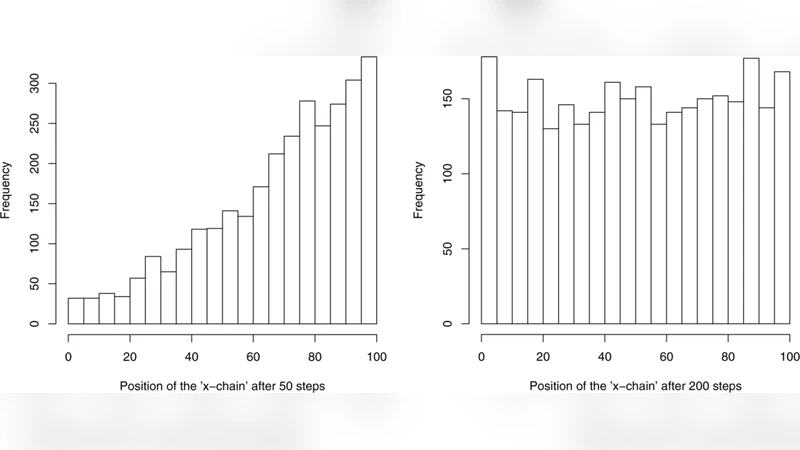
For each case the paper computes the exact eigenfunctions, eigenvalues, and demonstrates numerically that the empirical convergence of the Gibbs sampler matches the theoretical (\rho^{t}) decay. Moreover, the orthogonal‑polynomial expansion provides closed‑form expressions for autocorrelation functions of any observable, allowing precise calculation of effective sample sizes and other diagnostic quantities.

Beyond the theoretical analysis, the paper discusses practical implications. Since (\rho) is directly controllable through prior hyper‑parameters, one can deliberately choose priors that enlarge the spectral gap and thus accelerate convergence. The diagonalization also suggests optimal block‑updating schemes: by grouping variables whose conditional updates correspond to low‑degree polynomial components, one can reduce the effective (\rho) and improve mixing. These insights bridge the gap between abstract spectral theory and concrete MCMC algorithm design, especially for high‑dimensional Bayesian hierarchical models where standard convergence diagnostics are often unreliable.

In summary, the work provides a unified framework that links exponential‑family structure, conjugate priors, and classical orthogonal polynomials to obtain exact spectral decompositions of Gibbs samplers. This yields precise, non‑asymptotic convergence rates, explicit formulas for autocorrelations, and actionable guidance for improving sampler efficiency. The results deepen our understanding of why Gibbs sampling works so well in many conjugate settings and open avenues for extending the approach to more complex, possibly non‑conjugate, models through approximate polynomial bases or spectral perturbation techniques.