On Field Size and Success Probability in Network Coding

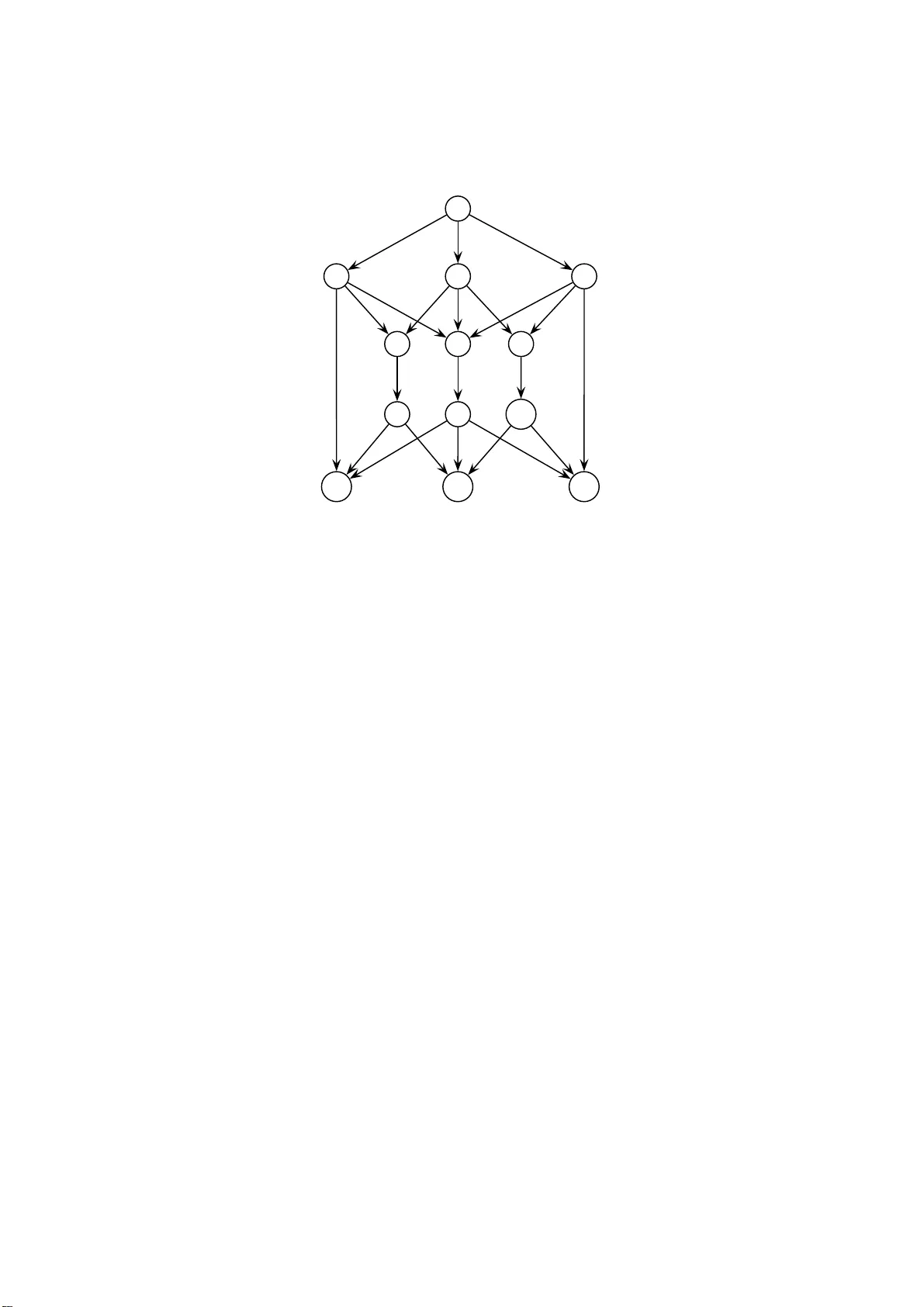
On Field Size a nd Success Probabilit y in Net w ork Co ding Ola v Geil ∗ , Ryutaroh Matsumoto † , Casp er Thomsen ‡ Octob er 31, 201 8 Abstract Using tools from algebraic geometry and Gr¨ obner basis theory we sol ve tw o problems in netw ork coding. First we present a metho d to determine the smallest field size for which linear netw ork co ding is feasible. Second w e deriv e impro ved estimates on the success probabilit y of random lin- ear netw ork co ding. These estimates take into account whic h monomials occur in the supp ort of the determinant of t he prod uct of Edmonds ma- trices. Therefore we fin ally inv estigate which monomial s can o ccur in the determinant of the Edmonds matrix. Keywords. Distribu ted net w orking, linear netw ork coding, multicast, netw ork co ding, random netw ork co ding. 1 In tro duction In a traditional data netw or k, a n in termediate no de only forwards data and never mo difies them. Ahlswede et al. [1] show ed that if we a llow in termedi- ate no des to pr o cess their incoming data and output mo dified versions of them then maximum throughput can increase, and they also s howed that the maxi- m um thro ughput is given by the minimum of maxflows b etw een the so urce no de and a sink no de for single sour ce multicast on an a cyclic directional netw ork. Such pr o cessing is called net work co ding. Li et al. [10] showed that computa- tion of linear com binations ov er a finite field by intermediate no des is eno ugh for achieving the maximu m throughput. Net work co ding only inv olving linear combinations is ca lled linear netw ork co ding. The a cyclic assumption was later remov ed by Ko etter a nd M´ edard [9]. In this pap er we shall concentrate on the er ror-fr ee, delay-free multisource m ulticast netw ork connectio n problem wher e the s ources are unco r related. How- ever, the prop o s ed metho ds descr ibe d can be g eneralized to de a l with delays as in [7]. The only exception is the descr iptio n in Section 7. Considering multicast, it is imp ortant to decide whether or not all re c eivers (called sinks) can recover all the transmitted information from the senders ∗ Departmen t of Mathematical Sciences, Aalborg Univ ersity , Denmark, olav@math.aau. dk † Departmen t of Communicat ions and Int egrated Systems, T okyo Institute of T echnology , Japan ryuta roh@rmat sumoto.or g ‡ Departmen t of Mathematical Sciences, Aalb org Unive rsity , Denmark, caspert@ math.aau. dk 1 (called sources ). It is also imp ortant to decide the minim um size q of the finite field F q required for linea r netw o rk co ding. Before using linea r netw o rk co ding we hav e to decide co efficients in linear combinations computed b y intermediate nodes. When the size q of a finite field is large, it is shown that random choice of coefficients allo ws all sinks to recover the origina l tr a nsmitted information with high probability [7]. Suc h a metho d is ca lled ra ndom linear net work co ding and the probability is ca lled success probability . As to random linear net w ork coding the estimation or determination of the success pr obability is very imp ortant. Ho et a l. [7 ] gav e a low er bo und on the success pr obability . In their pap er [9], Ko etter and M ´ edard introduced an algebr aic geometric po int view on netw o rk co ding. As expla ined in [3], c omputational problems in algebra ic geo metry ca n often b e solved by Gr ¨ obner ba ses. In this pap er, we shall show that the exa ct computation of the minim um q can b e made by applying the divisio n algorithm for multiv ariate p olynomia ls, and we will show that improv ed estima tes for the success proba bility can be found by applying the fo otpr in t b ound from Gr¨ obner basis theory . These r esults introduce a new approach to net w ork c o ding study . As the improved estimates take into account which monomials o ccur in the s uppo r t of the deter minant o f a certain ma tr ix [7] we study this matrix in details a t the end of the pap er. 2 Preliminary W e can deter mine whether or not all sinks can recover all the transmitted infor - mation by the determinant of some matrix [7]. W e sha ll r e v iew the definition of such determinant. Let G = ( V , E ) b e an directed acyclic g raph with p ossible parallel edges that repr e sents the netw ork top olog y . The s e t o f so urce a nd s ink no des is denoted b y S and T resp ectively . Assume that the source no des S together get h symbols in F q per unit time and try to send them. Ident ify the edges in E with the integers 1 , . . . , | E | . F or an edge j = ( u, v ) we write hea d( j ) = v and tail( j ) = u . W e define the | E | × | E | matrix F = ( f i,j ) where f i,j is a v ariable if head( i ) = tail( j ) and f i,j = 0 otherwise. The v aria ble f i,j is the co ding co efficient from i to j . Index h symbols in F q sent by S by 1 , . . . , h . W e a lso define an h × | E | matrix A = ( a i,j ) wher e a i,j is a v ar iable if the edge j is an outgoing edge fr om the source s ∈ S sending the i -th symbol and a i,j = 0 otherwise. V ariables a i,j represent how the so urce no des send information to their o utgoing edges. Let X ( l ) denote the l -th s y m bo l generated by the sour ces S , and let Y ( j ) de- note the information sent along edg e j . The mo del is described b y the follo wing relation Y ( j ) = h X i =1 a i,j X ( i ) + X i :head( i )=tail( j ) f i,j Y ( i ) . F or each sink t ∈ T define an h × | E | matrix B t whose ( i, j ) entry b t,i,j is a v aria ble if head( j ) = t and equals 0 otherwise. The index i refers to the i -th symbol sent by one o f the s o urces. Thereby v ariables b t,i,j represent how the sink t pro ces s the received data fro m its incoming edges . The sink t reco rds the vector ~ b ( t ) =  b ( t ) 1 , . . . , b ( t ) h  2 where b ( t ) i = X j :head( j )= t b t,i,j Y ( j ) . W e now recall from [7 ] under which conditions all informations sent by the sources can alwa y s b e recov ered at all sinks. As in [7] we define the Edmonds matrix M t for t ∈ T by M t =  A 0 I − F B T t  . (1) Define the p olynomia l P by P = Y t ∈ T | M t | . (2) P is a multiv a riate polyno mia l in v a r iables f i,j , a i,j and b t,i,j . Assigning a v alue in F q to each v aria ble co rresp onds to choo sing a co ding scheme. Plugg ing the assigned v alues into P gives an elemen t k ∈ F q . The following theorem from [7] tells us w he n the co ding scheme can b e used to alwa ys r ecov er the information generated at the sources S at all sinks in T . Theorem 1. L et t he n otation and the net work c o ding mo del b e as ab ove. As- sume a c o ding scheme has b e en chosen by assigning values to the variables f i,j , a i,j and b t,i,j . L et k b e t he value found by plugging the assigne d values into P . Every sink t ∈ T c an r e c over fr om ~ b ( t ) the informations X (1) , . . . , X ( h ) no matter what they ar e, if and only if k 6 = 0 holds. Pr o of. See [7]. 3 Computation of the Minim um Field S ize W e shall study computation of the minim um sym bo l size q . F or this purpose we will need the division algorithm for multiv a riate p oly nomials [3, Sec. 2.3 ] to pro- duce the remainder of a p olynomial F ( X 1 , . . . , X n ) mo dulo ( X q 1 − X 1 , . . . , X q n − X n ) (this remainder is indep endent of the choice of monomial or dering). W e adapt the standar d notation for the a bove remainder which is F ( X 1 , . . . , X n ) rem ( X q 1 − X 1 , . . . , X q n − X n ) . The reader unfamiliar with the divisio n algorithm can think o f the ab ov e remain- der of F ( X 1 , . . . , X n ) as the p olynomia l pro duce d by the following pr o cedure. As long as we can find an X i such that X q i divides some term in the p olyno mial under consideratio n we replac e the factor X q i with X i wherever it occur s. The pro cess c ontin ues until the X i -degree is less than q for a ll i = 1 , . . . , n . It is clear that the ab ove pro cedure can b e efficiently implemented. Prop ositio n 2. L et F ( X 1 , . . . , X n ) b e an n - variate p olynomial over F q . Ther e exists an n -tu ple ( x 1 , . . . , x n ) ∈ F n q such that F ( x 1 , . . . , x n ) 6 = 0 if and only if F ( X 1 , . . . , X n ) rem ( X q 1 − X 1 , . . . , X q n − X n ) 6 = 0 . Pr o of. As a q = a for all a ∈ F q it holds that F ( X 1 , . . . , X n ) ev alua tes to the same as R ( X 1 , . . . , X n ) := F ( X 1 , . . . , X n ) rem ( X q 1 − X 1 , . . . , X q n − X n ) in every ( x 1 , . . . , x n ) ∈ F n q . If R ( X 1 , . . . , X n ) = 0 ther e fore F ( X 1 , . . . , X n ) ev aluates 3 to zero for every choice of ( x 1 , . . . , x n ) ∈ F n q . If R ( X 1 , . . . , X n ) is nonzero we consider it first a s a p olyno mial in F q ( X 1 , . . . , X n − 1 )[ X n ] (that is, a p olyno mial in one v ariable ov er the quotient field F q ( X 1 , . . . , X n − 1 )). But the X n -degree is at most q − 1 a nd there fore it ha s a t mos t q − 1 zer os. W e conclude tha t there exists an x n ∈ F q such that R ( X 1 , . . . , X n − 1 , x n ) ∈ F q [ X 1 , . . . , X n − 1 ] is nonzero. Contin uing this wa y we find ( x 1 , . . . , x n ) such that R ( x 1 , . . . , x n ) a nd therefore also F ( x 1 , . . . , x n ) is no nz e r o. F rom [7, Th. 2] we know that fo r all prime p ow e r s q g reater than | T | linear net work co ding is p ossible. It is now straig ht forward to describ e an algor ithm that finds the smallest field F q of pr escrib ed characteristic p for which linear net work co ding is feasible. W e first r educe the p olynomia l P from (2) mo dulo the prime p . W e obser ve that a lthough P is a p olynomial in all the v a riables a i,j , b t,i,j , f i,j the v aria ble b t,i,j app ears at most in p ow ers o f 1 . This is so as it a ppea rs at most in a single entry in M t and do es no t app ear elsewher e. Therefore F q can be use d for net work coding if P rem p does not reduce to zero mo dulo the p olynomials a q i,j − a i,j , f q i,j − f i,j . T o decide the smallest field F q of characteristic p for which netw ork co ding is feasible we try first F q = F p . If this do es not work w e then try F p 2 and so on. T o find an F q that works we need at most to try ⌊ log p ( | T | ) ⌋ different fields as we know that linea r net w ork co ding is p oss ible w he never q > | T | . Note tha t once a field F q is found such that the netw ork connectio n pr oblem is feasible the last part o f the pr o of of P rop osition 1 describ es a simple way o f deciding co efficients ( x 1 , . . . , x n ) ∈ F n q that can be used for netw ork co ding . F rom [4 , Sec. 7 .1.3] we know that it is a n NP-ha rd problem to find the minim um field size for linear netw ork co ding. Our findings imply that it is NP-hard to find the p olynomial P in (2). 4 Computation of the Suc cess Probabilit y of Ran- dom Linear Net w ork Co ding In rando m linear netw ork co ding we fro m the b eginning fix for a collec tio n K ⊆ { 1 , . . . , h } × { 1 , . . . , | E |} the a i,j ’s with ( i, j ) ∈ K and also we fix for a collection J ⊆ { 1 , . . . , | E |} × { 1 , . . . , | E |} the f i,j ’s with ( i, j ) ∈ J . This is done in a wa y suc h that there exis ts a solution to the netw ork connec tio n problem with the same v alues for these fixed co efficients. A prio ri of cour se we let a i,j = 0 if the edge j is no t emer ging from the sour ce sending informa tion i , and als o a pr iori we of cour s e let f i,j = 0 if j is not an adjacent do wnstream edge o f i . Bes ide s these a prio ri fixed v alues there may be g o o d rea sons for also fixing o ther co efficients a i,j and f i,j [7]. If for example there is only one upstream edge i adjacent to j we may assume f i,j = 1. All the a i,j ’s and f i,j ’s which hav e not b een fixed at this p oint are then c hosen randomly and indep endently . All co efficients a re to b e element s in F q . If a solution to the netw ork connection proble m exists with the a i,j ’s and the f i,j ’s sp ecified, it is p ossible to determine v alues of b t,i,j at the sinks s uch that a solution to 4 the netw o r k co nnec tion pr oblem is given. Le t µ be the n umber of v ar iables a i,j and f i,j chosen randomly . Call these v ariables X 1 , . . . , X µ . Co nsider the po lynomial P in (2) and let e P b e the p olynomial made from P by plugging in the fixed v a lues of the a i,j ’s and the fixed v a lues of the f i,j ’s (calculations ta k ing place in F q ). Then e P is a p olynomial in X 1 , . . . , X µ . The co efficients of e P are po lynomials in the b t,i,j ’s ov er F q . Fina lly , define b P := e P rem ( X q 1 − X 1 , . . . , X q µ − X µ ) . The success probability of random linear netw ork c o ding is the proba bility that the rando m c hoice of co efficients will lead to a s olution of the netw o rk connection problem 1 as in Section 2. Tha t is, the pro bability is the num ber |{ ( x 1 , . . . , x µ ) ∈ F µ q | e P ( x 1 , . . . , x µ ) 6 = 0 }| q µ = |{ ( x 1 , . . . , x µ ) ∈ F µ q | b P ( x 1 , . . . , x µ ) 6 = 0 }| q µ . (3) T o see the first result observe that for fixed ( x 1 , . . . , x µ ) ∈ F µ q , e P ( x 1 , . . . , x µ ) can be view ed as a p olyno mial in the v ariables b t,i,j ’s with co efficients in F q and recall that the b t,i,j ’s o ccur in p ow ers o f at most 1 . Ther efore, if e P ( x 1 , . . . , x µ ) 6 = 0, then by Prop ositio n 2 it is p ossible to choo se the b t,i,j ’s such that if we plug them into e P ( x 1 , . . . , x µ ) then we g e t nonzero. The last res ult follows from the fact that e P ( x 1 , . . . , x µ ) = b P ( x 1 , . . . , x µ ) for all ( x 1 , . . . , x µ ) ∈ F µ q . In this section we shall pre s ent a metho d to e s timate the success pro ba bilit y us ing Gr¨ obner basis theoretica l metho ds. W e br iefly review some ba sic definitions and r esults o f Gr¨ obner bases. See [3] for a mor e detailed exp osition. Let M ( X 1 , . . . , X n ) b e the set of monomials in the v ar ia bles X 1 , . . . , X n . A mo nomial orde r ing ≺ is a total or de r ing on M ( X 1 , . . . , X n ) such tha t L ≺ M = ⇒ LN ≺ M N holds for all monomials L , M , N ∈ M ( X 1 , . . . , X n ) and suc h that every nonempt y subset of M ( X 1 , . . . , X n ) has a unique smallest elemen t with respect to ≺ . The leading monomial of a p oly nomial F with re spe ct to ≺ , denoted by lm ( F ), is the lar gest monomial in the supp or t of F . Given a po lynomial idea l I and a monomial order ing the fo otprint ∆ ≺ ( I ) is the set of monomials that c a nnot be found a s leading mo no mials of any p olynomial in I . The following prop osi- tion explains our interest in the fo otprint (for a pro o f o f the prop osition se e [2, Pro. 8.32]). Prop ositio n 3. L et F b e a field and c onsider the p olynomi als F 1 , . . . , F s ∈ F [ X 1 , . . . , X n ] . L et I = h F 1 , . . . , F s i ⊆ F [ X 1 , . . . , X n ] b e the ide al gener ate d by F 1 , . . . , F s . If ∆ ≺ ( I ) is fi nite then the numb er of c ommon zer os of F 1 , . . . , F s in the algebr aic closur e of F is at m ost e qual to | ∆ ≺ ( I ) | . Prop ositio n 3 is known a s the fo otprint b ound. It has the following corolla ry . 1 This c orresp onds to saying that each sink can reco ver the d ata at the maximu m rate promised b y net wo rk codi ng. 5 Corollary 4. Le t F ∈ F [ X 1 , . . . , X n ] wher e F is a field c ontaining F q . Fix a monomial or dering and let X j 1 1 · · · X j n n = lm  F rem ( X q 1 − X 1 , . . . , X q n − X n )  . The numb er of zer os of F over F q is at most e qual to q n − n Y v =1 ( q − j v ) . (4) Pr o of. W e hav e ∆ ≺ ( h F, X q 1 − X 1 , . . . , X q n − X n i ) ⊆ ∆ ≺ ( h lm ( F r em ( X q 1 − X 1 , . . . , X q n − X n )) , X q 1 , . . . , X q n i ) and the siz e of the latter s et equa ls (4). The result now follows immediately from Prop os ition 3. Theorem 5. L et as ab ove e P b e found by plugging into P some fix e d values for the variables a i,j , ( i, j ) ∈ K , and by plugging into P some fixe d values for the variables f i,j , ( i, j ) ∈ J , and by le aving the r emaining µ variables flexible. Assume as ab ove t hat ther e exists a solution to the network c onn e ction pr oblem with the same values for these fixe d c o efficients. Denote by X 1 , . . . , X µ the variables to b e chosen by r andom and define b P := e P rem ( X q 1 − X 1 , . . . , X q µ − X µ ) . (Note that if q > | T | then b P = e P ). Consider b P as a p olynomial in t he variables X 1 , . . . , X µ and let ≺ b e any fixe d monomial or dering. Writing X j 1 1 · · · X j µ µ = lm ( b P ) t he suc c ess pr ob ability is at le ast q − µ µ Y v =1 ( q − j v ) . (5) As a c onse quenc e the suc c ess pr ob ability is in p articular at le ast q − µ min  µ Y i =1 ( q − s i )     X s 1 1 · · · X s µ µ is a monomial in the su pp ort of b P  . (6) Pr o of. Let F b e the quotient field F q ( X 1 , . . . , X µ ). The result in (5) now follows by applying Corollar y 4 and (3). As the lea ding monomial of e P is of co ur se a monomial in the suppo rt of e P (6) is s maller or eq ua l to (5). Remark 6. The c ondition in The or em 5 that ther e exists a solution t o t he network c onne ction pr oblem with t he c o efficients c orr esp onding t o K and J b eing as sp e cifie d is e quivalent to the c ondition that b P 6 = 0 . W e conclude this s ection by mentioning without a pro of that Gr¨ obner basis theory tells us tha t the true succes s probability ca n b e calculated as q − µ  q µ − | ∆ ≺ ( h e P , X q 1 − X 1 , . . . , X q µ − X µ i ) |  . This obser v ation is how ev er of little v alue as it seems very difficult to compute the fo otprint ∆ ≺ ( h e P , X q 1 − X 1 , . . . , X q µ − X µ i ) due to the fact that µ is typically a very high nu mber. 6 5 The B ound by Ho et al. In [7] Ho et a l. gave a lower b ound on the success probability in terms of the nu mber of edges j with asso ciated random co efficients 2 { a i,j , f l,j } . Letting η b e the num b er of such edges [7, Th. 2] tells us that if q > | T | and if there exists a solution to the netw o rk co nnection problem with the same v alues for the fixed co efficients, then the s uccess probability is at least p Ho =  q − | T | q  η . (7) The pro of in [7 ] of (7) relies on t w o lemmas of which w e o nly state the first one. Lemma 7 . L et η b e define d as ab ove. The determinant p olynomia l of M t has maximum de gr e e η in the r andom variables { a i,j , f l,j } and is line ar in e ach of these variables. Pr o of. See [7, Lem. 3 ]. Alternatively the pro o f can b e derived as a consequence of Theor e m 11 in Section 7. Recall, that the p olynomia l P in (2) is the pro duct of the determinants | M t | , t ∈ T . Lemma 7 ther e fore implies tha t the p olynomia l e P has at most total degree equal to | T | η and that no v a riable app ears in powers of more than | T | . The ass umption q > | T | implies b P = e P which makes it par ticular easy to see that the s ame o f cour se holds for b P . Combining this observ a tion with the following lemma sho ws tha t the num ber s in (5 ) and (6) are b o th at least as large as the num ber (7). Lemma 8. L et η , | T | , q ∈ N , | T | < q b e some fixe d nu mb ers. L et µ, x 1 , . . . , x µ ∈ N 0 satisfy 0 ≤ x 1 ≤ | T | , . . . , 0 ≤ x µ ≤ | T | and x 1 + · · · + x µ ≤ | T | η . The minimal value of µ Y i =1  q − x i q  (taken over al l p ossible values of µ, x 1 , . . . , x µ ) is  q − | T | q  η . Pr o of. Assume µ and x 1 , . . . , x µ are chosen such that the expressio n attains its minimal v a lue . Without lo ss of genera lity we may assume that x 1 ≥ x 2 ≥ · · · ≥ x µ holds. Clearly , x 1 + · · · + x µ = | T | η must hold. If x i < | T | a nd x i +1 > 0 then ( q − x i )( q − x i +1 ) > ( q − ( x i + 1))( q − ( x i +1 − 1)) which ca nnot b e the case. So x 1 = · · · = x η = | T | . The remaining x j ’s if any all equal zero . 2 W e state Ho et al.’s bound only in the case of delay -free acyc lic net works. 7 v 1 v 2 v 3 v 4 v 5 v 6 v 7 v 8 v 9 v 10 v 11 v 12 v 13 1 2 3 4 5 6 7 8 9 10 11 12 13 14 15 16 17 18 Figure 1: The netw o rk fr om Example 9 6 Examples In this section w e apply the metho ds from the previous sections to tw o concrete net works. W e will see that the estimate on the success probability of random linear netw o rk co ding that was descr ib e d in Theorem 5 can b e c o nsiderably better than the estimate describ ed in [7, Th. 2]. Also we w ill apply the metho d from Section 3 to determine the smalles t field of character istic t wo for which net work co ding can b e successful. As random linear netw o rk co ding is a ssumed to ta ke pla ce at the no des in a decentralized manner, o ne natural choice is to set f i,j = 1 whenever the indegree of the end no de of edge i is one and j is the downstream edge adjacent to i . Clearly , if j is no t a downstream edge adjacent to i we set f i,j = 0. Whenev er none of the ab ov e is the case we may c ho ose f i,j randomly . Also if there is only one source and the outdeg r ee of the so urce is eq ual to the num ber of symbols to be send we may enumerate the edges from the s ource by the num be r s 1 , . . . , h and s et a i,j = 1 if 1 ≤ i = j ≤ h and s et a i,j = 0 other wise. T his strategy can be generalized also to de a l with the case o f more so urces. In the following t wo exa mples we will choo se the v ariables in the manner just des crib ed. The net work in the first example is taken from [4, Ex. 3 .1] whereas the net work in the second exa mple is new. Example 9. Consider the delay-fr e e and acyclic n etwork in Figur e 1. Ther e is one sender v 1 and two r e c eivers v 12 and v 13 . The min-cut max-flow num b er is two for b oth r e c eivers so we assum e that two indep endent ra ndom pr o c esses emer ge fr om sender v 1 . We c onsider in this example only fi elds of char acteristic 8 T able 1: F rom Example 9: Estimates on the succe ss probability q 4 8 16 32 64 P new 1 ( q ) 0.140 0.430 0 .672 0.8 93 0.909 P new 2 ( q ) 0 . 703 × 10 − 1 0.322 0 .588 0.7 73 0.880 P Ho ( q ) 0 . 625 × 10 − 1 0.316 0 .586 0.7 72 0.880 2 . F ol lowing the description pr e c e ding the example we set a 1 , 1 = a 2 , 2 = 1 and a i,j = 0 in al l other c ases. Also we let f i,j = 1 exc ept f 3 , 7 , f 5 , 7 , f 4 , 10 , f 8 , 10 , f 9 , 11 , f 6 , 11 , f 12 , 16 , f 14 , 16 which we cho ose by r andom. As in the pr evio us se ctions we c ons ider b t,i,j as fixe d but unknown to us . The determinant p olynomi al b e c omes e P = ( b 2 c 2 e 2 g h + c 2 f 2 g h + a 2 d 2 f 2 g h ) Q, wher e a = f 3 , 7 b = f 5 , 7 c = f 4 , 10 d = f 8 , 10 e = f 9 , 11 f = f 6 , 11 g = f 12 , 16 h = f 14 , 16 and Q = | B ′ v 12 | | B ′ v 13 | . Her e, B ′ v 12 r esp e ctively B ′ v 13 is the matrix c onsisting of t he nonzer o c olumn s of B v 12 r esp e ctively the nonzer o c olumns of B v 14 . Re- stricting to fields F q of size at le ast 4 we have b P = e P and we c an ther efor e imme diately apply the b ounds in The or em 5. Applying (6) we get the fol lowing lower b oun d on t he suc c ess pr ob ability P new 2 ( q ) = ( q − 2) 3 ( q − 1) 2 q 5 . Cho osing as monomial or dering t he lexic o gr aphic or dering ≺ lex with a ≺ lex b ≺ lex d ≺ lex e ≺ lex g ≺ lex h ≺ lex f ≺ lex c the le ading monomial of e P b e c omes c 2 f 2 g h and ther efor e fr om (5 ) we get the fol lowing lower b ound on the su c c ess pr ob ability P new 1 ( q ) = ( q − 2) 2 ( q − 1) 2 q 4 . F or c omp arison the b ound (7) fr om [7] states that the su c c ess pr ob ability is at le ast P Ho ( q ) = ( q − 2) 4 q 4 . We se e that P new 1 exc e e ds P Ho with a factor ( q − 1) 2 / ( q − 2) 2 , which is lar ger than 1. Also P new 2 exc e e ds P Ho . In T able 1 we list values of P new 1 ( q ) , P new 2 ( q ) and P Ho ( q ) for various choi c es of q . We next c onsider the field F 2 . W e r e duc e e P mo dulo ( a 2 − a, . . . , h 2 − h ) to get b P = ( b ceg h + cf g h + ad f g h ) Q. 9 v 1 v 2 v 3 v 4 v 5 v 6 v 7 v 8 v 9 v 10 v 11 v 12 v 13 1 2 3 4 5 6 7 8 9 10 11 12 13 14 15 16 17 18 19 20 21 22 Figure 2: The netw o rk fr om Exa mple 10 F r om (6) we se e that the suc c ess pr ob ability of r andom network c o ding is at le ast 2 − 5 . Cho osing as monomial or dering the lexic o gr aphic or dering describ e d ab ove (5) tel ls u s that the suc c ess pr ob ability is at le ast 2 − 4 . F or c omp arison the b oun d (7) do es not apply as we do not have q > | T | . It should b e m entione d that for delay-fr e e acyclic networks the network c o ding pr oblem is solvable for al l choic es of q ≥ | T | [8] and [11]. F r om this fact one c an only c onclude that the suc c ess pr ob abili ty is at le ast 2 − 8 (8 b eing the numb er of c o efficients to b e chosen by r andom). Example 10. Consider the network in Figur e 2 . The sender v 1 gener ates 3 indep endent r andom pr o c esses. The vertic es v 11 , v 12 and v 13 ar e the r e c eivers. We wil l apply network c o ding over various fields of char acteristic two. We start by c onsidering r andom line ar net work c o ding over fields of size at le ast 4 . As 4 > | T | = 3 we kn ow that this c an b e done suc c essful ly. We set a 1 , 1 = a 2 , 2 = a 3 , 3 = 1 and a i,j = 0 in al l other c ases. We let f i,j = 1 exc ept f 4 , 13 , f 7 , 13 , f 5 , 14 , f 8 , 14 , f 10 , 14 , f 9 , 15 , f 11 , 15 , which we cho ose by r andom. As in t he last se ction we c onsider b t,i,j as fix e d but unknown to us. Ther efor e e P = b P is a p olynomial in the seven variable s f 4 , 13 , f 7 , 13 , f 5 , 14 , f 8 , 14 , f 10 , 14 , f 9 , 15 , f 11 , 15 . The determinant p olynomia l b e c omes b P = ( ab cdef g + abc e 2 f 2 + b 2 c 2 ef g ) Q, wher e a = f 4 , 13 b = f 5 , 14 c = f 7 , 13 d = f 8 , 14 e = f 9 , 15 f = f 10 , 14 g = f 11 , 15 and Q = | B ′ v 11 | | B ′ v 12 | | B ′ v 13 | . H er e, B ′ v 11 r esp e ctively B ′ v 12 r esp e ctively B ′ v 13 is the matrix c onsisting of the nonzer o c olumn s of B v 11 r esp e ctively t he nonzer o c olumns of B v 12 r esp e ctively t he n onz er o c olumns of B v 13 . Cho osing a lexic o- gr aphic or dering with d b eing lar ger than the other variables and applying (5) 10 T able 2: F ro m E xample 10: Estimates on the s uccess probability q 4 8 16 32 64 P new 1 ( q ) 0.133 0.392 0 .636 0.8 00 0.895 P new 2 ( q ) 0.105 0.376 0 .630 0.7 99 0.895 P Ho ( q ) 0 . 156 × 10 − 1 0.244 0 .536 0.7 44 0.865 we get that the suc c ess pr ob ability is at le ast P new 1 ( q ) = ( q − 1) 7 q 7 . Applying (6) we se e that the su c c ess pr ob ability is at le ast P new 2 ( q ) = ( q − 1) 3 ( q − 2) 2 q 5 . F or c omp arison (7 ) tel ls us that suc c ess pr ob ability is at le ast P Ho ( q ) = ( q − 3) 3 q 3 . Both b ound (5) and b ound (6) ex c e e d (7) for al l values of q ≥ 4 . In T able 2 we list P new 1 ( q ) , P new 2 ( q ) and P Ho ( q ) for various values of q . We nex t c onsider the field F 2 . We r e duc e e P mo dulo ( a 2 − a, . . . , g 2 − g ) t o get b P = ( abcdef g + abcef + bce f g ) Q. F r om (6) we se e that the suc c ess pr ob abili ty of r andom network c o ding is at le ast 2 − 7 . Cho osing a pr op er monomial or dering we get fr om (5) that the su c c ess pr ob ability is at le ast 2 − 5 . F or c omp arison n either [7], [8], nor [11] tel ls us that line ar network c o ding is p ossible. 7 The T op ological Meaning of | M t | Recall fr om Section 5 that Ho et al.’s b o und (7 ) relies on the ra ther roug h Lemma 7 . The following theo rem g ives a muc h mo re precise descr iption o f which mono mials can o ccur in the suppo rt of P a nd e P by explaining exactly which mono mials can o ccur in | M t | . Thereby the theorem gives so me insight int o when the b o unds (5) and (6) are m uch b etter than the bound (7). The theorem states that if K is a monomial in the suppo rt of | M t | then it is the pro duct of a i,j ’s, f i,j ’s a nd b t,i,j ’s related to h edge disjoint paths P 1 , . . . , P h that orig inate in the senders a nd end in receiver t . Theorem 11. Consider a delay-fr e e acyclic network. If K is a m onomial in the supp ort of the determinant of M t then it is of the form K 1 · · · K h wher e K u = a u,l ( u ) 1 f l ( u ) 1 ,l ( u ) 2 f l ( u ) 2 ,l ( u ) 3 · · · f l ( u ) s u − 1 ,l ( u ) s u b t,v u ,l ( u ) s u for u = 1 , . . . , h . Her e, { v 1 , . . . , v h } = { 1 , . . . , h } holds and l (1) 1 , . . . , l ( h ) h r esp e c- tively l (1) s 1 , . . . , l ( h ) s h ar e p airwise differ ent. F urther f l ( u 1 ) i ,l ( u 1 ) i +1 6 = f l ( u 2 ) j ,l ( u 2 ) j +1 11 s v 1 v 2 v 3 v 4 t 1 t 2 1 4 2 5 3 6 7 8 9 Figure 3: The butterfly netw ork unless u 1 = u 2 and i = j hold. In other wor ds K c orr esp onds to a pr o duct of h e dge disjoint p aths. Pr o of. A pr o of can b e found in the app endix. W e illustra te the theorem with a n ex ample. Example 12. Consider the butterfly n et work in Figur e 3. A monomial K is in the supp ort of | M t 1 | if and only if it is in the supp ort of the determinant of N t 1 = ( n i,j ) =  I + F B T t 1 A 0  =                   1 0 f 1 , 3 f 1 , 4 0 0 0 0 0 0 0 0 1 0 0 f 2 , 5 f 2 , 6 0 0 0 0 0 0 0 1 0 0 0 0 0 0 b t 1 , 1 , 3 b t 1 , 2 , 3 0 0 0 1 0 0 f 4 , 7 0 0 0 0 0 0 0 0 1 0 f 5 , 7 0 0 0 0 0 0 0 0 0 1 0 0 0 0 0 0 0 0 0 0 0 1 f 7 , 8 f 7 , 9 0 0 0 0 0 0 0 0 0 1 0 b t 1 , 1 , 8 b t 1 , 2 , 8 0 0 0 0 0 0 0 0 1 0 0 a 1 , 1 a 1 , 2 0 0 0 0 0 0 0 0 0 a 2 , 1 a 2 , 2 0 0 0 0 0 0 0 0 0                   By insp e ction we se e that the monomial K = a 1 , 1 a 2 , 2 b t 1 , 1 , 3 b t 1 , 2 , 8 f 7 , 8 f 5 , 7 f 2 , 5 f 1 , 3 is in the supp ort of | N t 1 | . We c an write K = K 1 K 2 wher e K 1 = a 1 , 1 f 1 , 3 b t 1 , 1 , 3 and K 2 = a 2 , 2 f 2 , 5 f 5 , 7 f 7 , 8 b t 1 , 2 , 8 . This is the description guar ante e d by The or em 11. T o make it e asier for the r e ader to fol low t he pr o of of The or em 11 in the app endix we now intr o duc e some of the notations to b e use d ther e. By insp e ction the monomial K c an b e written K = 11 Y i =1 n i,p ( i ) 12 wher e the p ermutation p is given by p (1) = 3 p (2) = 5 p (3) = 10 p (4 ) = 4 p (5) = 7 p (6) = 6 p (7) = 8 p (8) = 11 p (9) = 9 p (10 ) = 1 p (11) = 2 Ther efor e if we index the elements in { 1 , . . . , 11 } by i 1 = 10 i 2 = 1 i 3 = 3 i 4 = 11 i 5 = 2 i 6 = 5 i 7 = 7 i 8 = 8 i 9 = 4 i 10 = 6 i 11 = 9 then we c an write K 1 = n i 1 ,p ( i 1 ) n i 2 ,p ( i 2 ) n i 3 ,p ( i 3 ) K 2 = n i 4 ,p ( i 4 ) n i 5 ,p ( i 5 ) n i 6 ,p ( i 6 ) n i 7 ,p ( i 7 ) n i 8 ,p ( i 8 ) and we have n i 9 ,p ( i 9 ) = n i 10 ,p ( i 10 ) = n i 11 ,p ( i 11 ) = 1 c orr esp onding to the fact p ( i 9 ) = i 9 , p ( i 10 ) = i 10 and p ( i 11 ) = i 11 . Remark 13. The pr o c e dur es describ e d in the pr o of of The or em 11 c an b e re - verse d. This implies that ther e is a bije ctive map b etwe en the set of e dge disjoi nt p aths P 1 , . . . , P h in The or em 11 and the set of monomials in | M t | . Theorem 11 immediately applies to the situation of r andom netw ork co ding if we plug into the a i,j ’s a nd into the f t,i,j ’s o n the pa ths P 1 , . . . , P h the fixed v alues wherever such ar e given. Let as in Lemma 7 η be the n um be r o f edges for which s o me co efficients a i,j , f i,j are to b e chosen b y random. Co nsidering the deter minant as a p olynomial in the v ariables to b e chosen b y ra ndom with co efficients in the field o f r ational expres sions in the b t,i,j ’s we see that no mono- mial can contain mo r e than η v aria bles and that no v ar iable o ccur s more than once. This is b ecause the paths P 1 , . . . , P h are edge disjoint. Hence, Lemma 7 is a cons equence o f Theorem 11. 8 Ac kno wledgmen ts The a utho rs would like to thank the anonymous refere e s fo r their he lpful sug- gestions. A Pro of of Theorem 11 The pro of of Theo r em 11 calls for the following technical lemma. Lemma 14. Consider a delay-fr e e acyclic n et work with c orr esp onding matrix F as in Se ction 2. L et I b e the | E | × | E | identity matrix and define Γ = ( γ i,j ) = I + F. Given a p erm u tation p on { 1 , . . . , | E |} write p ( i ) ( λ ) = i times z }| { p ( p ( · · · ( λ ) · · · )) If for some λ ∈ { 1 , . . . , | E |} t he fol lowing hold 13 (1) λ, p ( λ ) , . . . , p ( x ) ( λ ) ar e p airwise differ ent (2) p ( x +1) ( λ ) ∈ { λ, p ( λ ) , . . . , p ( x ) ( λ ) } (3) γ λ,p ( λ ) , γ p ( λ ) ,p ( p ( λ )) , . . . , γ p ( x ) ( λ ) ,p ( x +1) ( λ ) ar e al l nonzer o then x = 0 . Pr o of. Let p be a permutation a nd let x and λ b e n um ber s such that (1), (2) and (3) hold. As p is a p ermutation then (1) and (2) implies that p ( p ( x ) ( λ )) = λ . Aiming for a contradiction assume x > 0. As p ( η ) = η do es not hold for any η ∈ { λ, p ( λ ) , . . . , p ( x ) ( λ ) } , γ λ,p ( λ ) , γ p ( λ ) ,p (2) ( λ ) , . . . , γ p ( x ) ( λ ) ,p ( x +1) ( λ ) are all non-diago nal elements in I + F . By (3) we therefore hav e constructed a cycle in a cycle -free graph and the assumption x > 0 canno t b e true. of The or em 11 . A monomia l is in the supp ort of the determinant of M t if and only if it is in the s upp or t o f the determina nt o f N t =  I + F B T t A 0  = ( n i,j ) . T o ea se the notation in the pr esent pro of we co ns ider the latter matr ix. Let p be a p ermutation on { 1 , . . . , | E | + h } such tha t | E | + h Y s =1 n s,p ( s ) 6 = 0 . (8) Below we order the elements in { 1 , . . . , | E | + h } in a par ticular wa y by indexing them i 1 , . . . , i | E | + h according to the following set o f pr o cedures. Let i 1 = | E | + 1 and define r ecursively i s = p ( i s − 1 ) un til | E | < p ( i s ) ≤ | E | + h . Note that this must eventually happ en due to Lemma 1 4. Let s 1 be the (smallest) num be r such that | E | < p ( i s 1 ) ≤ | E | + h holds. This co rresp onds to saying that n i 1 ,p ( i 1 ) is an entry in A , that n i 2 ,p ( i 2 ) , . . . , n i s 1 − 1 ,p ( i s 1 − 1 ) are entries in I + F , and that n i s 1 ,p ( i s 1 ) is a n entry in B T t . Observe, that p ( i r ) = i r cannot happ en for 2 ≤ r ≤ s 1 as already p ( i r − 1 ) = i r holds. As n i r ,p ( i r ) is non-zero by (8) we therefor e m ust hav e n i r ,p ( i r ) = f i r ,p ( i r ) = f i r ,i r +1 for 2 ≤ r < s 1 . Hence , ( n i 1 ,p ( i 1 ) , . . . , n i s 1 ,p ( i s 1 ) ) = ( a 1 ,i 2 , f i 2 ,i 3 , . . . , f i s 1 − 1 ,i s 1 , b t,v 1 ,i s 1 ) for some v 1 . Denote this sequence by P 1 . Clear ly , P 1 corres p o nds to the poly- nomial K 1 in the theorem. W e next apply the same pr o cedure as a b ove starting with i s 1 +1 = | E | + 2 to get a sequenc e P 2 of length s 2 . Then we do the s a me with i s 1 + s 2 +1 = | E | + 14 3 , . . . , i s 1 + ··· s h − 1 +1 = | E | + h to ge t the s e q uences P 3 , . . . , P h . F or u = 2 , . . . , h we hav e P u =  n i s 1 + ··· + s u − 1 +1 ,p ( i s 1 + ··· + s u − 1 +1 ) , . . . , n i s 1 + ··· + s u ,p ( i s 1 + ··· + s u )  =  a u,i s 1 + ··· + s u − 1 +2 , f i s 1 + ··· + s u − 1 +2 ,i s 1 + ··· + s u − 1 +3 , . . . , f i s 1 + ··· + s u − 1 ,i s 1 + ··· + s u , b t,v u ,i s 1 + ··· + s u  . Clearly , P u corres p o nds to K u in the theorem. Note that the sequences P 1 , . . . , P h by the very definition of a p ermutation are edge disjoint in the sense tha t (1) n i,j o ccurs at most once in P 1 , . . . , P h , (2) if n j,l 1 , n j,l 2 o ccur in P 1 , . . . , P h then l 1 = l 2 , (3) if n j 1 ,l , n j 2 ,l o ccur in P 1 , . . . , P h then j 1 = j 2 . Having indexed s 1 + · · · + s h of the in tegers in { 1 , . . . , | E | + h } w e co nsider what is left, namely Λ = { 1 , . . . , | E | + h } \ { i 1 , . . . , i s 1 + ... + s h } . By construction w e ha v e i 1 = | E | + 1 , . . . , i s 1 + ··· + s h − 1 +1 = | E | + h and therefore Λ ⊆ { 1 , . . . , | E |} . Also by construction for every δ ∈ { 1 , . . . , | E |} ∩ { i 1 , . . . , i s 1 + ··· + s h } we hav e δ = p ( ǫ ) for some ǫ ∈ { i 1 , . . . , i s 1 + ··· + s h } . Ther e fore p ( λ ) ∈ Λ for all λ ∈ Λ ho lds . In pa rticular p ( x ) ( λ ) ∈ { 1 , . . . , | E |} fo r all x . F ro m Lemma 14 we conclude that p ( λ ) = λ for a ll λ ∈ Λ . References [1] Ahlswede, R., Ca i, N., Li, S.-Y.R., Y eung, R.W.: Netw ork information flow. IEEE T ra nsactions on Informatio n Theory , vol. 46, issue 4 , pp. 1 204– 1206, July 2000 . [2] Becker, T., W eispfenning, V.: Gr¨ o bner Bases - A Computational Approach to Commutativ e Alg ebra. Springer -V erlag , Berlin, 199 3. [3] Cox, D., Little, J., O’Shea, D. : Ideals, V ar ieties, and Algor ithms. Springer - V erlag, Berlin, 2nd edition, 19 96. [4] F ragouli, C. So ljanin, E.: Netw ork Co ding F undamentals. F o unda tions and T rends in Netw o rking, vol. 2, no. 1 . Hanov er, MA: now Publishers Inc., 2007 [5] Geil, O.: On co des from no r m-trace curves. Finite Fields a nd their Appli- cations, vol. 9, is sue 3, pp. 35 1 –371 , July 2003 . [6] Ho, T., Karge r , D.R., M´ edard, M., Ko etter, R.: Netw ork Co ding from a Net work Flow Perspective. Pr o ceedings. IEEE International Symp osium on Information Theor y , Y okohama, Ja pan, p. 441 , July 2003. 15 [7] Ho, T., M´ edar d, M., Ko etter, R., K arger , D.R., Effr o s, M., Shi, J., Leong, B.: A Random Linear Net work Coding Approach to Multica st. IEEE T rans- actions on Information Theory , vol. 52, iss ue 10, pp. 441 3 –443 0, Octob er 2006. [8] J a ggi, S., Chou, P .A., Jain, K.: Low Complexity Algebr a ic Multicast Net- work Co des. Pr o ceedings. IEEE International Symp osium o n Information Theory , Y okohama, Japan, p. 3 68, J uly 2003. [9] K o etter, R., M´ eda rd, M.: An Algebraic Approach to Netw o rk C o ding. IEEE/ ACM T rans a ctions on Netw orking, vol. 11, issue 5, pp. 782– 7 95, Octob er 2003. [10] Li, S.-Y.R., Y eung, R.W., Cai, N.: Linear Net work Coding. IEEE T ransac- tions on Information Theo r y , vol. 4 9, iss ue 2, pp. 3 7 1–38 1 , F ebruary 20 03. [11] Sanders, P ., Eg ner , S., T olhuizen, L.: Polynomial Time Alg o rithms fo r Net work Informa tio n Flow. Pro ceeding s of the 15th A CM Symp osium on Parallel Algorithms, San Diego, USA, pp. 28 6–29 4 , June 2003 . 16