Title: The Optimal Quantile Estimator for Compressed Counting
ArXiv ID: 0808.1766
Date: 2008-08-13
Authors: Ping Li
📝 Abstract
Compressed Counting (CC) was recently proposed for very efficiently computing the (approximate) $\alpha$th frequency moments of data streams, where $0<\alpha <= 2$. Several estimators were reported including the geometric mean estimator, the harmonic mean estimator, the optimal power estimator, etc. The geometric mean estimator is particularly interesting for theoretical purposes. For example, when $\alpha -> 1$, the complexity of CC (using the geometric mean estimator) is $O(1/\epsilon)$, breaking the well-known large-deviation bound $O(1/\epsilon^2)$. The case $\alpha\approx 1$ has important applications, for example, computing entropy of data streams. For practical purposes, this study proposes the optimal quantile estimator. Compared with previous estimators, this estimator is computationally more efficient and is also more accurate when $\alpha> 1$.
💡 Deep Analysis
Deep Dive into The Optimal Quantile Estimator for Compressed Counting.
Compressed Counting (CC) was recently proposed for very efficiently computing the (approximate) $\alpha$th frequency moments of data streams, where $0<\alpha <= 2$. Several estimators were reported including the geometric mean estimator, the harmonic mean estimator, the optimal power estimator, etc. The geometric mean estimator is particularly interesting for theoretical purposes. For example, when $\alpha -> 1$, the complexity of CC (using the geometric mean estimator) is $O(1/\epsilon)$, breaking the well-known large-deviation bound $O(1/\epsilon^2)$. The case $\alpha\approx 1$ has important applications, for example, computing entropy of data streams. For practical purposes, this study proposes the optimal quantile estimator. Compared with previous estimators, this estimator is computationally more efficient and is also more accurate when $\alpha> 1$.
📄 Full Content
Compressed Counting (CC) [4,7] was very recently proposed for efficiently computing the αth frequency moments, where 0 < α ≤ 2, in data streams. The underlying technique of CC is maximally skewed stable random projections, which significantly improves the well-know algorithm based on symmetric stable random projections [3,6], especially when α → 1. CC boils down to a statistical estimation problem and various estimators have been proposed [4,7]. In this study, we present an estimator based on the optimal quantiles, which is computationally more efficient and significantly more accurate when α > 1, as long as the sample size is not too small.
One direct application of CC is to estimate entropy of data streams. A recent trend is to approximate entropy using frequency moments and estimate frequency moments using symmetric stable random projections [11,2]. [8] applied CC to estimate entropy and demonstrated huge improvement (e.g., 50-fold) over previous studies.
Compressed Counting (CC) assumes a relaxed strict Turnstile data stream model. In the Turnstile model [9], the input stream a t = (i t , I t ), i t ∈ [1, D] arriving sequentially describes the underlying signal A, meaning
where the increment I t can be either positive (insertion) or negative (deletion). Restricting A t [i] ≥ 0 at all t results in the strict Turnstile model, which suffices for describing most natural phenomena. CC constrains A t [i] ≥ 0 only at the t we care about; however, when at s = t, CC allows A s [i] to be arbitrary. Under the relaxed strict Turnstile model, the αth frequency moment of a data stream A t is defined as
When α = 1, it is obvious that one can compute
I s trivially, using a simple counter. When α = 1, however, computing F (α) exactly requires D counters.
Based on maximally skewed stable random projections), CC provides an very efficient mechanism for approximating F (α) . One first generates a random matrix R ∈ R D , whose entries are i.i.d. samples of a β-skewed α-stable distribution with scale parameter 1, denoted by r ij ∼ S(α, β, 1).
By property of stable distributions [12,10], entries of the resultant projected vector X = R T A t ∈ R k are i.i.d. samples of a β-skewed α-stable distribution whose scale parameter is the α frequency moment of A t we are after:
The skewness parameter β ∈ [-1, 1]. CC recommends β = 1, i.e., maximally-skewed, for the best performance.
In real implementation, the linear projection X = R T A t is conducted incrementally, using the fact that the Turnstile model is also linear. That is, for every incoming a t = (i t , I t ), we update x j ← x j + r itj I t for j = 1 to k. This procedure is similar to that of symmetric stable random projections [3,6]; the difference is the distribution of the elements in R.
CC boils down to a statistical estimation problem. Given k i.i.d. samples,
. Various estimators were proposed in [4,7], including the geometric mean estimator, the harmonic mean estimator, the maximum likelihood estimator, the optimal quantile estimator. Figure 1 compares their asymptotic variances along with the asymptotic variance of the geometric mean estimator for symmetric stable random projections [6].
We plot the V values for the geometric mean estimator, the harmonic mean estimator (for α < 1), the optimal power estimator (the lower dashed curve), and the optimal quantile estimator, along with the V values for the geometric mean estimator for symmetric stable random projections in [6] (“symmetric GM”, the upper dashed curve). When α → 1, CC achieves an “infinite improvement” in terms of the asymptotic variances.
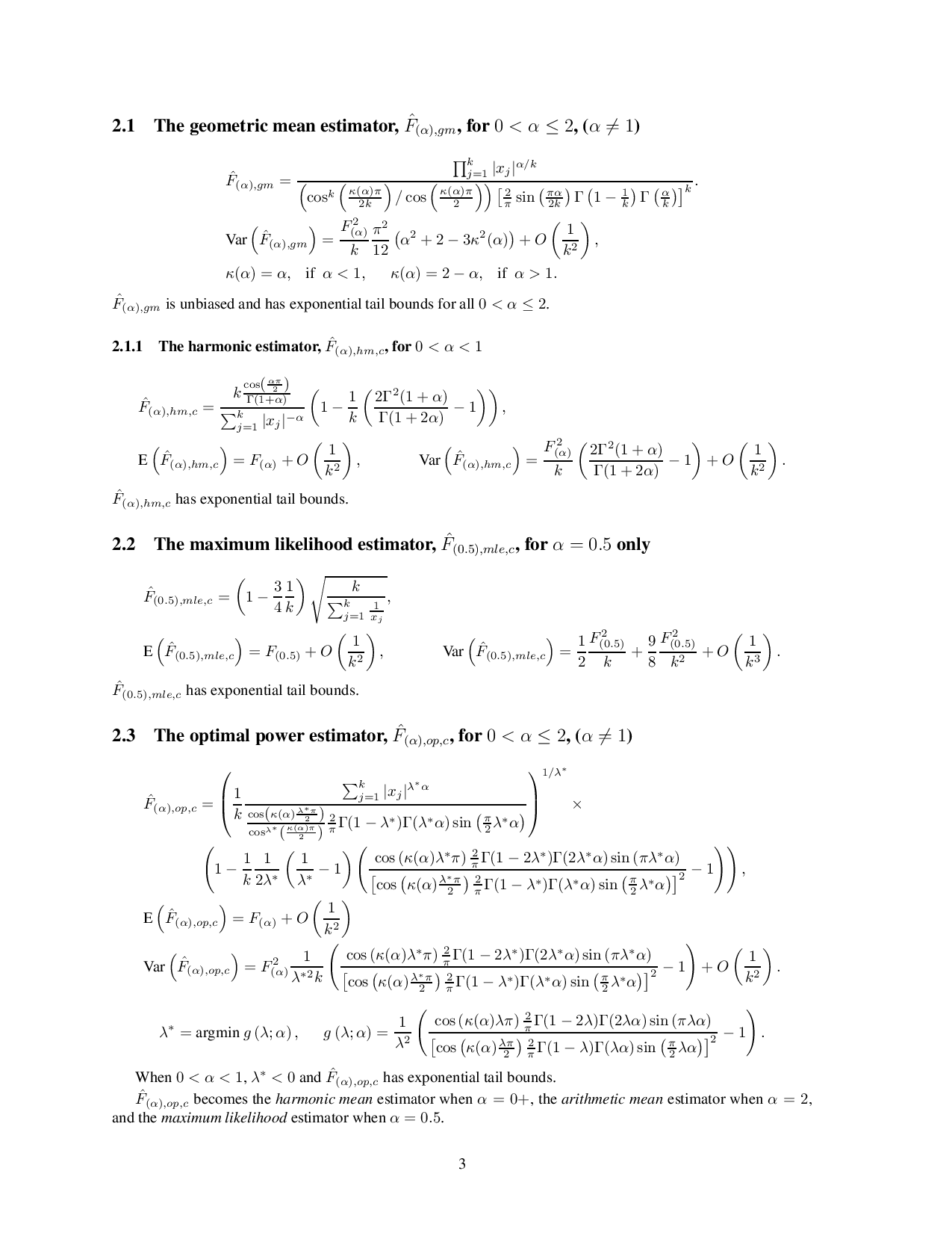
The geometric mean estimator, F(α),gm , for 0 < α ≤ 2, (α = 1)
F(α),gm is unbiased and has exponential tail bounds for all 0 < α ≤ 2.
The harmonic estimator, F(α),hm,c , for 0 < α < 1
F(α),hm,c has exponential tail bounds.
The maximum likelihood estimator, F(0.5),mle,c , for α = 0.5 only
F(0.5),mle,c has exponential tail bounds.
The optimal power estimator, F(α),op,c , for 0 < α ≤ 2, (α = 1)
When 0 < α < 1, λ * < 0 and F(α),op,c has exponential tail bounds. F(α),op,c becomes the harmonic mean estimator when α = 0+, the arithmetic mean estimator when α = 2, and the maximum likelihood estimator when α = 0.5.
Because X ∼ S α, β = 1, F (α) belongs to the location-scale family (location is zero always), one can estimate the scale parameter F (α) simply from the sample qantiles.
Assume x j ∼ S α, 1, F (α) , j = 1 to k. One possibility is to use the q-quantile of the absolute values, i.e.,
where
Denote Z = |X|, where X ∼ S α, 1, F (α) . Note that when α < 1, Z = X. Denote the probability density function of Z by f Z z; α, F (α) , the probability cumulative function by F Z z; α, F (α) , and the inverse cumulative function by
We can analyze the asymptotic (as k → ∞) variance of F(α),q , pr